SuperTrend Weighted by Divergence█ OVERVIEW
SuperTrend Weighted by Divergence is a trend-following indicator based on the classic SuperTrend, enhanced with dynamic ATR weighting driven by divergences. Its key feature is adaptive behavior: when a divergence appears, the indicator temporarily reduces the ATR multiplier, allowing the trend line to react faster to potential market reversals.
The indicator remains clean, visually clear, and well suited for traders who want to combine trend-following with early detection of weakening momentum.
█ CONCEPT
One of the biggest drawbacks of trend indicators is their lagging nature, caused by the characteristics of source data. Classic SuperTrends react only after the trend has already developed, which often leads to late entries or exits.
The idea behind SuperTrend Weighted by Divergence is to introduce dynamic adjustment of the trend line in response to the first signs of trend weakening.
Instead of treating ATR as a constant volatility buffer, the indicator temporarily modifies its impact when the market sends warning signals in the form of price–oscillator divergences.
For divergence detection, a hidden auxiliary oscillator called “MPO4 Lines – Modal Engine” (default settings) is used. This oscillator is not displayed on the chart – only the points where divergences are detected are shown as markers on price bars.
Divergences do not generate direct entry signals; they are used solely to temporarily adjust the behavior of the SuperTrend.
If, after detecting a divergence against the current trend, a divergence in line with the trend appears, the previous divergence is invalidated and the SuperTrend returns to its standard behavior (base ATR multiplier).
█ FEATURES
Data sources:
- ATR (Average True Range)
- Reference point: HL2 (high/low average)
- MPO4 Lines – Modal Engine oscillator (hidden, used only for divergence detection)
Divergence logic:
- Bullish divergence: lower low in price + higher low in the oscillator
- Bearish divergence: higher high in price + lower high in the oscillator
- Divergences are detected using pivots (left/right)
- Divergence detection is delayed by the pivot length, as confirmation requires a fixed number of bars on the right side
Divergence impact:
- After a divergence is detected, the ATR multiplier is reduced
- The reduction strength is controlled by Divergence Sensitivity
- The effect is active only for a limited number of bars – 200 bars by default (divBars)
- The effect is canceled on trend change or when a trend-aligned divergence appears
Trend change logic:
- Trend changes only after a confirmed close beyond the trailing line
- No repainting
- Trend lines break at reversal points
Visual signals:
- “Buy” and “Sell” labels only on confirmed trend changes
- Optional bar coloring based on current trend (Color bars by trend)
- Soft fill between price and the trend line
- Divergence markers (dots above/below bars) shown at the point of divergence detection, not across the entire divergence structure
Alerts:
- Buy Signal – trend change to bullish
- Sell Signal – trend change to bearish
- Bullish Divergence
- Bearish Divergence
█ HOW TO USE
Adding the indicator:
Paste the code into Pine Editor or search for “SuperTrend Weighted by Divergence” on TradingView
Main settings:
- ATR Length – ATR period
- Base ATR Multiplier – base SuperTrend width
- Pivot Length – divergence sensitivity and detection delay
- Divergence Sensitivity – strength of divergence impact (0.0–1.0)
- Color bars by trend – enable / disable bar coloring
- Line and fill colors – fully customizable
Interpretation:
- Green line and bars = uptrend
- Red line and bars = downtrend
- Divergence against the trend = possible weakening and faster SuperTrend reaction
- Trend-aligned divergence = return to standard SuperTrend behavior
- No divergence = classic, stable SuperTrend behavior
█ APPLICATIONS
Ideal for:
- Trend-following
Entering positions only in the direction of the current trend, using the SuperTrend as a directional filter.
- Early detection of trend weakness
Repeated divergences against the trend may indicate decreasing momentum and a potential upcoming reversal.
- Markets with variable dynamics (crypto, indices, forex)
Entries based on trend changes, preferably confirmed by other tools such as Fibonacci levels, RSI, support/resistance, or market structure.
- Scalping, day trading, and swing trading (with parameter adjustments)
Increasing Divergence Sensitivity to around 0.4–0.5 produces many more signals on small, often short-lived moves.
These settings work well for scalping and day trading, but are not ideal for swing trading, as they tend to generate more false signals and frequent trend changes.
█ NOTES
- Works on all markets and timeframes
- Divergences are used to adapt SuperTrend behavior, not as standalone entry signals
- Higher Divergence Sensitivity = faster reaction and more signals
- Lower Divergence Sensitivity = smoother trend and fewer changes
- Best results are achieved by tuning parameters to the instrument and trading style
Indikatoren und Strategien

Apex Trend & Liquidity Master V2.1The Apex Trend & Liquidity Master is a hybrid trading system designed to align traders with the dominant market trend while identifying key structural price levels. Unlike simple moving average crossovers or standalone support/resistance tools, this script integrates a volatility-adaptive "Trend Cloud" with a "Smart Liquidity" engine.
This integration allows the script to offer unique filtering capabilities, such as hiding counter-trend liquidity zones to reduce chart noise and focus on high-probability continuations.
How It Works
Adaptive Trend Cloud The backbone of the system is the Trend Cloud, calculated using a Hull Moving Average (HMA) base with ATR bands. The cloud expands and contracts based on market volatility.
Green Cloud: Bullish Regime. The market is trending up; look for long opportunities.
Red Cloud: Bearish Regime. The market is trending down; look for short opportunities.
Smart Liquidity Zones (with Integration) The script automatically detects Pivot Highs and Lows to draw Supply (Resistance) and Demand (Support) zones. These zones persist until price breaks through them (mitigation).
Integration Feature: A "Filter Zones by Trend" option is included in the settings. When enabled, this feature connects the Trend Cloud to the Liquidity Engine:
It will only display Demand zones when the Trend Cloud is Bullish.
It will only display Supply zones when the Trend Cloud is Bearish.
Note on Lag: Zones are based on pivots (default lookback: 10). A zone appears on the chart 10 bars after the pivot forms. These are historical structural levels.
Signal Filters Buy and Sell labels are generated when the Trend Cloud changes color, but they are filtered to ensure quality:
Volume Filter: Signals only appear if the current volume is higher than the 20-period average.
RSI Filter: Prevents buying when RSI is overbought (>70) or selling when oversold (<30).
Live HUD An on-chart dashboard provides real-time data on:
Trend Bias: Direction of the cloud.
Momentum: RSI strength (Weak/Neutral/Strong).
Volume: High vs. Low activity.
Usage Guide
Identify the Trend: Use the background fill color to determine if you should be looking for longs (Green) or shorts (Red).
Wait for Structure: Look for price to pull back into a "Smart Liquidity" zone. For example, in a Green Trend, wait for price to touch a Green Demand box.
Confirm with Momentum: Check the Dashboard. Ideally, you want to see "Strong" momentum aligning with your trade direction.
Settings: If the chart is too cluttered, enable "Filter Zones by Trend" in the settings menu to hide counter-trend boxes.
Credits & Attribution This script combines original integration logic with adapted open-source concepts:
Smart Liquidity Logic: The method for generating Supply/Demand boxes via Pivot Highs/Lows and array management is adapted from open-source logic commonly used in Smart Money Concepts (SMC) indicators, notably popularized by LuxAlgo and the broader Pine community.
Trend Logic: The volatility cloud utilizes standard Hull Moving Average (HMA) and ATR formulas.
Disclaimer This indicator is provided for educational and informational purposes only. It does not constitute financial advice. Past performance of pivot levels or trend signals does not guarantee future results.

pD Zones [MMT]pD Zones plots a clean set of intraday high‑of‑day (HOD) and low‑of‑day (LOD) zones that automatically extend forward, flip color on mitigation, and archive as historical levels for context. It is designed to give intraday traders a simple visual map of premium/discount zones derived from a chosen calculation timeframe.
Overview
Objective : Highlight the current day’s HOD/LOD wick zones as actionable intraday support and resistance.
Core logic runs on a user‑selectable source timeframe (default 15m), then projects those zones onto any chart you are trading.
Zones extend into the future, react to price via mitigation logic, and then optionally roll into a dimmed historical layer.
Zone logic
Each session, the script tracks the extreme high and low plus their wick limits (open/close‑based) on the source timeframe to form two intraday zones.
When a new day starts, the finalized prior‑day zones are “locked in” and the current day begins tracking a fresh HOD/LOD pair.
Only one HOD and one LOD zone are created per day, reducing clutter and keeping focus on the most relevant levels.
Mitigation & color flips
Active HOD zones behave as resistance: a decisive break above the top of the box flips it to a bullish (supportive) color profile, while a move back below can re‑flip it.
Active LOD zones behave as support: a break below the bottom of the box flips it to a bearish profile, and a sustained reclaim can re‑flip it as well.
Once mitigated and carried into a new day, zones are restyled with a softer historical color so they remain visible but unobtrusive.
Alerts
When price breaks a HOD zone to the upside, the script can trigger an alert message noting that HOD resistance has been broken and showing the exact level.
When price breaks a LOD zone to the downside, an alert notes that LOD support has been broken, again with the precise price printed.
These alerts are meant for intraday confirmation of structure shifts at key daily extremes, rather than frequent scalper signals.
Inputs & customization
- Calculation Timeframe: choose which timeframe defines the daily HOD/LOD zones (e.g., 5m, 15m, 1h), independent from the chart.
- Visual Settings: customize support/resistance fill colors and border color to integrate with existing layouts.
- Logic Settings:
Max Active Zones: cap how many live zones remain on the chart at once to control noise.
Max Historical Zones: keep only the most recent historical levels or show all past days.
Zone Extension Offset (Bars): control how aggressively boxes project into the future.
- Mitigation Settings: choose the historical zone color to distinguish active levels from archived ones at a glance.

QuantCrawler 5m ORB Pro - Opening Range with Confluence FiltersThis indicator captures the 5-minute Opening Range and generates entry signals using a breakout-then-retest methodology. It includes optional confluence filters to refine entries and reduce false signals.
HOW IT WORKS
1. Captures the 5-minute Opening Range (high, low, midpoint) at your selected session open
2. Waits for price to break beyond OR high or low by your defined distance
3. After breakout, monitors for price to retest the OR midpoint
4. Signals LONG after bullish breakout + midpoint retest
5. Signals SHORT after bearish breakout + midpoint retest
6. Marks invalidated signals with (X) if price breaks through the opposite side
PRE-CONFIGURED SESSIONS
- NYSE - 9:30-9:35 ET
- CME - 8:30-8:35 CT
- London - 3:00-3:05 ET
- Asia - 7:00-7:05 PM ET
- Custom - Define your own session times and timezone
BREAKOUT DISTANCE OPTIONS
Choose between fixed points or percentage-based breakout threshold. Percentage mode automatically scales to the instrument price.
CONFLUENCE FILTERS
Optional filters to add confirmation before signals fire:
- VWAP - Long requires price above VWAP, short requires below
- EMA Slope - Confirms trend direction using 20-period EMA
- Volume - Requires relative volume above 1.5x average
- FVG - Requires a Fair Value Gap supporting trade direction
- ATR - Filters Opening Ranges that are abnormally small or large relative to ATR
When filters block a valid setup, the indicator displays a BLOCKED label so you can see what you missed and why.
STATUS BOX
Real-time display showing:
- Current trade state (Building OR, Watching, Awaiting Retest, Long/Short Active)
- OR High, Low, and Midpoint levels
- Active filters and block reasons
ALERTS
Built-in alerts for Long Entry, Short Entry, or Any Entry.

Antigravity OCC Strategy (MA 5 + Delayed TSL)# OCC Strategy Optimized (MA 5 + Delayed TSL) - User Guide
## Introduction
The **OCC Strategy Optimized** is an enhanced version of the classic **Open Close Cross (OCC)** strategy. This strategy is designed for high-precision trend following, utilizing the crossover logic of Open and Close moving averages to identify market shifts. This optimized version incorporates advanced risk management, multi-timeframe analysis, and a variety of moving average types to provide a robust trading solution for modern markets.
>
> **Special Thanks:** This strategy is based on the original work of **JustUncleL**, a renowned Pine Script developer. You can find their work and profile on TradingView here: (in.tradingview.com).
---
## Key Features
### 1. Optimized Core Logic
- **MA Period (Default: 5):** The strategy is tuned with a shorter MA length to reduce lag and capture trends earlier.
- **Crossing Logic:** Signals are generated when the Moving Average of the **Close** crosses the Moving Average of the **Open**.
### 2. Multi-Timeframe (MTF) Analysis
- **Alternate Resolution:** Use a higher timeframe (Resolution Multiplier) to filter out noise. By default, it uses $3 \times$ your current chart timeframe to confirm the trend.
- **Non-Repainting:** Includes an optional delay offset to ensure signals are confirmed and do not disappear (repaint) after the bar closes.
### 3. Advanced Risk Management
This script features a hierarchical exit system to protect your capital and lock in profits:
- **Fixed Stop Loss (Initial):** Protects against sudden market reversals immediately after entry.
- **Delayed Trailing Stop Loss (TSL):**
- **Activation Delay:** The TSL only activates after the trade reaches a specific profit threshold (e.g., 1%). This prevents being stopped out too early in the trade's development.
- **Ratchet Trail:** Once activated, the stop loss "ratchets" up/down, never moving backward, ensuring you lock in profits as the trend continues.
- **Take Profit (TP):** A fixed percentage target to exit the trade at a pre-defined profit level.
### 4. Versatility
- **12 MA Types:** Choose from SMA, EMA, DEMA, TEMA, WMA, VWMA, SMMA, HullMA, LSMA, ALMA, SSMA, and TMA.
- **Trade Direction:** Toggle between Long-only, Short-only, or Both.
- **Visuals:** Optional bar coloring to visualize the trend directly on the candlesticks.
---
## User Input Guide
### Core Settings
- **Use Alternate Resolution?:** Enable this to use the MTF logic.
- **Multiplier for Alternate Resolution:** How many charts higher the "filter" timeframe should be.
- **MA Type:** Select your preferred moving average smoothing method.
- **MA Period:** The length of the Open/Close averages.
- **Delay Open/Close MA:** Use `1` or higher to force non-repainting behavior.
### Risk Management Settings
- **Use Trailing Stop Loss?:** Enables the TSL system.
- **Trailing Stop %:** The distance the stop follows behind the price.
- **TSL Activation % (Delay):** The profit % required before the TSL starts moving.
- **Initial Fixed Stop Loss %:** Your hard stop if the trade immediately goes against you.
- **Take Profit %:** Your ultimate profit target for the trade.
---
## How to Trade with This Strategy
1. **Identify the Trend:** Look for the Moving Average lines (Close vs Open) to cross.
2. **Wait for Confirmation:** If using MTF, ensure the higher timeframe also shows a trend change.
3. **Manage the Trade:** Let the TSL work. Once the trade hits the activation threshold, the TSL will take over, protecting your runner.
4. **Position Sizing:** Adjust the `Properties` tab in the script settings to match your desired capital allocation (Default is 10% of equity).
---
## Credits
Original Strategy by: **JustUncleL**
Optimized and Enhanced by: **Antigravity AI**

RSI by ErdincALGoTradeBased on the RSI logic, it only gives strong buy/sell signals when buy/sell orders occur simultaneously in 3-5-15 intervals. I'm sharing my own software to achieve 99% success for 25-30 USD movements in gold charts.

QuantCrawler ORB Break & Retest 15m - Opening Range StrategyThis indicator automates the 15-minute Opening Range Breakout and Retest strategy. It captures the high, low, and midpoint of the first 15-minute candle, then monitors for confirmed breakouts followed by midpoint retests to generate entry signals.
HOW IT WORKS
1. Captures the high, low, and midpoint of the first 15-minute candle (default 8:00-8:15 premarket)
2. Waits for price to close beyond the OR high or low by your specified breakout distance
3. After breakout confirmation, monitors for price to pull back and touch the midpoint
4. Signals LONG after bullish breakout + midpoint retest
5. Signals SHORT after bearish breakout + midpoint retest
6. Resets after each signal allowing multiple setups per session
WHY 15-MINUTE ORB
The 15-minute Opening Range captures more price action than a 5-minute OR, often providing stronger support/resistance levels. The 8:00 AM default captures premarket activity before the 9:30 open, giving you levels established before the crowd arrives.
WHY BREAKOUT + RETEST
Entering on the initial breakout often results in chop and false signals. This indicator requires confirmation - price must first prove direction by closing beyond the breakout distance, then offer a pullback entry at the midpoint. This filters out many failed breakouts.
SETTINGS
- Breakout Distance - Points beyond OR zone required to confirm breakout
- Timezone - Select your market timezone
- Opening Range Time - Customizable (default 8:00-8:15)
- Session End Time - When to stop monitoring (default 4:00 PM)
VISUAL OUTPUT
- Green line - OR High
- Red line - OR Low
- Orange dotted line - OR Midpoint
- Status box displays current state (Watching, Active, Closed)
ALERTS
Built-in alerts for Long Entry, Short Entry, or Any Entry.
Works on any timeframe chart. The indicator pulls 15-minute data automatically using request.security().

Structure Lite - Automatic Major Trend LinesStructure Lite – Pivot-Based Market Structure Visualization
OVERVIEW
Structure Lite is an open-source charting tool designed to assist traders in visualizing higher-timeframe market structure. The script identifies major swing points using high-period pivot analysis and projects structural support and resistance lines directly on the chart. Its purpose is to highlight persistent market structure while minimizing visual noise.
CORE CONCEPTS & CALCULATIONS
Pivot Identification
The script uses Pine Script’s built-in ta.pivothigh() and ta.pivotlow() functions to identify confirmed swing highs and lows. A pivot is only validated after a user-defined number of bars (Major Pivot Lookback) have formed on both sides of the price extreme, ensuring that only structurally significant pivots are selected.
Structural Pairing
Each structural line is created only after two consecutive pivots of the same type are confirmed (high-to-high or low-to-low). The script stores the price and bar index of these pivots and uses them as fixed anchor points.
Line Projection
Once a valid pivot pair is formed, the script draws a line between the two points using line.new() and extends it forward using extend.right. These lines represent projected structural boundaries rather than trade signals.
Object Management
To maintain chart clarity and performance, the script manages all drawn objects through a line array. A FIFO (First-In, First-Out) method is applied so that only the three most recent structural lines remain visible. Older lines are automatically deleted as new ones are created.
DESIGN PHILOSOPHY & ORIGINALITY
While many indicators plot frequent swing points or short-term pivots, Structure Lite focuses on structural persistence. By filtering for higher-period pivots and limiting the number of displayed projections, the script emphasizes dominant market structure rather than short-term fluctuations. This approach is intended to support discretionary analysis, not replace it.
HOW TO USE
Major Pivot Lookback
Increase the value to focus on higher-timeframe structure (e.g., swing or position trading).
Decrease the value to visualize intraday structural levels.
Visual Encoding
Green lines represent projected structural support
Red lines represent projected structural resistance
Visibility Control
A boolean input allows all structure lines to be hidden instantly to restore a clean price chart.
LIMITATIONS & DISCLAIMER
This script is a visualization tool only. It does not generate trade signals, entry or exit points, alerts, or directional forecasts. All plotted levels are derived from historical price action and may change as new pivots form. The script is provided for educational and analytical purposes and should be used in conjunction with other forms of market analysis

RSI Structure Engine (Aggressive Soft) | It measures the direction (trend) and turning points of the market via RSI(7).
But unlike the classic RSI:
It doesn't say "sell at 70 - buy at 30" ❌
Instead:
It reveals the STRUCTURE of the RSI (HH–HL / LH–LL).
That is:
Is there a trend?
Is the trend continuing?
Has the trend ended?
It divides the RSI into 3 zones:
Zone Meaning
RSI ≥ 70 Strong upward momentum (peak regime)
RSI ≤ 30 Strong downward momentum (bottom regime)
30–70 Transition / breathing space
But the key point is this 👇
The bottom/top RSI is FOLLOWED within these regimes, it doesn't lock in immediately.
What and How
🔺 🔻 Locked RSI peak/trough
HH/HL RSI upward trend
LH/LL RSI downward trend
Small points being followed (not yet locked)
If RSI HL breaks, the trend ends
WHAT YOU SHOULDN'T DO?
❌ Don't assume it's a buy-sell indicator alone
❌ Don't short just because you see RSI 70
❌ Don't long just because you see RSI 30
This indicator:
Answers the question "Which side should I be on?"
It doesn't say "Enter right here"
TREND FILTER (MAIN USE)
LONG LOOK:
Last structure: HH + HL
RSI doesn't fall below 30
🔻 HL is protected
SHORT LOOK:
Last structure: LH + LL
RSI cannot rise above 70
🔺 LH is protected
❌ Don't take a trade in the opposite direction.

SMT Divergence [Kodexius]SMT Divergence is a correlation-based divergence detector built around the Smart Money Technique concept: when two normally correlated instruments should be making similar swing progress, but one prints a new extreme while the other fails to confirm it. This “disagreement” can be a valuable contextual signal around liquidity runs, distribution phases, and potential reversal or continuation points.
The script compares the chart symbol (primary) with a user-selected comparison symbol (for example BTC vs ETH, ES vs NQ, EUR/USD vs GBP/USD) and automatically scans both instruments for confirmed swing highs and swing lows using pivot logic. Once swings are established, it checks for classic SMT conditions:
Primary makes a new swing extreme while the comparison symbol forms a non-confirming swing .
To support a wider range of markets, the indicator includes an Inverse Correlation option for pairs that typically move opposite to each other (for example DXY vs EUR/USD). With this enabled, the divergence rules are logically flipped so that the script still detects “non-confirmation” in a way that is consistent with the pair’s relationship.
The indicator is designed to be readable and actionable. It can draw divergence labels directly on the main chart, connect the relevant swing points with lines, show a compact information table with the last signal and settings, and optionally render the comparison symbol as a mini candle chart in the indicator pane for quick visual validation.
🔹 Features
🔸 Two-Symbol SMT Analysis (Primary vs Compare)
Select any comparison symbol to evaluate correlation structure and divergence. The script fetches the comparison OHLC data using the current chart timeframe to keep both series aligned for analysis.
🔸 Inverse Correlation Mode
For inversely correlated pairs, enable “Inverse Correlation” so the script interprets confirmation appropriately (for example, a higher low on the comparison instrument might be expected to correspond to a lower low on the primary, depending on the relationship). This helps avoid false conclusions when the pair naturally moves opposite.
🔸 Pivot-Based Swing with Adjustable Sensitivity
Swings are detected using confirmed pivots (left bars and right bars). This provides cleaner structural swing points compared with raw candle-to-candle comparisons, and it lets you control sensitivity for different market conditions and timeframes. The script also limits stored swing history to keep performance stable.
🔸 Flexible Detection Mode: Time Matched or Independent Swings
You can choose how swings are paired across instruments:
Time Matched searches for a comparison swing that occurred at the same pivot time as the primary swing.
Independent Swings compares each symbol’s own last two swings without requiring an exact time match.
🔸 Range Control and Noise Filtering
To reduce weak or irrelevant signals:
“Max Bars Between Swings” ensures the two swings being compared are close enough in structure to be meaningful.
“Min Price Diff (%)” can require a minimum percentage change between the primary’s last two swing prices to confirm the move is significant.
🔸 Clear Visual Output with Tooltips
When a divergence is detected, the script can print a label (“SMT”) with bullish or bearish styling and a tooltip that includes the symbol pair and the primary swing price for quick context.
🔸 Divergence Lines for Context
Optional lines connect the relevant swing points, making it easier to see the exact structure that triggered the signal. One line can be drawn on the main chart and another in the indicator pane for the comparison series.
🔸 Info Table (At a Glance)
A compact table can display the active symbols, correlation mode, total divergences stored, and the most recent signal type.
🔸 Alerts Included
Built-in alert conditions are provided for bullish SMT, bearish SMT, and any SMT event so you can automate notifications without editing the code.
🔸 Optional Comparison Candle Panel
If enabled, the indicator can plot the comparison symbol as candles in the indicator pane. This is useful for confirming whether the divergence is happening around major levels, consolidations, or impulsive legs on the secondary instrument.
🔹 Calculations
This section summarizes the core logic used by the script.
1. Data Synchronization (Comparison Symbol)
The comparison instrument is requested on the chart’s current timeframe so swing calculations are performed consistently:
=
request.security(compareSymbolInput, timeframe.period, )
This ensures pivots and swing times are derived from the same bar cadence as the primary chart.
2. Swing Detection via Confirmed Pivots
Swings are detected using pivot logic with user-defined left and right bars:
primaryPivotHigh = ta.pivothigh(high, pivotLeftBars, pivotRightBars)
primaryPivotLow = ta.pivotlow(low, pivotLeftBars, pivotRightBars)
Because pivots are confirmed only after the “right bars” have closed, the script stores each swing using an offset so the swing’s bar index and time reflect where the pivot actually occurred, not where it was confirmed.
3. Swing Storage and Retrieval
Both symbols maintain arrays of SwingPoint objects. Each new swing is pushed into the array, and older swings are dropped once the array exceeds the configured maximum. This makes the divergence engine predictable and prevents uncontrolled memory growth.
The script then retrieves the last and previous swing highs and lows (per symbol) to evaluate structure.
4. Matching Logic (Time Matched vs Independent)
When “Time Matched” is selected, the script searches the comparison swing array for a pivot that occurred at the exact same timestamp as the primary swing. When “Independent Swings” is selected, it simply uses the comparison symbol’s last two swings of the same type.
5. Bullish SMT Condition (LL vs HL)
A bullish SMT event is defined as:
Primary forms a lower low (last low < previous low)
Comparison forms a higher low (last low > previous low)
If inverse correlation is enabled, the comparison condition flips to maintain logical confirmation rules
The two primary swings must be within the configured bar distance window
Optional minimum percentage difference must be satisfied
A simple anti duplication rule prevents repeated triggers on the same structure
These checks are implemented directly in the bullish detection block.
6. Bearish SMT Condition (HH vs LH)
A bearish SMT event is defined as:
Primary forms a higher high (last high > previous high)
Comparison forms a lower high (last high < previous high)
Inverse correlation flips the comparison rule
Range checks, minimum difference filtering, and duplicate protection apply similarly
These checks are implemented in the bearish detection block.
7. Percentage Difference Filter
The optional “Min Price Diff (%)” filter measures the relative distance between the last two primary swing prices. This prevents very small structural changes from being treated as valid SMT signals.
priceDiffPerc = math.abs(lastSwing.price - prevSwing.price) / prevSwing.price * 100.0
The divergence condition is only allowed to trigger if this value exceeds the user defined threshold.
priceOk = priceDiffPerc >= minPriceDiff
This filter is especially useful on higher timeframes or during low volatility conditions, where micro structure noise can otherwise produce misleading signals.
8. Visualization and Output
When a divergence is confirmed, the script:
Stores the event in a divergence array (limited by “Max Divergences to Display”)
Draws a directional SMT label with a tooltip (optional)
Draws connecting lines using time based coordinates for clean alignment (optional)
It also updates an information table on the last bar only, and exposes alertconditions for automation workflows.

Scanner Pro MTF v9.3Manual Script Trading Scanner Pro MTF v9.3
How to Interpret Your New Tool
• Total Alignment (The Holy Grail): When you see the chart turn green (LONG) from 15m to D1, it's a high-probability signal that the cycle's bottom has been confirmed.
• Inside Bars (Yellow Dots): When they appear near a support level, they indicate indecision. If the next candle breaks upwards with high volume ('V' on the chart), it's your entry confirmation.
Here's an explanation of the symbols:
1. The Fuchsia Diamond (The "Little Squares")
This symbol represents a Squeeze (Volatility Compression).
• What it means: It appears when the Bollinger Bands move inside the Keltner Channels.
• Interpretation: It indicates that the market is in a period of extreme calm or accumulation. Historically, after a "Squeeze," an explosive price movement occurs.
• Use in your Roadmap: If Bitcoin reaches $59,000 and these fuchsia diamonds start appearing, get ready: the market is building energy for the next big surge.
2. The White "V" (Unusual Volume)
This signal appears at the top of the chart when there is a spike in volume.
• What it means: It is activated when the volume of the current candle is 50% higher than the average of the last 20 candles (volume > ta.sma(volume, 20) * 1.5).
• Interpretation: It confirms the intention. A breakout from support or resistance with a "V" is much more reliable than one without volume.
• Use in your Roadmap: If you see a strong green candle bouncing off a support level with a "V" above it, it's a sign that institutions ("Smart Money") are buying.
3. The Yellow Circle (Inside Bar)
This symbol appears above candles that are "trapped" within the range of the previous candle.
• What it means: The high of the candle is lower than the previous one, and its low is higher than the previous one.
• Interpretation: It is a sign of pause and indecision. The market is compressing the price into a narrow range.
• Strategy: Often, the price breaks out strongly after an Inside Bar. It's like a spring being compressed.
________________________________________
Trading Summary:
• Ideal Buy Signal: Price near support + Fuchsia Diamond (Squeeze) + Yellow Circle (Inside Bar) + Bullish breakout with a "V" (Volume).
• Confirmation: All of the above occurs while the chart in row D1 or H4 changes to LONG (Green).
• Ideal Sell Signal: Price near resistance + Fuchsia Diamond (Squeeze) + Yellow Circle (Inside Bar) + Bearish breakout with a "V" (Volume).
• Confirmation: All of the above occurs while the chart in row D1 or H4 changes to SHORT (Red).

Gemini Scalping Strategy [Pro Dash]Description: Gemini Scalping Strategy is a comprehensive monitoring system designed for high-frequency trading and scalping on lower timeframes (1m to 15m). This tool combines a fast-response Trailing Stop based on Average True Range (ATR) with a professional, real-time multi-factor Dashboard to provide a complete view of market structure and momentum.
Key Features:
Reactive ATR Trailing Stop: Provides immediate Buy/Sell signals based on volatility expansion and price breakouts. The trail line dynamically changes color to reflect volatility health.
Contextual Dashboard:
Choppiness Index (Corrected): Identifies whether the market is in a Trending phase (below 38.2) or a Sideways phase (above 61.8), helping to avoid "noise" in flat markets.
RSI Control Logic: Uses the 50-level pivot to define market control (Bull Control vs. Bear Control) instead of simple overbought/oversold levels.
ADX Strength: Measures trend intensity to filter out weak breakouts.
ATR Expansion: Monitors whether current volatility is above its average to confirm entry momentum.
How to use:
Entry: Primary signals are generated by the ATR triangles.
Confirmation: Use the Dashboard to verify market quality. High-probability trades occur when ATR signals align with "TREND" status on the CHOP and "BULL/BEAR CONTROL" on the RSI.
Customization: All dashboard elements (position, size, transparency, and theme) are fully customizable via the settings menu.
Disclaimer: This indicator is for educational and analytical purposes only. Trading involves significant risk, and past performance is not indicative of future results.

SMC Structure & Expectation [WavesUnchained]SMC Structure & Expectation - Professional Context & Confirmation Tool
A sophisticated Smart Money Concepts indicator that combines objective market structure analysis with intelligent expectation logic and professional order block validation. Built for traders who value context over signal spam.
4-LAYER ARCHITECTURE
Layer 1: Market Structure
✓ Objective HH/HL/LH/LL detection based on confirmed pivot swings
✓ Internal structure tracking (micro swings within major legs)
✓ Structure alignment detection (Internal + External agreement)
✓ No predictions - pure price action description
Layer 2: Expectation/Bias
✓ Logical hypotheses derived from current structure
✓ "Expect HL" in bullish structure / "Expect LH" in bearish structure
✓ "Expect Continuation" after BOS events
✓ Expectation ≠ Signal (can be wrong, that's the point)
Layer 3: Confirmation (BOS + Order Blocks)
✓ Break of Structure (BOS) detection with 2 modes:
• Conservative: Close-cross (default)
• Aggressive: High/Low-cross with optional close confirmation
✓ Professional Order Block System with 8 intelligent filters
✓ Only creates OBs when expectation is met
✓ Maximum 1 OB per direction (quality over quantity)
Layer 4: Optional Warnings
✓ Trendline break detection
✓ Early Top/Bottom warnings (volume + volatility divergence)
✓ Can be disabled for clean chart focus
PROFESSIONAL ORDER BLOCK SYSTEM
8 Quality Filters (Cascade Logic):
1. BOS-Only Guard : No OB without confirmed Break of Structure
2. Displacement Filter : Minimum 1.0 ATR momentum (customizable)
3. Location Filter : Must be in Premium (bearish) or Discount (bullish) zone
4. Size Filter : 3 modes available:
• Hard Limit: Reject oversized OBs (strict)
• Score Penalty: Allow but reduce priority (balanced, default)
• Disabled: No size filtering (permissive)
5. Volume Filter : Optional relative volume threshold
6. FVG Filter : Optional Fair Value Gap requirement
7. Mitigation Tracking : 30% penetration = mitigated (score penalty)
8. TTL (Time-To-Live) : Auto-delete after 80 bars (prevents chart clutter)
Priority Scoring System (0-100):
• HIGH Priority (>80) : Bright colors, zero transparency
• MED Priority (50-80) : Normal colors, 30% transparency
• LOW Priority (<50) : Faded colors, 60% transparency
Score Components:
✓ Displacement strength (10-30 points)
✓ FVG confluence (+20 points)
✓ Relative volume (+5-15 points)
✓ Premium/Discount location (+10-20 points)
✓ Structure alignment (+30 points if aligned, -15 if conflict)
✓ Leg strength (+15-25 points for strong impulse vs correction ratio)
✓ Size penalty (-0 to -30 points if oversized, Score Penalty mode only)
BAR COLORING MODES
Choose your preferred visual feedback:
1. Off : No bar coloring
2. Structure : Bullish/Bearish/Neutral structure states
3. Expectation : Continuation zones (green = expect bullish, red = expect bearish)
4. BOS + OB Priority (Default):
• Highlights active Order Blocks by priority
• BOS events in bright neon
• Faded structure colors when no OB active
5. Multi-Layer : Combines structure + priority intensity
6. Alignment : Shows Internal/External structure alignment (orange = conflict warning)
INTELLIGENT LOGGING SYSTEM
Priority-based log filtering to reduce noise:
• All : Every event (debug mode)
• MED+ : Only medium and high priority events
• HIGH Only : Only high priority setups
• Smart (Default): Adaptive filtering based on priority + context
Logs include:
✓ Structure changes (HH/HL/LH/LL)
✓ Expectation updates
✓ BOS events with confirmation status
✓ OB creation with full scoring breakdown
✓ OB reactions (Tap/Deep/Failure classification)
✓ Rejection reasons with "Potential Lost" analysis
CONFIGURATION HIGHLIGHTS
Layer 1: Structure
• Pivot detection length: 5 (left) / 5 (right)
• Internal structure: Optional micro-swing tracking
• Swing confirmation: Closes beyond pivot required
Layer 2: Expectation
• Expectation expiry: 40 bars (auto-reset after timeout)
• Visual feedback: Labels + optional expectation zones
Layer 3: Confirmation
• BOS Mode: Close-cross (conservative) / High/Low-cross (aggressive)
• Close Confirmation: Optional 3-bar window for aggro mode
• Displacement: Min 1.0 ATR (customizable)
• Size Filter Mode: Hard Limit / Score Penalty / Disabled
• OB Location: 38% discount / 62% premium thresholds
• OB Size Range: 0.3-1.2 ATR (customizable)
• TTL: 80 bars default
• Volume Filter: Optional, 1.0x minimum
• FVG Requirement: Optional
Layer 4: Warnings
• Trendline break detection
• Early Top/Bottom signals
• Can be fully disabled
BEST USE CASES
✓ Context Tool : Understand where you are in the market cycle
✓ Confirmation Filter : Validate trade ideas with structure alignment
✓ Order Block Trading : High-probability zones with priority scoring
✓ Educational : Learn SMC concepts with transparent logic
✓ Multi-Timeframe Analysis : Combine with HTF structure for confluence
Optimized for:
• Commodities (NatGas, Gold, Oil)
• 1H - 4H timeframes
• Swing trading / Intraday positioning
KEY FEATURES SUMMARY
✓ Zero signal spam - only high-conviction setups
✓ Transparent scoring system - know why each OB matters
✓ Adaptive to market conditions - structure alignment detection
✓ Flexible filtering - customize to your risk tolerance
✓ Priority-based visuals - instantly identify best opportunities
✓ Professional logging - learn from rejections and acceptances
✓ Clean chart - auto-cleanup with TTL system
✓ Bar coloring modes - choose your visual feedback style
✓ Size Filter Mode - prevent blocking of high-quality oversized setups
PHILOSOPHY
This indicator follows the principle: "Context over signals, quality over quantity"
Expectations can be wrong - that's the point. They help you stay aware of the most likely scenario while remaining open to structure changes. When expectation is met AND confirmed by BOS + quality OB, you get a high-conviction setup.
Not a holy grail. Not a signal service. A professional analysis tool.
Version: 1.0.0
Author: WavesUnchained
Pine Script: v6

Gann ArchitectThe Gann Architect is a quantitative geometric engine designed to solve the primary limitation of standard Gann tools: Scaling.
Standard Gann Fans use fixed angles (e.g., 45 degrees for 1:1), which often fail when applied to volatile assets or different timeframes because they do not account for the specific price-to-time ratio of the asset. This indicator solves this by calculating a Dynamic Slope. It identifies the initial "Impulse Phase" (Anchor Low → First Major High) and mathematically "squares" the chart to fit that specific market structure.
Key Features
Dynamic Squaring: Automatically calculates the true 1:1 Master Line based on the asset's actual volatility, not an arbitrary angle.
Quantitative Alerts: Includes a built-in alert system. You can set alerts for "Crossed 1:1" (Trend Break), "Structural Fail 1:2" (Support Break), or "Impulse Breakout 2:1".
Real-Time Data Panel: A dashboard displays the exact price targets for the geometric levels, removing the need to eyeball the lines.
Efficiency: Uses a circular buffer memory system to ensure high performance ("100% potential") without slowing down your chart.
How to Use
This tool is designed as a Trend Following & Structure Map, not a reversal signal.
The 1:1 Line (Solid): This represents the "True Trend." In a strong bullish phase, price should respect this line as dynamic support. A confirmed close below this line often signals momentum loss.
The 1:2 Line (Bottom Support): This acts as the "Structural Floor." If price loses the 1:1 but holds the 1:2, it is considered a healthy correction. A break below the 1:2 typically invalidates the geometric structure of the current cycle.
The 2:1 Line (Top Resistance): This marks the "Impulse Zone." A break above this line suggests parabolic or over-extended behaviour.
Settings
Cycle Stiffness: Controls the sensitivity of the pivot detection. Increase this value (e.g., to 4 or 5) to filter out noise and focus on macro trends.
Anchor Pivot #: Allows you to select which historical cycle bottom to anchor the geometry to (1 = most recent confirmed bottom).
Slope Multiplier: Adjusts the aggressiveness of the fan. Default is 1.0 (Geometric Standard).
Technical Disclosure (Repainting & Lag)
This script utilises a Confirmed Pivot Detection system.
Signal Lag: To ensure reliability, the geometric fans anchor to confirmed pivots. A pivot is only confirmed after Right Length bars have passed. Therefore, the fans will appear on the chart with a slight delay relative to the absolute low.
Repainting: Once a pivot is confirmed and the fans are drawn, the lines for that specific cycle do not repaint history. However, if a new, lower low forms that invalidates the previous structure, the script will dynamically shift to the new anchor point to maintain geometric accuracy.
Disclaimer This script is for educational and experimental purposes only. Geometric analysis is a mapping tool, not a guarantee of future price action. Always use proper risk management. Past performance of geometric levels does not guarantee future results.

Trend Pulse Channel StrategyOverview
Trend Pulse Channel Strategy is a long-only trend-following breakout strategy built around an adaptive multi-pole smoothing filter and a volatility-adjusted price channel.
The strategy is designed to participate in sustained directional moves by entering only when price confirms momentum strength beyond a dynamic upper boundary, while avoiding mean-reversion and low-quality consolidation phases.
This script is published as a strategy and includes realistic backtesting assumptions for position sizing, commissions, and slippage.
Core Concept
At the heart of the strategy is a multi-pole adaptive EMA-based filter, inspired by advanced digital signal smoothing techniques.
Using multiple poles allows the filter to reduce noise while preserving responsiveness to genuine trend changes.
To adapt the channel width to changing market conditions, the strategy applies the same filtering logic to True Range, producing a volatility-aware envelope rather than a static or fixed-percentage band.
This combination allows the strategy to:
Track directional bias using a smoothed central filter
Adjust channel width dynamically based on market volatility
Trigger entries only when price expansion confirms trend strength
Entry Logic
A long position is opened when:
Price crosses above the upper channel band
The signal occurs within the user-defined date range
This condition represents a volatility-confirmed breakout aligned with the prevailing directional filter.
Exit Logic
The long position is closed when:
Price crosses back below the upper band
This exit logic aims to stay in trending moves while exiting when upside momentum weakens.
The strategy does not open short positions by design.
Inputs and Defaults
The default inputs are selected to balance smoothness, responsiveness, and stability:
Source (HLC3): Reduces single-price noise by averaging high, low, and close
Period (144): Defines the primary smoothing horizon of the adaptive filter
Poles (4): Controls the smoothness vs. responsiveness trade-off
Range Multiplier (1.414): Scales the volatility envelope using filtered True Range
Reduced Lag (optional): Applies lag compensation to improve responsiveness
Fast Response (optional): Blends multi-pole and single-pole filters for quicker reaction at the cost of smoothness
All inputs are fully configurable and can be adjusted to suit different instruments and timeframes.
Risk Management & Position Sizing
The strategy uses:
Position size: 10% of equity per trade
No pyramiding
Long positions only
This sizing approach is intended to reflect sustainable risk exposure rather than aggressive capital deployment. Users may further adjust position size based on their own risk tolerance.
Backtesting Assumptions
The strategy is tested using :
Initial capital: 10,000
Commission: 0.1%
Slippage: 1 tick
Order fill model: Standard OHLC
These settings are chosen to provide more realistic performance estimates compared to idealized backtests.
This strategy is best suited for :
Trend-oriented markets
Higher timeframes where breakouts are more reliable
Users seeking systematic trend participation rather than frequent scalping
In sideways or range-bound market conditions, price may cross the channel boundaries frequently.
This can result in a higher number of entry and exit signals that do not develop into sustained trends.
For this reason, the strategy should be used with an understanding of basic technical analysis concepts, including market structure, trend identification, and consolidation behavior.
It is intended as a decision-support tool, not a standalone trading system.
Users—whether beginners or experienced traders—should avoid relying solely on this strategy and are encouraged to combine it with broader market context and additional analysis methods.
Disclaimer
This script is provided for educational and analytical purposes only. It does not constitute financial advice. Past performance does not guarantee future results.
Support and ResistanceSupport & Resistance Zones
This indicator automatically identifies support and resistance zones by clustering confirmed pivot highs and lows into statistically valid price areas.
Instead of drawing single horizontal lines, it creates price zones whose width is dynamically controlled using ATR (Average True Range), allowing the zones to adapt to market volatility.
Core Logic
The indicator scans a user-defined number of historical bars and detects pivot highs and pivot lows using a configurable pivot strength.
Each new pivot is evaluated against previously detected zones:
A zone becomes visible only after receiving sufficient confirmation (minimum number of pivot touches).
This ensures that only structurally meaningful levels are drawn.
Zone Construction Rules
Zones are formed by grouping pivot points whose total price range remains within ATR range
Each zone expands dynamically as new pivots confirm it
Zones are drawn as rectangular areas, not lines
Zones extend to the right, remaining active until price structure changes
This approach avoids over-plotting and reduces noise commonly seen in traditional support/resistance tools.
Dynamic Zone Coloring
Zones automatically change color based on current price position:
Support Color → Price is above the zone
Resistance Color → Price is below the zone
Neutral (In-Zone) Color → Price is trading inside the zone
This makes it easy to visually assess market context without additional indicators.
Inputs Explained
Logic Settings
Bars to Apply
Number of historical bars scanned to detect pivots and construct zones.
Pivot Strength
Number of candles required on both sides of a pivot high/low for confirmation.
Min Pivot Confirmation
Minimum number of aligned pivots required before a zone is drawn.
Styling
Support, resistance, and in-zone colors
Zone fill transparency
Why This Approach
Uses price structure, not arbitrary levels
Adapts to market volatility via ATR
Filters out weak, single-touch levels
Works across all markets and timeframes
This indicator is designed to highlight areas of interest, not generate buy or sell signals.
It is best used in combination with trend, momentum, or volume-based tools.

Open Interest Bubbles [BackQuant]Open Interest Bubbles
A visual OI positioning overlay that aggregates futures open interest across major venues, normalizes it into a consistent “signal strength” scale, then plots extreme events as bubbles, labels, and optional horizontal levels directly on price.
What this is for
Open interest is one of the cleanest ways to track when positioning is building, unwinding, or aggressively shifting. The problem is raw OI is noisy, exchange-specific, and hard to compare across time. This script solves that by:
- Aggregating OI across multiple exchanges.
- Letting you choose what “OI signal” you care about (raw, delta, percent versions).
- Normalizing the signal so “big events” are easy to spot.
- Plotting those events as bubbles and levels at the exact price they occurred.
You end up with a clean, fast visual map of where large positioning changes occurred, and where those events may later matter as reaction points.
────────────────────────────────────────────────────────────
Plotting types (what you can display)
Bubbles
This mode plots OI events as size-bucketed circles on the chart. Bigger bubbles represent stronger normalized events. You can tune:
- Bubble sizing by bucket (Tiny → Huge).
- Heatmap vs solid color styling.
- Signed vs unsigned coloring (positive/negative separation or magnitude-only).
Best use:
- Spotting “where something changed” at a glance.
- Identifying clusters of positioning events around key price zones.
- Seeing whether the market is repeatedly building/closing positions at similar levels.
Levels
Levels mode draws a horizontal line at the anchor price when an extreme OI event triggers. These act like “positioning memory” levels:
- They do not claim to be support/resistance by themselves.
- They highlight prices where the derivatives market clearly did something meaningful.
Best use:
- Marking potential reaction zones.
- Combining with your price action tools (structure, OBs, FVGs) to confirm whether an OI level aligns with a technical level.
- Building a “map” of where leverage likely entered or exited.
Modes available in the script:
- Off
- Bubbles
- Bubbles + Labels
- Labels Only
- Levels + Labels
────────────────────────────────────────────────────────────
Aggregated Open Interest source (multi-exchange)
This indicator builds a single aggregated OI series by requesting OI data from multiple exchanges and summing it. You can toggle exchanges on/off:
- Binance, Bybit, OKX, Bitget, Kraken, HTX, Deribit
You can also choose OI units:
- COIN , OI in base units (native sizing)
- USD , converted for a dollar-value representation
Important note:
Not every symbol has OI data on every venue. If the script cannot build an aggregated series for the symbol, it will throw an error rather than quietly plotting garbage.
────────────────────────────────────────────────────────────
OI Source, what the bubbles are measuring
You control what “signal” is normalized and plotted:
- Delta , change in aggregated OI from the prior bar.
Use when you want to highlight bursts of new positioning or sudden unwind events.
- Raw OI , the aggregated open interest level itself.
Use when you want to highlight absolute positioning build-up periods.
- Delta % , percent change in OI.
Use when you want moves normalized to the current OI regime, useful across different market eras.
- Raw OI % , percent change form of the raw series.
Use when you want relative changes rather than absolute size.
Practical guidance:
- Delta modes are best for “event detection”.
- Raw modes are better for “regime context” and whether positioning is structurally rising or fading.
────────────────────────────────────────────────────────────
Normalization (the key to making it readable)
Because OI varies massively across assets and time, the script includes multiple normalization modes to convert your chosen OI source into a comparable “strength” value.
Options:
- ZScore , deviation from a rolling mean in standard deviation units.
- StdNorm , scaled by rolling standard deviation.
- AbsZScore , absolute value version for magnitude-only mapping.
- AbsStdNorm , absolute value version for magnitude-only mapping.
- None , plots raw values (advanced users only, often too noisy visually).
Why this matters:
Normalization makes a “1.5” or “3.0” threshold mean something across different assets and timeframes, instead of being stuck to raw OI units.
────────────────────────────────────────────────────────────
Threshold system (when bubbles/levels trigger)
The plot is driven by two user thresholds:
- Base Threshold
Controls where “meaningful” events start. Raising this reduces noise and focuses on larger deviations.
- Extreme Threshold
Controls what qualifies as a top-tier event. Extreme events are what you typically want to convert into labels and levels.
You also control side filtering:
- Both , show positive and negative events.
- Positive Only , show only increases (or positive signal side depending on source).
- Negative Only , show only decreases (or negative signal side).
In practice:
- Use Base Threshold to tune chart cleanliness.
- Use Extreme Threshold to mark only the “big stuff” that tends to matter later.
────────────────────────────────────────────────────────────
Anchor Source (where the bubble/level is placed)
The indicator places bubbles, labels, and levels at a price anchor you choose:
- HL2, Close, Open, High, Low, VWAP
This is important because “where you pin the event” changes how it reads:
- Close is clean and consistent for backtesting and candle-close logic.
- High/Low can better represent where the fight occurred intrabar.
- VWAP can be useful for “fair price” anchoring in active markets.
────────────────────────────────────────────────────────────
Style system (theme, palette, signed logic)
This script is built to look good and stay readable on busy charts.
Themes
- BackQuant, Classic, Ice, Fire, Mono, Custom
Palette Mode
- Solid , one consistent color
- Heatmap , intensity increases with magnitude
- Single Color Adaptive , adapts to chart background for clarity
Side Coloring
- Signed , positive and negative events can use different ramps
- Unsigned , magnitude-only coloring
Negative theme handling:
- Auto (mirrors your chosen theme),
- Invert (flips the ramp),
- Custom (fully user-defined negative palette).
What this gives you:
- You can run a clean “mono” look for professional charts.
- Or a high-contrast heatmap for fast scanning.
- Or fully custom branding colors for BackQuant-style presentation.
────────────────────────────────────────────────────────────
Labels (what’s inside the label)
When labels are enabled, the script can display:
- OI , the aggregated OI value
- OI + Norm , OI plus normalized strength
- Norm Only , just the normalized strength
- Src + Norm , the selected source value (Delta, Raw, %) plus normalized strength
You can also control:
- Left/Center/Right label alignment
- Number formatting style (Raw, Compact, Volume format)
Best practice:
- Use “Src + Norm” when you want both the raw event size and its rarity.
- Use “Norm Only” when you want a clean, minimal chart.
────────────────────────────────────────────────────────────
Levels and object limits (performance and cleanliness)
Because this script draws objects, it includes a hard cleanup system:
- You set Max Levels / Labels to control chart clutter.
- The script deletes older lines/labels when the limit is exceeded.
This is critical if you trade lower timeframes, where OI events can trigger frequently.
────────────────────────────────────────────────────────────
How to interpret the signals
What a large bubble usually means:
- A statistically large positioning change relative to recent history.
- This can represent fresh leverage entering, forced liquidations, or aggressive de-risking, depending on direction and context.
How to use levels:
- Treat them as “attention levels”, not automatic entries.
- Combine them with structure and liquidity tools:
- If price revisits an OI level and shows rejection, it often confirms that level mattered.
- If price slices through with no reaction, it often indicates the OI event was transitional, not defended.
Common setups:
- Clustered extreme bubbles near a breakout zone, then retest later.
- Extreme negative event at capitulation low, followed by structure flip.
- Extreme positive build into resistance, then unwind and mean reversion.
Also, please check out @NoveltyTrade for the OI Aggregation logic & pulling the data source!
Here is the original script:

Statistcal Daily Profile & Ranges# Statistical Daily Profile & Ranges - TradingView Publication Guide
## Overview
The **Statistical Daily Profile & Ranges** indicator is a comprehensive tool designed to analyze intraday session behavior and daily range characteristics. It combines Average Daily Range (ADR) projection levels with detailed session-by-session statistics and probability-based trading insights derived from historical price action patterns.
## What This Indicator Does
This indicator provides traders with three core analytical components:
1. **ADR Projection Levels** - Dynamic support/resistance levels based on historical daily ranges
2. **Session Range Analysis** - Visual boxes and statistical breakdowns for four key trading sessions
3. **Dynamic Probability Display** - Real-time probability statistics based on overnight session relationships
## How It Works
### Average Daily Range (ADR) Calculation
The indicator calculates the average daily range over a user-defined lookback period (default: 10 days) and projects this range from each day's opening price. This creates two key levels:
- **ADR High**: Opening price + average daily range
- **ADR Low**: Opening price - average daily range
- **ADR Median**: The opening price (middle of the projected range)
These levels are recalculated at the start of each trading day and extend forward, providing dynamic support and resistance zones based on recent volatility characteristics.
### Session Tracking & Statistics
The indicator monitors four distinct trading sessions (times in Eastern Time):
1. **Asia Session** (8:00 PM - 2:00 AM)
2. **London Session** (2:00 AM - 8:00 AM)
3. **NY Open** (8:00 AM - 9:00 AM)
4. **NY Initial Balance** (9:30 AM - 10:30 AM)
For each session, the indicator:
- Draws a colored box showing the session's high-to-low range
- Tracks the opening price, high, and low
- Stores historical data for statistical analysis
- Calculates average ranges by day of week (Monday through Friday)
The session statistics are displayed in a customizable table showing average point ranges for each session across different weekdays, helping traders identify which sessions and days typically produce the most movement.
### Dynamic Probability System
The indicator analyzes the relationship between the Asia and London sessions to determine the current market setup. After the London session closes, it automatically detects one of four possible conditions:
**1. London Engulfs Asia**
- London session breaks both above Asia's high AND below Asia's low
- This indicates strong momentum during the European session
- Most common occurrence pattern
**2. Asia Engulfs London**
- Asia session range completely contains the London session range
- Indicates consolidation during London hours
- Relatively rare pattern (occurs approximately 5.36% of the time)
**3. London Partially Engulfs Upwards**
- London breaks above Asia's high but stays above Asia's low
- Suggests bullish momentum continuation from Asia into London
**4. London Partially Engulfs Downwards**
- London breaks below Asia's low but stays below Asia's high
- Suggests bearish momentum continuation from Asia into London
Once a condition is detected, the indicator displays a probability table showing historically observed outcomes for that specific setup, including:
- Probability of NY session taking out key levels (Asia high/low, London high/low)
- Probability of NY session engulfing the entire overnight range
- Directional bias for NY Cash session (9:30 AM - 4:00 PM)
## How to Use This Indicator
### Initial Setup
1. Add the indicator to your chart (works on any intraday timeframe below Daily)
2. Adjust the **ADR Days** setting (default: 10) to control the lookback period for range calculation
3. Adjust the **Session Lookback Days** setting (default: 50) to determine how much historical data feeds the statistics tables
### Reading the ADR Levels
- Use the **ADR High** and **ADR Low** lines as potential profit targets or areas where price may encounter resistance
- The **ADR Median** line represents the opening price and can act as a pivot point for intraday directional bias
- If price reaches the ADR High early in the session, it suggests strong bullish momentum; conversely for ADR Low
- These levels adapt daily based on recent volatility, making them more responsive than static levels
### Interpreting Session Boxes
- **Session boxes** visually highlight when each trading session is active and its price range
- Larger boxes indicate higher volatility during that session
- Compare current session ranges to the statistical averages shown in the table
- Sessions that are unusually quiet or active relative to historical averages may signal compression or expansion
### Using the Session Statistics Table
- The table shows average point ranges for each session broken down by weekday
- Identify which sessions typically produce the most movement on specific days
- For example, if London on Thursdays averages 40 points while Mondays average 25 points, you can adjust position sizing or expectations accordingly
- The **Total** column shows the overall average across all days
- Sample sizes (shown in brackets if enabled) indicate data reliability
### Trading with the Probability Table
The probability table updates dynamically after the London session closes and shows statistically probable outcomes based on 12 years of NQ futures data.
**Important Limitations:**
- **These probabilities are derived from NQ (Nasdaq E-mini futures) data only**
- **Do NOT apply these probability statistics to other instruments** (ES, stocks, forex, etc.)
- The probabilities represent historical frequencies, not guarantees
- Always combine with your own analysis, risk management, and market context
**How to Apply the Probabilities:**
When **London Engulfs Asia**:
- Watch for NY session to take out London's extremes (72.33% probability for high, 71.12% for low)
- Slight bullish bias in NY Cash session (54.80% vs 45.20%)
- Lower probability of complete overnight engulfment (44.13%)
When **Asia Engulfs London** (rare - 5.36% occurrence):
- Higher probability NY takes Asia's high (75.86%)
- Moderately high probability NY takes Asia's low (65.52%)
- Slight increase in bullish bias (58.42% vs 41.58%)
- Recognize this as an unusual setup
When **London Partially Engulfs Upwards**:
- Very high probability NY takes London high (81.51%)
- Strong probability NY takes London low (64.45%)
- Moderate probability NY takes Asian low (53.16%)
- Slight bullish bias (55.52%)
When **London Partially Engulfs Downwards**:
- Very high probability NY takes London low (75.29%)
- Strong probability NY takes London high (68.80%)
- Moderate probability NY takes Asian high (56.44%)
- Slight bullish bias maintained (52.99%)
### Practical Trading Applications
**Scenario 1: Range Projection**
If the ADR is 500 points and the market opens at 25,000:
- ADR High: 25,500 (potential resistance/target)
- ADR Low: 24,500 (potential support/target)
- Monitor how price interacts with these levels throughout the day
**Scenario 2: Session-Based Trading**
Using the statistics table, you notice London on Wednesdays averages 35 points. During a Wednesday London session:
- If London has already moved 30 points, the session may be exhausting its typical range
- If London has only moved 15 points with an hour remaining, there may be expansion potential
- Adjust stop losses and targets based on typical session behavior
**Scenario 3: Probability-Based Setup**
It's 8:05 AM ET and the indicator shows "London Partially Engulfs Upwards":
- You now know there's an 81.51% historical probability NY will take out London's high
- There's a 53.16% probability NY will reach down to Asia's low
- The NY Cash session has a slight bullish bias (55.52%)
- Consider this alongside your technical analysis for directional bias and level targeting
## Customization Options
### Visual Settings
- **Line Width**: Adjust thickness of ADR levels
- **ADR Color/Style**: Customize appearance of ADR projection lines (solid, dashed, dotted)
- **Median Line**: Toggle visibility and customize appearance separately
- **Session Box Colors**: Customize each session's box color independently
- **Show Session Boxes**: Toggle session box visibility on/off
### Label Settings
- **ADR Labels**: Show/hide labels for ADR High and ADR Low, adjust size
- **Median Label**: Separate control for median line label
- **Session Labels**: Show/hide session name labels, adjust size
- **Label Colors**: Customize text colors for all labels
### Table Settings
- **Session Stats Table**: Position (9 locations available), size (Tiny to Huge), toggle on/off
- **Sample Sizes**: Show/hide the number of historical samples used for each calculation
- **Probabilities Table**: Separate position and size controls, toggle on/off
### Session Times
- Each session's time range can be customized to fit different markets or preferences
- All times are in Eastern Time (America/New_York timezone)
## Technical Notes
### Data Requirements
- The indicator requires sufficient historical data based on your lookback settings
- Minimum recommended: 50+ days of intraday data for reliable statistics
- Works on any timeframe below Daily (1-minute, 5-minute, 15-minute, etc.)
### Calculation Methodology
- **ADR Calculation**: Simple average of absolute daily high-low ranges
- **Session Statistics**: Mean average of ranges for each session filtered by day of week
- **Condition Detection**: Boolean logic comparing session high/low relationships
- All calculations update in real-time as new bars form
### Probability Data Source
The probability statistics displayed in the dynamic table are derived from:
- **Dataset**: 12 years of NQ (Nasdaq E-mini futures) historical data
- **Methodology**: Frequency analysis of outcomes following specific setup conditions
- **Time Period**: Multiple market cycles including various volatility regimes
**Critical Warning**: These probabilities are specific to NQ and reflect that instrument's behavior patterns. Market microstructure, participant behavior, and volatility characteristics differ significantly across instruments. Do not apply these NQ-derived probabilities to other markets (ES, RTY, YM, individual stocks, forex, commodities, etc.).
## Best Practices
1. **Combine with Other Analysis**: Use this indicator as one component of a complete trading methodology, not a standalone system
2. **Respect Risk Management**: Probabilities are not certainties; always use proper position sizing and stop losses
3. **Context Matters**: High-impact news events, holiday trading, and extreme volatility can invalidate typical patterns
4. **Verify Statistics**: Monitor your own results and compare to the displayed probabilities
5. **Adapt Session Times**: If trading instruments with different active hours, adjust session times accordingly
6. **Regular Calibration**: Periodically review if the session averages and probabilities remain relevant to current market conditions
## Understanding Originality
This indicator is original in its approach to combining three analytical frameworks into a single tool:
1. **Dynamic ADR Projection**: Unlike static pivot points, these levels adapt daily based on recent volatility
2. **Session-Specific Statistics**: Goes beyond simple volume profiles by quantifying average ranges for specific time windows across weekdays
3. **Conditional Probability Display**: Automatically detects overnight session relationships and displays relevant probability data rather than showing all scenarios simultaneously
The conditional logic system that determines which probability set to display is a key differentiator—traders only see the statistics relevant to the current market setup, reducing information overload and improving decision-making clarity.
## Summary
The **Statistical Daily Profile & Ranges** indicator provides traders with a comprehensive framework for understanding daily range potential, session-specific behavior patterns, and probability-based setup analysis. By combining ADR projection levels with detailed session statistics and dynamic probability displays, traders gain multiple perspectives on potential price movement within the trading day.
The indicator is most effective when used to:
- Set realistic profit targets based on average daily range
- Identify which sessions typically produce movement on specific weekdays
- Understand probability-weighted outcomes for different overnight setup conditions (NQ only)
- Visualize session ranges and compare them to historical averages
Remember that all statistical analysis reflects historical patterns, and market behavior can change. Always combine indicator signals with sound risk management, proper position sizing, and your own market analysis.

Mass Sentiment & Contrarian (Only Signals)
________________________________________
📘 Contrarian Mass Sentiment Indicator Manual
This indicator is designed to identify moments of psychological exhaustion in the market. Its philosophy is "buy panic and sell euphoria."
1. Where and how is the data taken from?
The indicator analyzes three real-time data sources to filter the signals:
• Psychology (RSI): We use the Relative Strength Index (RSI) to measure the speed and change in price movements.
• If the RSI is very high (>70-75), the "mass" is overbuying (greed).
• If the RSI is very low (<25-30), the "mass" is overselling (panic).
• Price Action (Candlesticks): It is not enough for the RSI to be at an extreme. The indicator looks for reversal patterns (Hammer, Shooting Star, or Engulfing candlesticks). This confirms that the price has indeed found a top or bottom.
• Price Action (Candlesticks): It is not enough for the RSI to be at an extreme. The indicator looks for reversal patterns (Hammer, Shooting Star, or Engulfing candlesticks). This confirms that the price has actually found a top or bottom.
• Price Action (Candlesticks): • Market Effort (Volume): At "Strong" levels, the indicator requires volume to exceed its 20-period moving average. This identifies a volume climax, which typically marks the end of a move.
________________________________________
2. User Manual: Signal Interpretation
The indicator classifies opportunities according to their probability of success:
A. Intensity Levels
Label Strength Meaning Suggested Action
F-VTA / F-CPA Strong Maximum euphoria/panic + Volume + Reversal candle. High probability signal. Look for immediate entry.
M-VTA / M-CPA Medium Standard overload level + Reversal candle. Solid technical confirmation. Trade in favor of the structure.
D-VTA / D-CPA Weak The RSI is just beginning to reverse from moderate levels. Early warning. Do not enter without confirmation using other tools.
B. Trade Execution (Contrarian)
1. Location: Wait for a label to appear. The best are the Strong (F) or Medium (M) lines.
2. Stop Loss: Always place it a few pips/points above the high of the signal candle (for selling) or below the low (for buying).
3. Take Profit: * Target 1: The mid-RSI level (50).
or Target 2: The opposite RSI band (if you sold at 70, aim to close at 30).
________________________________________
3. Golden Tips
• Avoid sideways markets: In very narrow ranges, the RSI can give false signals ("wobbling"). Look for signals that occur after a clear and extended trend.
• Timeframes: The indicator is most reliable on 15-minute, 1-hour, and 4-hour timeframes. On the 1-minute timeframe, market "noise" can generate constant weak signals.
• Confluence: If you see an F-VTA (Strong Sell) signal right at a historical price resistance, the probability of success increases dramatically.

Low-High Waves for NeowaveOpen your chart at daily and hide the symbol graphic. Now you can see the waves. It’s including limited data sorry for this but I’m not a programmer and TradingView have limitations.

Buy / Sell Volume Header / NPR21📊 Buy / Sell Volume Header – NPR21
Overview
Buy / Sell Volume Header – NPR21 displays real-time Buy vs Sell volume dominance in a clean, Thinkorswim-style fixed header at the top of the chart.
Instead of cluttering candles with labels, this indicator presents volume information in a compact, side-by-side header, allowing traders to instantly gauge who is in control of the current bar—buyers or sellers—without losing focus on price action.
How It Works
Buy and Sell volume are estimated using candle structure:
Buy Volume is derived from the portion of the candle closing above the low
Sell Volume is derived from the portion of the candle closing below the high
Percentages show relative dominance for the most recently confirmed bar
This approach provides a fast, intuitive order-flow bias that works across futures, indices, crypto, and equities.
Key Features
✔ Thinkorswim-style fixed header
✔ Side-by-side Buy | Sell layout (no overlap)
✔ Bold green/red backgrounds with white text
✔ Compact font for intraday trading
✔ Updates only on confirmed bars (non-repainting)
✔ No candle clutter
✔ Optimized for scalping and intraday trading
Best Use Cases
Confirming buyer vs seller control
Adding confluence to:
Momentum indicators
VWAP / EMA strategies
Market structure & BOS setups
Quick decision support during:
Breakouts
Pullbacks
Range highs/lows
This tool is designed to be confirmation, not a standalone signal.
Notes
This is a volume estimation tool, not true bid/ask or footprint data
Best used alongside price action and structure
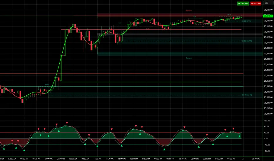
Swing Elite Trend Direction [Free]Swing Elite Trend Direction
This indicator automatically identifies and labels market structure by detecting swing highs and swing lows, then classifying them as Higher Highs (HH), Higher Lows (HL), Lower Highs (LH), and Lower Lows (LL).
🔍 What It Does
The indicator uses a depth-based pivot detection algorithm to find significant swing points in price action. Each swing is then compared to the previous swing of the same type to determine the market structure:
HH (Higher High): Current swing high is above the previous swing high → bullish structure
HL (Higher Low): Current swing low is above the previous swing low → bullish structure
LH (Lower High): Current swing high is below the previous swing high → bearish structure
LL (Lower Low): Current swing low is below the previous swing low → bearish structure
📈 How To Use
Trend Identification:
Bullish trend is confirmed when you see HH followed by HL (or HL followed by HH)
Bearish trend is confirmed when you see LL followed by LH (or LH followed by LL)
The zigzag line color changes based on confirmed trend direction
Trade Setups:
In a bullish trend, look for pullbacks to HL areas for long entries
In a bearish trend, look for rallies to LH areas for short entries
Trend changes are signaled when structure breaks (e.g., bullish trend making a LL)
Depth Setting:
Higher depth values (e.g., 34-55) capture major swings for higher timeframe analysis
Lower depth values (e.g., 8-21) capture minor swings for shorter-term trading
Adjust based on your trading style and timeframe

Elite Monday Range V3- ProfessionalElite Monday Range V3 - Advanced Institutional Bias & Analysis
Overview
The Elite Monday Range V3 is a high-performance decision-support tool designed for traders who utilize the "Weekly Open" and "Monday's Range" as their primary benchmark for the trading week. Unlike standard range indicators, this script employs an advanced Multi-Asset Analysis Engine to determine the weekly bias with institutional-grade precision.
It doesn't just draw lines; it analyzes Previous Week's Close (PWC), Monday's Candle Structures (Price Action), and Internal Liquidity to provide a definitive "Directional Bias" and "Confidence Score."
Key Features
Smart Multi-Asset Detection: Automatically detects if you are trading Forex, Crypto, or Indices and adjusts its internal logic and strategy suggestions accordingly.
Institutional Bias Engine: Calculates a Confidence Score (from -4 to +4) based on 4 critical criteria:
Price vs. Previous Week Close: Checks if the bulls or bears are maintaining momentum from the prior week.
Monday Candle Analysis: Automatically identifies Pin Bars (Liquidity Grabs) or Strong Engulfing movements.
Price vs. Monday Midpoint (Equilibrium): The ultimate pivot point for weekly trend direction.
Price vs. Weekly Open: Tracks the "true" opening sentiment.
Liquidity Hunt Signals (Judas Swing): Visual alerts for LIQ BUY and LIQ SELL when price sweeps Monday's extremes and returns inside the range—a classic sign of institutional manipulation before a trend.
Symmetric Expansion Levels: Projects +50%, +100%, -50%, and -100% extensions of the Monday range to identify high-probability Take Profit (TP) and reversal zones.
Dynamic Professional Dashboard: A sleek, real-time table on your chart that summarizes Asset Type, Weekly Bias, Candle Info, and the Confidence Score.
Force Overlay Technology: Ensures all lines and labels remain visible and crisp on the top layer, above candles and other indicators.
How to Trade with the Elite Dashboard
Check the "Net Weekly Bias": Look for STRONG BULL or STRONG BEAR.
Verify Confidence Score: A score of 3 or 4 (or -3/-4 for shorts) indicates high-probability conditions.
Identify Entry: If the Bias is "STRONG BULL," wait for a retest of the Monday Mid (MID) or Monday High (MON H).
Confirm with Liquidity: Look for a LIQ BUY signal near the Monday Low for the highest-quality "A+ Setup."
Target: Use the Expansion Levels (+50% / +100%) as your primary targets for the week.
Technical Settings
Lookback Weeks: Choose exactly how many historical weeks to display to keep your chart clean.
Customizable Colors: Fully adjustable colors for Monday ranges and expansion projections.
Line Width: User-defined thickness for professional visual clarity.
