Algomist - Adaptive Velocity Cross🚀 Algomist: The Adaptive Velocity Cross (AVC)
Automate Your Edge
This strategy transcends the limitations of classic Moving Average (MA) crossovers. The Adaptive Velocity Cross (AVC) is a state-of-the-art trend-following system designed for automated execution, filtering out low-probability whipsaws and prioritizing high-momentum breakouts in volatile markets.
It's not just a signal generator; it's a fully automated, risk-managed trading plan that delivers structured trade signals directly to your Algomist account.
🔥 Key Features & Technology
Adaptive Hull Moving Averages (HMA): Utilizes the Hull MA to significantly reduce lag compared to standard EMAs and SMAs. The faster and slower HMAs provide a highly responsive gauge of short-term and medium-term trend direction.
Multi-Layer Volatility Filtering: Trades are strictly prohibited during flat, low-volatility market conditions.
Current Timeframe Filter (ATRMinFilter): Ensures trades only fire when current market momentum is strong enough to carry the trend.
Higher Timeframe Filter: Checks the ATR on a higher timeframe (e.g., 1H) to confirm the structural trend strength, preventing entries during tight squeezes.
Visual Trend Velocity: The space between the Fast (Blue) and Slow (Pink) HMAs is colored and filled, providing an immediate visual cue for trend direction and strength (width of the band).
Asymmetric Risk Management: Uses the dynamic Average True Range (ATR) to calculate Stop Loss and Take Profit levels, ensuring risk and reward are proportional to current market volatility.
⚙️ How It Works (The Logic)
The AVC only executes a trade when all three high-conviction criteria are met:
Trend Signal: The Fast $\text{HMA}$ crosses the Slow $\text{HMA}$ (Crossover).
Volatile Market Confirmation: The market must be sufficiently volatile on both the current timeframe and the higher structural timeframe ($\text{ATR}$ filters passed).
Risk Management: A defined $\text{SL}$ (Stop Loss) and $\text{TP}$ (Take Profit) are calculated based on the current market $\text{ATR}$ to manage the position before entry.
🤖 Automation Ready
The strategy is built with automation as the priority. Upon a confirmed entry, the script sends a cleanly formatted JSON string via a TradingView Webhook alert to Algomist. Create your account and get your own web hook @ www.algomist.app
Example Alert Output:
{
"symbol": "ETHUSDC",
"side": "LONG",
"entry_price": 67500.0,
"stop_loss": 66000.0,
"take_profit": 70000.0,
"timestamp": 1766715660462
}
This signal is ready for immediate consumption by your Algomist execution engine, ensuring lightning-fast and error-free order placement.
📊 Recommended Use
Asset Class: Highly effective on high-liquidity, high-volatility assets (e.g., Crypto Majors, Forex Pairs, Indices).
Timeframes: Works best on 1m to 15 min charts.
Risk Profile: Medium-to-High frequency trend-following system.
Disclaimer: The strategy code provided is for informational and educational purposes. Past performance is not indicative of future results. Always backtest and forward-test any automated strategy extensively before using real capital.
Volatilität

ilker %90This strategy is a short-term momentum approach based on moving averages and volume. Studies show it performs more effectively on the 1-hour and 4-hour timeframes. Take-profit and stop-loss distances are kept short, resulting in a high win rate, while the profit factor ranges between 1.4 and 2.

Golden Vector Trend Orchestrator (GVTO)Golden Vector Trend Orchestrator (GVTO) is a composite trend-following strategy specifically engineered for XAUUSD (Gold) and volatile assets on H4 (4-Hour) and Daily timeframes.
This script aims to solve a common problem in trend trading: "Whipsaws in Sideways Markets." Instead of relying on a single indicator, GVTO employs a Multi-Factor Confluence System that filters out low-probability trades by requiring alignment across Trend Structure, Momentum, and Volatility.
🛠 Methodology & Logic
The strategy executes trades only when four distinct technical conditions overlap (Confluence). If any single condition is not met, the trade is filtered out to preserve capital.
1. Market Structure Filter (200 EMA)
Indicator: Exponential Moving Average (Length 200).
Logic: The 200 EMA acts as the baseline for the long-term trend regime.
Bullish Regime: Price must close above the 200 EMA.
Bearish Regime: Price must close below the 200 EMA.
Purpose: Prevents counter-trend trading against the macro direction.
2. Signal Trigger & Trailing Stop (Supertrend)
Indicator: Supertrend (ATR Length 14, Factor 3.5).
Logic: Uses Average True Range (ATR) to detect trend reversals while accounting for volatility.
Purpose: Provides the specific entry signal and acts as a dynamic trailing stop-loss to let profits run while cutting losses when the trend invalidates.
3. Volatility Gatekeeper (ADX Filter)
Indicator: Average Directional Index (Length 14).
Threshold: > 25.
Logic: A high ADX value indicates a strong trend presence, regardless of direction.
Purpose: This is the most critical filter. It prevents the strategy from entering trades during "choppy" or ranging markets (consolidation zones) where trend-following systems typically fail.
4. Momentum Confirmation (DMI)
Indicator: Directional Movement Index (DI+ and DI-).
Logic: Checks if the buying pressure (DI+) is physically stronger than selling pressure (DI-), or vice versa.
Purpose: Ensures that the price movement is backed by genuine momentum, not just a momentary price spike.
📋 How to Use This Strategy
🟢 LONG (BUY) Setup
A Buy signal is generated only when ALL of the following occur simultaneously:
Price Action: Price closes ABOVE the 200 EMA (Orange Line).
Trigger: Supertrend flips to GREEN (Bullish).
Strength: ADX is greater than 25 (Strong Trend).
Momentum: DI+ (Plus Directional Indicator) is greater than DI- (Minus).
🔴 SHORT (SELL) Setup
A Sell signal is generated only when ALL of the following occur simultaneously:
Price Action: Price closes BELOW the 200 EMA (Orange Line).
Trigger: Supertrend flips to RED (Bearish).
Strength: ADX is greater than 25 (Strong Trend).
Momentum: DI- (Minus Directional Indicator) is greater than DI+ (Plus).
🛡 Exit Strategy
Stop Loss / Take Profit: The strategy utilizes the Supertrend Line as a dynamic Trailing Stop.
Exit Long: When Supertrend turns Red.
Exit Short: When Supertrend turns Green.
Note: Traders can also use the real-time P/L Dashboard included in the script to manually secure profits based on their personal Risk:Reward ratio.
📊 Included Features
Real-Time P/L Dashboard: A table in the top-right corner displays the current trend status, ADX strength, and the Unrealized Profit/Loss % of the current active position.
Smart Labeling: Buy/Sell labels are coded to appear only on the initial entry trigger. They do not repaint and do not spam the chart if the trend continues (no pyramiding visualization).
Visual Aids: Background color changes (Green/Red) to visually represent the active trend based on the Supertrend status.
⚠️ Risk Warning & Best Practices
Asset Class: Optimized for XAUUSD (Gold) due to its high volatility nature. It also works well on Crypto (BTC, ETH) and Major Forex Pairs.
Timeframe: Highly recommended for H4 (4 Hours) or D1 (Daily). Using this on lower timeframes (M5, M15) may result in false signals due to market noise.
News Events: Automated strategies cannot predict economic news (CPI, NFP). Exercise caution or pause trading during high-impact economic releases.

Algomist.app v1.0🚀 WMA Crossover Momentum Scalper: Algomist.app AUTO-EXECUTION
This strategy is a momentum-based trend-following system optimized for fully automated, high-frequency trade execution via algomist.app webhooks. It systematically enters trades based on a powerful moving average crossover, confirmed by both volume and volatility filters.
⚙️ Core Strategy Logic
This script is designed to capture short- to medium-term moves in trending markets by combining three key indicators:
Trend Confirmation (WMA Crossover): The primary signal is generated when a Fast WMA (50-period) crosses the Slow WMA (100-period). This crossover confirms the shift in the prevailing trend direction.
Volume Filter (VWAP): The trade is only taken if the price is trading above the VWAP for Long entries, or below the VWAP for Short entries. This ensures the trade is aligned with the asset's average price relative to trading volume.
Volatility Filter (ATR): A minimum Average True Range (ATR) filter is applied. This is critical for avoiding entries during periods of extreme low volatility ("chop"), ensuring the market has enough movement to justify the trade.
🔗 Algomist.app Automation Ready
This is the most important feature. The script contains custom-coded alert() functions that output a perfect JSON payload, making it 100% compatible with the algomist.app webhook infrastructure.
Seamless Execution: The strategy instantly transmits all required parameters—symbol, side, entry_price, dynamic stop_loss, and dynamic take_profit—directly to your MT5 terminal through the algomist.app connector.
Simple Setup: To enable live automation, you only need to configure a TradingView alert using the provided webhook URL and the {{strategy.order.alert_message}} placeholder on the bar's close.
Default Asset: The webhook is pre-configured to trade the ETHUSDC symbol. This can be easily adapted to other crypto or Forex pairs within the algomist.app settings.
🛡️ Dynamic Risk Management (ATR-Based)
Risk management is dynamic, ensuring the Stop Loss and Take Profit levels automatically adapt to current market volatility:
Stop Loss (SL): Placed at a customizable (x) * ATR distance from the entry price. The default setting is 3.0x ATR.
Take Profit (TP): Placed at a customizable (x) * ATR distance from the entry price. The default setting is 9.0x ATR, offering a fixed Reward-to-Risk ratio of 3:1 (9.0 / 3.0).
Position Sizing: The script uses strategy.percent_of_equity = 10% for backtesting, but the algomist.app execution is based on an internal calculation using a small percentage (e.g., 5%) of a leveraged notional value for illustrative purposes. Users must set their risk size within the algomist.app platform.
Disclaimer: This script is provided as an example for Algomist.app users and is NOT financial advice. Backtest thoroughly across various assets and timeframes. Past performance is not indicative of future results. The user assumes all responsibility for live trading risk.

Ichimoku Cloud Strategy - 1H HyperliquidStategy for Hyperliquid 1hr time frame using Ichimoku's Cloud.

Tailwind.(BTC)Imagine the price of Bitcoin is like a person climbing a staircase.
The Steps (Grid): Instead of watching every single price movement, the strategy divides the market into fixed steps. In your configuration, each step measures **3,000 points**. (Examples: 60,000, 63,000, 66,000...).
The Signal: We buy only when the price climbs a full step decisively.
The "Expensive Price" Filter: If the price jumps the step but lands too far away (the candle closes too high), we do not buy. It is like trying to board a train that has already started moving too fast; the risk is too high.
Rigid Exits: The Take Profit (TP) and Stop Loss (SL) are calculated from the edge of the step, not from the specific price where you managed to buy. This preserves the geometric structure of the market.
The Code Logic (Step-by-Step)
A. The Math of the Grid (`math.floor`)
pinescript
level_base = math.floor(close / step_size) * step_size
This is the most important line.
What does it do? It rounds the price down to the nearest multiple of 3,000.
Example: If BTC is at 64,500 and the step size is 3,000:
1. Divide: $64,500 / 3,000 = 21.5$
2. `math.floor` (Floor): Removes the decimals $\rightarrow$ remains $21$.
3. Multiply: $21 * 3,000 = 63,000$.
Result: The code knows that the current "floor" is **63,000**, regardless of whether the price is at 63,001 or 65,999.
B. The Strict Breakout (`strict_cross`)
pinescript
strict_cross = (open < level_base) and (close > level_base)
Most strategies only check if `close > level`. We do things slightly differently:
`open < level_base`: Requires the candle to have "born" *below* the line (e.g., opened at 62,900).
`close > level_base`: Requires the candle to have *finished* above the line (e.g., closed at 63,200).
Why? This avoids entering on gaps (price jumps where the market opens already very high) and confirms that there was real buying power crossing the line.
C. The "Expensive Price" Filter (`max_dist_pct`)
pinescript
limit_price_entry = level_base + (step_size * (max_dist_pct / 100.0))
price_is_valid = close <= limit_price_entry
Here you apply the percentage rule:
-If the level is 63,000 and the next is 66,000 (a difference of 3,000).
-If `max_dist_pct` is **60%**, the limit is $63,000 + (60\% \text{ of } 3,000) = 64,800$.
-If the breakout candle closes at **65,000**, the variable `price_is_valid` will be **false** and it will not enter the trade. This avoids buying at the ceiling.
D. TP and SL Calculation (Anchored to the Level)
pinescript
take_profit = level_base + (step_size * tp_mult)
stop_loss = level_base - (step_size * sl_mult)
Note that we use `level_base` and not `close`.
-If you entered because the price broke 63,000, your SL is calculated starting from 63,000.
-If your SL is 1.0x, your stop will be exactly at 60,000.
This is crucial: If you bought "expensive" (e.g., at 63,500), your real stop is wider (3,500 points) than if you bought cheap (63,100). Because you filter out expensive entries, you protect your Risk/Reward ratio.
E. Visual Management (`var line`)
The code uses `var` variables to remember the TP and SL lines and the `line.set_x2` function to stretch them to the right while the operation remains open, providing that visual reference on the chart until the trade ends.
Workflow Summary
Strategy Parameters:
Total Capital: $20,000
We will use 10% of total capital per trade.
Commissions: 0.1% per trade.
TP: 1.4
SL: 1
Step Size (Grid): 3,000
We use the 200 EMA as a trend filter.
Feel free to experiment with the parameters to your liking. Cheers.

PMax - Asymmetric MultipliersDescription: This script is an enhanced version of the popular PMax (Profit Maximizer) indicator, originally developed by KivancOzbilgic. It has been converted into a full strategy with advanced customization options for backtesting and trend following.
Key Features & Modifications:
Asymmetric ATR Multipliers: Unlike the standard version, this script allows you to set different ATR multipliers for Upper (Short/Resistance) and Lower (Long/Support) bands.
Default Upper: 1.5 (Tighter trailing for Short positions)
Default Lower: 3.0 (Wider trailing for Long positions to avoid whipsaws)
Expanded MA Types: Added HULL (HMA) and VAR (Variable Index Dynamic Average) options.
VAR is highly recommended for filtering out noise in ranging markets.
HULL is ideal for scalping and faster reactions.
Built-in Risk Management: A fixed 5% Stop Loss mechanism is integrated into the strategy. It protects your capital by closing positions if the price moves 5% against you, even if the trend hasn't reversed yet.
Visibility Fix: Solved the issue where the PMax line would disappear or start at zero in the initial bars.
How to Use:
Use the VAR MA type for trend following in volatile markets.
Adjust the "Stop Loss Percent" input to fit your risk appetite.
The strategy employs an "Always In" logic (Long/Short) but respects the hard Stop Loss.
Credits: Original PMax logic by KivancOzbilgic.

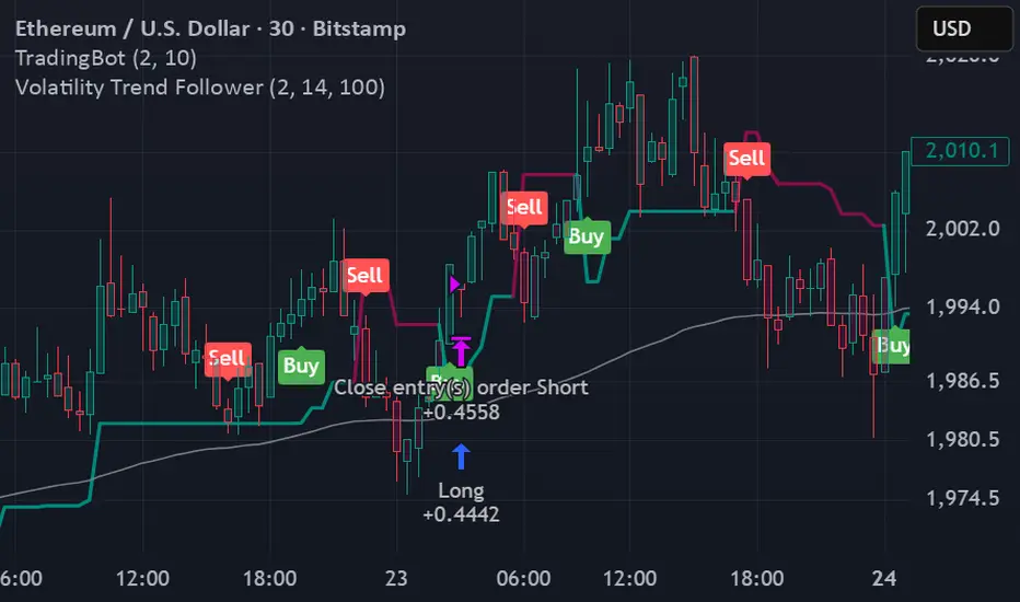
Volatility Trend FollowerThe script combines several classic technical analysis techniques:
SuperTrend / Adaptive Band - The main idea comes from the SuperTrend indicator, which uses ATR (Average True Range) to create a trailing band that adapts to volatility
ATR (Average True Range) - A volatility measure developed by J. Welles Wilder Jr.
EMA (Exponential Moving Average) - Used as a global trend filter
Heikin Ashi - An option to smooth prices and reduce noise

Elliott Wave Full Fractal System v2.0Elliott Wave Full Fractal System v2.0 – Q.C. FINAL (Guaranteed R/R)
Elliott Wave Full Fractal System is a multi-timeframe wave engine that automatically labels Elliott impulses and ABC corrections, then builds a rule-based, ATR-driven risk/reward framework around the “W3–W4–W5” leg.
“Guaranteed R/R” here means every order is placed with a predefined stop-loss and take-profit that respect a minimum Reward:Risk ratio – it does not mean guaranteed profits.
Core Idea
This strategy turns a full fractal Elliott Wave labelling engine into a systematic trading model.
It scans fractal pivots on three wave degrees (Primary, Intermediate, Minor) to detect 5-wave impulses and ABC corrections.
A separate “Trading Degree” pivot stream, filtered by a 200-EMA trend filter and ATR-based dynamic pivots, is then used to find W4 pullback entries with a minimum, user-defined Reward:Risk ratio.
Default Properties & Risk Assumptions
The backtest uses realistic but conservative defaults:
// Default properties used for backtesting
strategy(
"Elliott Wave Full Fractal System - Q.C. FINAL (Guaranteed R/R)",
overlay = true,
initial_capital = 10000, // realistic account size
default_qty_type = strategy.percent_of_equity,
default_qty_value = 1, // 1% risk per trade
commission_type = strategy.commission.cash_per_contract,
commission_value = 0.005, // example stock commission
slippage = 0 // see notes below
)
Account size: 10,000 (can be changed to match your own account).
Position sizing: 1% of equity per trade to keep risk per idea sustainable and aligned with TradingView’s recommendations.
Commission: 0.005 cash per contract/share as a realistic example for stock trading.
Slippage: set to 0 in code for clarity of “pure logic” backtesting. Real-life trading will experience slippage, so users should adjust this according to their market and broker.
Always re-run the backtest after changing any of these values, and avoid using high risk fractions (5–10%+) as that is rarely sustainable.
1. Full Fractal Wave Engine
The script builds and maintains four pivot streams using ATR-adaptive fractals:
Primary Degree (Macro Trend):
Captures the large swings that define the major trend. Labels ①–⑤ and ⒶⒷⒸ using blue “Circle” labels and thicker lines.
Intermediate Degree (Trading Degree):
Captures the medium swings (swing-trading horizon). Uses teal labels ( (1)…(5), (A)(B)(C) ).
Minor Degree (Micro Structure):
Tracks short-term swings inside the larger waves. Uses red roman numerals (i…v, a b c).
ABC Corrections (Optional):
When enabled, the engine tries to detect standard A–B–C corrective structures that follow a completed 5-wave impulse and plots them with dashed lines.
Each degree uses a dynamic pivot lookback that expands when ATR is above its EMA, so the system naturally requires “stronger” pivots in volatile environments and reacts faster in quiet conditions.
2. Theory Rules & Strict Mode
Normal Mode: More permissive detection. Designed to show more wave structures for educational / exploratory use.
Strict Mode: Enforces key Elliott constraints:
Wave 3 not shorter than waves 1 and 5.
No invalid W4 overlap with W1 (for standard impulses).
ABC Logic: After a confirmed bullish impulse, the script expects a down-up-down corrective pattern (A,B,C). After a bearish impulse, it looks for up-down-up.
3. Trend Filter & Pivots
EMA Trend Filter: A configurable EMA (default 200) is used as a non-wave trend filter.
Price above EMA → Only long setups are considered.
Price below EMA → Only short setups are considered.
ATR-Adaptive Pivots: The pivot engine scales its left/right bars based on current ATR vs ATR EMA, making waves and trading pivots more robust in volatile regimes.
4. Dynamic Risk Management (Guaranteed R/R Engine)
The trading engine is designed around risk, not just pattern recognition:
ATR-Based Stop:
Stop-loss is placed at:
Entry ± ATR × Multiplier (user-configurable, default 2.0).
This anchors risk to current volatility.
Minimum Reward:Risk Ratio:
For each setup, the script:
Computes the distance from entry to stop (risk).
Projects a take-profit target at risk × min_rr_ratio away from entry.
Only accepts the setup if risk is positive and the required R:R ratio is achievable.
Result: Every order is created with both TP and SL at a predefined distance, so each trade starts with a known, minimum Reward:Risk profile by design.
“Guaranteed R/R” refers exclusively to this order placement logic (TP/SL geometry), not to win-rate or profitability.
5. Trading Logic – W3–W4–W5 Pattern
The Trading pivot stream (separate from visual wave degrees) looks for a simple but powerful pattern:
Bullish structure:
Sequence of pivots forms a higher-high / higher-low pattern.
Price is above the EMA trend filter.
A strong “W3” leg is confirmed with structure rules (optionally stricter in Strict mode).
Entry (Long – W4 Pullback):
The “height” of W3 is measured.
Entry is placed at a configurable Fibonacci pullback (default 50%) inside that leg.
ATR-based stop is placed below entry.
Take-profit is projected to satisfy min Reward:Risk.
Bearish structure:
Mirrored logic (lower highs/lows, price below EMA, W3 down, W4 retrace up, W5 continuation down).
Once a valid setup is found, the script draws a colored box around the entry zone and a label describing the type of signal (“LONG SETUP” or “SHORT SETUP”) with the suggested limit price.
6. Orders & Execution
Entry Orders: The strategy uses limit orders at the computed W4 level (“Sniper Long” or “Sniper Short”).
Exits: A single strategy.exit() is attached to each entry with:
Take-profit at the projected minimum R:R target.
Stop-loss at ATR-based level.
One Trade at a Time: New setups are only used when there is no open position (strategy.opentrades == 0) to keep the logic clear and risk contained.
7. Visual Guide on the Chart
Wave Labels:
Primary: ①,②,③,④,⑤, ⒶⒷⒸ
Intermediate: (1)…(5), (A)(B)(C)
Minor: i…v, a b c
Trend EMA: Single blue EMA showing the dominant trend.
Setup Boxes:
Green transparent box → long entry zone.
Red transparent box → short entry zone.
Labels: “LONG SETUP / SHORT SETUP” labels mark the proposed limit entry with price.
8. How to Use This Strategy
Attach the strategy to your chart
Choose your market (stocks, indices, FX, crypto, futures, etc.) and timeframe (for example 1h, 4h, or Daily). Then add the strategy to the chart from your Scripts list.
Start with the default settings
Leave all inputs on their defaults first. This lets you see the “intended” behaviour and the exact properties used for the published backtest (account size, 1% risk, commission, etc.).
Study the wave map
Zoom in and out and look at the three wave degrees:
Blue circles → Primary degree (big picture trend).
Teal (1)…(5) → Intermediate degree (swing structure).
Red i…v → Minor degree (micro waves).
Use this to understand how the engine is interpreting the Elliott structure on your symbol.
Watch for valid setups
Look for the coloured boxes and labels:
Green box + “LONG SETUP” label → potential W4 pullback long in an uptrend.
Red box + “SHORT SETUP” label → potential W4 pullback short in a downtrend.
Only trades in the direction of the EMA trend filter are allowed by the strategy.
Check the Reward:Risk of each idea
For each setup, inspect:
Limit entry price.
ATR-based stop level.
Projected take-profit level.
Make sure the minimum Reward:Risk ratio matches your own rules before you consider trading it.
Backtest and evaluate
Open the Strategy Tester:
Verify you have a decent sample size (ideally 100+ trades).
Check drawdowns, average trade, win-rate and R:R distribution.
Change markets and timeframes to see where the logic behaves best.
Adapt to your own risk profile
If you plan to use it live:
Set Initial Capital to your real account size.
Adjust default_qty_value to a risk level you are comfortable with (often 0.5–2% per trade).
Set commission and slippage to realistic broker values.
Re-run the backtest after every major change.
Use as a framework, not a signal machine
Treat this as a structured Elliott/R:R framework:
Filter signals by higher-timeframe trend, major S/R, volume, or fundamentals.
Optionally hide some wave degrees or ABC labels if you want a cleaner chart.
Combine the system’s structure with your own trade management and discretion.
Best Practices & Limitations
This is an approximate Elliott Wave engine based on fractal pivots. It does not replace a full discretionary Elliott analysis.
All wave counts are algorithmic and can differ from a manual analyst’s interpretation.
Like any backtest, results depend heavily on:
Symbol and timeframe.
Sample size (more trades are better).
Realistic commission/slippage settings.
The 0-slippage default is chosen only to show the “raw logic”. In real markets, slippage can significantly impact performance.
No strategy wins all the time. Losing streaks and drawdowns will still occur even with a strict R:R framework.
Disclaimer
This script is for educational and research purposes only and does not constitute financial advice or a recommendation to buy or sell any security. Past performance, whether real or simulated, is not indicative of future results. Always test on multiple symbols/timeframes, use conservative risk, and consult your financial advisor before trading live capital.

US Market Long Horizon Momentum Summary in one paragraph
US Market Long Horizon Momentum is a trend following strategy for US index ETFs and futures built around a single eighteen month time series momentum measure. It helps you stay long during persistent bull regimes and step aside or flip short when long term momentum turns negative.
Scope and intent
• Markets. Large cap US equity indices, liquid US index ETFs, index futures
• Timeframes. 4h/ Daily charts
• Default demo used in the publication. SPY on 4h timeframe chart
• Purpose. Provide a minimal long bias index timing model that can reduce deep drawdowns and capture major cycles without parameter mining
• Limits. This is a strategy. Orders are simulated on standard candles only
Originality and usefulness
• Unique concept or fusion. One unscaled multiple month log return of an external benchmark symbol drives all entries and exits, with optional volatility targeting as a single risk control switch.
• Failure mode addressed. Fully passive buy and hold ignores the sign of long horizon momentum and can sit through multi year drawdowns. This script offers a way to step down risk in prolonged negative momentum without chasing short term noise.
• Testability. All parameters are visible in Inputs and the momentum series is plotted so users can verify every regime change in the Tester and on price history.
• Portable yardstick. The log return over a fixed window is a unit that can be applied to any liquid symbol with daily data.
Method overview in plain language
The method looks at how far the benchmark symbol has moved in log return terms over an eighteen month window in our example. If that long horizon return is positive the strategy allows a long stance on the traded symbol. If it is negative and shorts are enabled the strategy can flip short, otherwise it goes flat. There is an optional realised volatility estimate on the traded symbol that can scale position size toward a target annual volatility, but in the default configuration the model uses unit leverage and only the sign of momentum matters.
Base measures
Return basis. The core yardstick is the natural log of close divided by the close eighteen months ago on the benchmark symbol. Daily log returns of the traded symbol feed the realised volatility estimate when volatility targeting is enabled.
Components
• Component one Momentum eighteen months. Log of benchmark close divided by its close mom_lookback bars ago. Its sign defines the trend regime. No extra smoothing is applied beyond the long window itself.
• Component two Realised volatility optional. Standard deviation of daily log returns on the traded symbol over sixty three days. Annualised by the square root of 252. Used only when volatility targeting is enabled.
• Optional component Volatility targeting. Converts target annual volatility and realised volatility into a leverage factor clipped by a maximum leverage setting.
Fusion rule
The model uses a simple gate. First compute the sign of eighteen month log momentum on the benchmark symbol. Optionally compute leverage from volatility. The sign decides whether the strategy wants to be long, short, or flat. Leverage only rescales position size when enabled and does not change direction.
Signal rule
• Long suggestion. When eighteen month log momentum on the benchmark symbol is greater than zero, the strategy wants to be long.
• Short suggestion. When that log momentum is less than zero and shorts are allowed, the strategy wants to be short. If shorts are disabled it stays flat instead.
• Wait state. When the log momentum is exactly zero or history is not long enough the strategy stays flat.
• In position. In practice the strategy sits IN LONG while the sign stays positive and flips to IN SHORT or flat only when the sign changes.
Inputs with guidance
Setup
• Momentum Lookback (months). Controls the horizon of the log return on the benchmark symbol. Typical range 6 to 24 months. Raising it makes the model slower and more selective. Lowering it makes it more reactive and sensitive to medium term noise.
• Symbol. External symbol used for the momentum calculation, SPY by default. Changing it lets you time other indices or run signals from a benchmark while trading a correlated instrument.
Logic
• Allow Shorts. When true the strategy will open short positions during negative momentum regimes. When false it will stay flat whenever momentum is negative. Practical setting is tied to whether you use a margin account or an ETF that supports shorting.
Internal risk parameters (not exposed as inputs in this version) are:
• Target Vol (annual). Target annual volatility for volatility targeting, default 0.2.
• Vol Lookback (days). Window for realised volatility, default 63 trading days.
• Max Leverage. Cap on leverage when volatility targeting is enabled, default 2.
Usage recipes
Swing continuation
• Signal timeframe. Use the daily chart.
• Benchmark symbol. Leave at SPY for US equity index exposure.
• Momentum lookback. Eighteen months as a default, with twelve months as an alternative preset for a faster swing bias.
Properties visible in this publication
• Initial capital. 100000
• Base currency. USD
• Default order size method. 5% of the total capital in this example
• Pyramiding. 0
• Commission. 0.03 percent
• Slippage. 3 ticks
• Process orders on close. On
• Bar magnifier. Off
• Recalculate after order is filled. Off
• Calc on every tick. Off
• All request.security calls use lookahead = barmerge.lookahead_off
Realism and responsible publication
The strategy is for education and research only. It does not claim any guaranteed edge or future performance. All results in Strategy Tester are hypothetical and depend on the data vendor, costs, and slippage assumptions. Intrabar motion is not modeled inside daily bars so extreme moves and gaps can lead to fills that differ from live trading. The logic is built for standard candles and should not be used on synthetic chart types for execution decisions.
Performance is sensitive to regime structure in the US equity market, which may change over time. The strategy does not protect against single day crash risk inside bars and does not model gap risk explicitly. Past behavior of SPY and the momentum effect does not guarantee future persistence.
Honest limitations and failure modes
• Long sideways regimes with small net change over eighteen months can lead to whipsaw around the zero line.
• Very sharp V shaped reversals after deep declines will often be missed because the model waits for momentum to turn positive again.
• The sample size in a full SPY history is small because regime changes are infrequent, so any test must be interpreted as indicative rather than statistically precise.
• The model is highly dependent on the chosen lookback. Users should test nearby values and validate that behavior is qualitatively stable.
Legal
Education and research only. Not investment advice. You are responsible for your own decisions. Always test on historical data and in simulation with realistic costs before any live use.

Bollinger Bands Mean Reversion using RSI [Krishna Peri]How it Works
Long entries trigger when:
- RSI reaches oversold levels, and
- At least one bullish candle closes inside the lower Bollinger Band
Short entries trigger when:
- RSI reaches overbought levels, and
- At least one bearish candle closes inside the upper Bollinger Band
This approach aims to capture exhaustion moves where price pushes into extreme deviation from its mean and then snaps back toward the middle band.
Important Disclaimer
This is a mean-reversion strategy, which means it performs best in sideways, ranging, or slowly oscillating market conditions. When markets shift into strong trends, Bollinger Bands expand and volatility increases, which may cause some signals to become inaccurate or fail altogether.
For best results, combine this script with:
- Price action
- Market structure
- Higher-timeframe trend context
- Previous day/week/month highs & lows
- Untested liquidity levels or imbalance zones
- Session timing (Asia, London, NY)
Using these confluences helps filter out low-probability trades and significantly improves consistency and precision.
Robrechtian Long-Medium Breakout Trend SystemRobrechtian Long–Medium-Term Breakout Trend System
A professional, rule-based trend-following strategy designed to capture large, sustained price movements using pure price action and breakouts.
This system follows long-established trend-following philosophy: no prediction, no volatility targeting, and no profit targets. Only disciplined entries, position additions, and exits driven entirely by trend structure.
Core Principles
Breakout-driven entries: Initial positions are taken only when price breaks above/below the 80-day Donchian channel, confirming a long–medium-term trend shift.
Short-term confirmation: Breakouts must also exceed the 20-day channel, reducing false positives.
Trend-direction filter: A 50-day moving average slope filter ensures alignment with the broader trend.
Explosive bar filter: Entries avoid excessively large, single-candle expansions (>2.5× ATR(20)) to prevent chasing exhaustion spikes.
Pyramiding into strength: Additional units are added only when price makes fresh 20-day breakouts in the direction of the trend. No scaling out. No adding on dips.
Exit only on trend violation: Positions are closed exclusively when price breaks the opposite 80-day channel. This preserves unlimited upside while enforcing disciplined exits.
Pure trend philosophy: No volatility targeting, no smoothing, no discretionary overrides, no optimization for short-term performance.
Intended Use
This system is designed primarily for diversified futures portfolios, where diversification across dozens of globally liquid markets creates robustness and stability. However, it may also be used on individual assets for educational and analytical purposes.
The system embraces the core trend-following logic:
Small losses, big winners, and unlimited upside when trends persist.
⚠️ WARNINGS / DISCLAIMERS
⚠️ Warning 1 — This strategy is not optimized for single stocks
The Robrechtian Trend System is designed for multi-asset futures portfolios, not single equities.
Performance on individual tickers may vary greatly due to lack of diversification.
⚠️ Warning 2 — Trend following includes substantial drawdowns
Deep drawdowns are a normal and expected feature of all long-term trend-following systems.
The strategy does not attempt to smooth returns or manage volatility.
If you seek steady, low-volatility equity curves, this system is not suitable.
⚠️ Warning 3 — No volatility targeting or risk smoothing
This system intentionally avoids volatility-based position sizing.
Trades may experience larger fluctuations than systems using risk parity or vol targeting.
⚠️ Warning 4 — Not financial advice
This script is for educational and research purposes only.
Past performance does not guarantee future results.
Use at your own risk.
⚠️ Warning 5 — TradingView backtests have known limitations
TradingView does not simulate:
futures contract roll logic
slippage
real bid/ask spreads
liquidity conditions
limit-up/limit-down behavior
Results may vary from live market execution.

Triple EMA + RSI + ATRThis comprehensive trading system combines triple EMA alignment, RSI momentum filtering, and dynamic ATR-based risk management. The strategy enters positions only when fast, medium, and slow EMAs align in proper order (bullish or bearish), confirmed by RSI remaining within defined thresholds (not overbought/oversold) and a volume spike above its moving average. Exits are managed intelligently using a multi-tier approach: a fixed stop-loss based on ATR, a first profit target at a predefined risk-reward ratio, and a trailing stop that activates after reaching a second, higher profit tier. Designed for trend-following with built-in momentum and volume confirmation, it features professional order execution with configurable commission and slippage for realistic backtesting. Visual cues including colored backgrounds and signal shapes enhance chart clarity.

XRP Non-Stop Strategy (TP 25% / SL 15%)XRP Non-Stop Strategy (TP 25% / SL 15%) is a continuous long-side trading system designed specifically for XRP. The strategy uses an EMA-based trend filter (EMA20/EMA50) to confirm bullish conditions before entering a long position. Each trade applies a fixed +25% Take Profit target and a −15% Stop Loss, calculated dynamically from the entry price.
When a trade closes—whether by TP or SL—the strategy automatically re-enters on the next qualifying signal, enabling uninterrupted position cycling.
Features include:
• EMA-based trend confirmation
• Dynamic TP/SL visualization on the chart
• Clear BUY and EXIT markers
• Dedicated alert conditions for automation

XRP Non-Stop Strategy (TP 25% / SL 15%)This strategy performs continuous automated trading exclusively on XRP. It opens long positions during favorable trend conditions, using a fixed Take Profit target of 25% above the entry price and a fixed Stop Loss of 15% below the entry. Once a trade is closed (either TP or SL), the strategy automatically re-enters on the next valid signal, enabling uninterrupted trading.
The script includes:
Dynamic Take Profit & Stop Loss lines
Optional EMA trend filter
Visual BUY and EXIT markers
TradingView alerts for automation or notifications
This strategy is built for traders who want a simple, price-action-driven system without fixed price levels, relying only on percentage-based movement from each entry.

Strategy: HMA 50 + Supertrend SniperHMA 50 + Supertrend Confluence Strategy (Trend Following with Noise Filtering)
Description:
Introduction and Concept This strategy is designed to solve a common problem in trend-following trading: Lag vs. False Signals. Standard Moving Averages often lag too much, while price action indicators can generate false signals during choppy markets. This script combines the speed of the Hull Moving Average (HMA) with the volatility-based filtering of the Supertrend indicator to create a robust "Confluence System."
The primary goal of this script is not just to overlay two indicators, but to enforce a strict rule where a trade is only taken when Momentum (HMA) and Volatility Direction (Supertrend) are in perfect agreement.
Why this combination? (The Logic Behind the Mashup)
Hull Moving Average (HMA 50): We use the HMA because it significantly reduces lag compared to SMA or EMA by using weighted calculations. It acts as our primary Trend Direction detector. However, HMA can be too sensitive and "whipsaw" during sideways markets.
Supertrend (ATR-based): We use the Supertrend (Factor 3.0, Period 10) as our Volatility Filter. It uses Average True Range (ATR) to determine the significant trend boundary.
How it Works (Methodology) The strategy uses a boolean logic system to filter out low-quality trades:
Bullish Confluence: The HMA must be rising (Slope > 0) AND the Close Price must be above the Supertrend line (Uptrend).
Bearish Confluence: The HMA must be falling (Slope < 0) AND the Close Price must be below the Supertrend line (Downtrend).
The "Choppy Zone" (Noise Filter): This is a unique feature of this script. If the HMA indicates one direction (e.g., Rising) but the Supertrend indicates the opposite (e.g., Downtrend), the market is considered "Choppy" or indecisive. In this state, the script paints the candles or HMA line Gray and exits all positions (optional setting) to preserve capital.
Visual Guide & Signals To make the script easy to interpret for traders who do not read Pine Script, I have implemented specific visual cues:
Green Cross (+): Indicates a LONG entry signal. Both HMA and Supertrend align bullishly.
Red Cross (X): Indicates a SHORT entry signal. Both HMA and Supertrend align bearishly.
Thick Line (HMA): The main line changes color based on the trend.
Green: Bullish Confluence.
Red: Bearish Confluence.
Gray: Divergence/Choppy (No Trade Zone).
Thin Step Line: This is the Supertrend line, serving as your dynamic Trailing Stop Loss.
Strategy Settings
HMA Length: Default is 50 (Mid-term trend).
ATR Factor/Period: Default is 3.0/10 (Standard for trend catching).
Exit on Choppy: A toggle switch allowing users to decide whether to hold through noise or exit immediately when indicators disagree.
Risk Warning This strategy performs best in trending markets (Forex, Crypto, Indices). Like all trend-following systems, it may experience drawdown during prolonged accumulation/distribution phases. Please backtest with your specific asset before using it with real capital.

Oleg_Aryukov_StrategyTrader Oleg Aryukov's strategy, based on a variety of oscillators, allows him to try to catch reversals in cryptocurrencies.

AliceTears GridAliceTears Grid is a customizable Mean Reversion system designed to capitalize on market volatility during specific trading sessions. Unlike standard grid bots that place blind limit orders, this strategy establishes a daily or session-based "Baseline" and looks for price over-extensions to fade the move back to the mean.
This strategy is best suited for ranging markets (sideways accumulation) or specific forex sessions (e.g., Asian Session or NY/London overlap) where price tends to revert to the opening price.
🛠 How It Works
1. The Baseline & Grid Generation At the start of every session (or the daily open), the script records the Open price. It then projects visual grid lines above and below this price based on your Step % input.
Example: If the Open is $100 and Step is 1%, lines are drawn at $101, $102, $99, $98, etc.
2. Entry Logic: Reversal Mode This script features a "Reversal Mode" (enabled by default) to filter out "falling knives."
Standard Grid: Buys immediately when price touches the line.
AliceTears Logic: Waits for the price to breach a grid level and then close back inside towards the mean. This confirms a potential rejection of that level before entering.
3. Exit Logic
Target Profit: The primary target is the previous grid level (Mean Reversion).
Trailing Stop: If the price continues moving in your favor, a trailing stop activates to maximize the run.
Stop Loss: A manual percentage-based stop loss is available to prevent deep drawdowns in trending markets.
⚙️ Key Features
Visual Grid: Automatically draws entry levels on the chart for the current session, helping you visualize where the "math" is waiting for price.
Timezone & Session Control: Includes a custom Timezone Offset tool. You can trade specific hours (e.g., 09:30–16:00) regardless of your chart's UTC setting.
Grid Management: Independent logic for Long and Short grids with pyramiding capabilities.
Safety Filters: Options to force-close trades at the end of the session to avoid overnight gaps.
⚠️ Risk Warning
Please Read Before Using: This is a Counter-Trend / Grid Strategy.
Pros: High win rate in sideways/ranging markets.
Cons: In strong trending markets (parabolic pumps or crashes), this strategy will add to losing positions ("catch a falling knife").
Recommendation: Always use the Stop Loss and Date Filter inputs. Do not run this on highly volatile assets without strict risk management parameters.
Settings Guide
Entry Reversal Mode: Keep checked for safer entries. Uncheck for aggressive limit-order style execution.
Grid Step (%): The distance between lines. For Forex, use lower values (0.1% - 0.5%). For Crypto, use higher values (1.0% - 3.0%).
UTC Offset: Adjust this to align the Session Hours with your target market (e.g., -5 for New York).
This script is open source. Feel free to use it for educational purposes or modify it to fit your trading style.

Dynamic Ratchet Trend Strategy [VIX Filter]Overview This strategy is a long-only trend-following system designed to capture major market moves while strictly managing downside risk through a state-machine based "Ratchet" exit logic. It incorporates a volatility filter using the CBOE VIX index to stay out of (or exit) the market during high-stress environments.
Key Features
1. Multi-Condition Entries The strategy looks for momentum shifts and trend breakouts using four Simple Moving Averages (25, 50, 100, 200).
Momentum Cross: SMA 25 crossover above SMA 50.
Trend Breakouts: A specific "3-Bar Breakout" logic above the SMA 50, 100, or 200. This requires the price to hold above the SMA for 3 consecutive bars after being below it, reducing false signals compared to simple closes.
2. VIX Volatility Filter Before entering any trade, the script checks the CBOE:VIX.
Filter: If VIX is above the threshold (default 32), new entries are blocked.
Panic Exit: If you are in a position and the VIX spikes above the threshold, the strategy executes an immediate "Panic Exit" to preserve capital during market crashes.
3. The "Ratchet" Exit System (3 Stages) Unlike a standard trailing stop, this strategy uses a 3-stage dynamic exit mechanism that tightens as profits grow:
Stage 0 (Initial Risk): Standard percentage-based Stop Loss from the entry price.
Stage 1 (The Lock-In): Triggered when profit hits 10% (configurable).
Unique Logic: Instead of trailing from the highest high, the stop is calculated based on the price at the exact moment this stage was triggered. It "steps up" once and holds, securing the initial move without being prematurely stopped out by normal volatility.
Stage 2 (Trailing Mode): Triggered when profit hits 15% (configurable).
The strategy switches to a classic Trailing Stop, following the percentage distance from the Highest High.
4. Emergency Backup A "Dead Cross" (SMA 25 crossing under SMA 50) acts as a final fail-safe to close positions if the trend reverses completely before hitting a stop.
Settings & Inputs
SMAs: Customize the lengths for all four moving averages.
VIX Filter: Toggle the filter on/off and set the panic threshold.
Exit Logic: Fully customizable percentages for Initial SL, Stage 1 Trigger/Distance, and Stage 2 Trigger/Trailing Distance.
Disclaimer This script is for educational purposes only. Past performance is not indicative of future results. Always manage your risk appropriately.

Ratchet Exit Trend Strategy with VIX FilterThis strategy is a trend-following system designed specifically for volatile markets. Instead of focusing solely on the "perfect entry," this script emphasizes intelligent trade management using a custom **"Ratchet Exit System."**
Additionally, it integrates a volatility filter based on the CBOE Volatility Index (VIX) to minimize risk during extreme market phases.
### 🎯 The Concept: Ratchet Exit
The "Ratchet" system operates like a mechanical ratchet tool: the Stop Loss can only move in one direction (up, for long trades) and "locks" into specific stages. The goal is to give the trade "room to breathe" initially to avoid being stopped out by noise, then aggressively reduce risk as the trade moves into profit.
The exit logic moves through 3 distinct phases:
1. **Phase 0 (Initial Risk):** At the start of the trade, a wide Stop Loss is set (Default: 10%) to tolerate normal market volatility.
2. **Phase 1 (Risk Reduction):** Once the trade reaches a specific floating profit (Default: +10%), the Stop Loss is raised and "pinned" to a fixed value (Default: -8% from entry). This drastically reduces risk while keeping the trade alive.
3. **Phase 2 (Trailing Mode):** If the trend extends to a higher profit zone (Default: +15%), the Stop switches to a dynamic Trailing Mode. It follows the **Highest High** at a fixed percentage distance (Default: 8%).
### 🛡️ VIX Filter & Panic Exit
High volatility is often the enemy of trend-following strategies.
* **Entry Filter:** The system will not enter new positions if the VIX is above a user-defined threshold (Default: 32). This helps avoid entering "falling knife" markets.
* **Panic Exit:** If the VIX spikes above the threshold (32) while a trade is open, the position is closed immediately to protect capital (Emergency Exit).
### 📈 Entry Signals
The strategy trades **LONG only** and uses Simple Moving Averages (SMAs) to identify trends:
* **Golden Cross:** SMA 25 crosses over SMA 50.
* **3-Bar Breakouts:** A confirmation logic where the price must close above the SMA 50, 100, or 200 for 3 consecutive bars.
### ⚙️ Settings (Inputs)
All parameters are fully customizable via the settings menu:
* **SMAs:** Lengths for the trend indicators (Default: 25, 50, 100, 200).
* **VIX Filter:** Toggle the filter on/off and adjust the panic threshold.
* **Ratchet Settings:** Percentages for Initial Stop, Trigger Levels for Stages 1 & 2, and the Trailing Distance.
### ⚠️ Technical Note & Risk Warning
This script uses `request.security` to fetch VIX data. Please ensure you understand the risks associated with trading leveraged or volatile assets. Past performance is not indicative of future results.

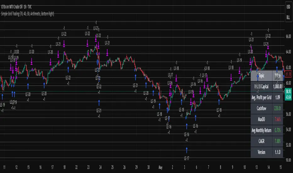
Simple Grid Trading v1.0 [PUCHON]Simple Grid Trading v1.0
Overview
This is a Long-Only Grid Trading Strategy developed in Pine Script v6 for TradingView. It is designed to profit from market volatility by placing a series of Buy Limit orders at predefined price levels. As the price drops, the strategy accumulates positions. As the price rises, it sells these positions at a profit.
Features
Grid Types : Supports both Arithmetic (equal price spacing) and Geometric (equal percentage spacing) grids.
Flexible Order Management : Uses strategy.order for precise control and prevents duplicate orders at the same level.
Performance Dashboard : A real-time table displaying key metrics like Capital, Cashflow, and Drawdown.
Advanced Metrics : Includes Max Drawdown (MaxDD) , Avg Monthly Return , and CAGR calculations.
Customizable : Fully adjustable price range, grid lines, and lot size.
Dashboard Metrics
The dashboard (default: Bottom Right) provides a quick snapshot of the strategy's performance:
Initial Capital : The starting capital defined in the strategy settings.
Lot Size : The fixed quantity of assets purchased per grid level.
Avg. Profit per Grid : The average realized profit for each closed trade.
Cashflow : The total realized net profit (closed trades only).
MaxDD : Maximum Drawdown . The largest percentage drop in equity (realized + unrealized) from a peak.
Avg Monthly Return : The average percentage return generated per month.
CAGR : Compound Annual Growth Rate . The mean annual growth rate of the investment over the specified time period.
Strategy Settings (Inputs)
Grid Settings
Upper Price : The highest price level for the grid.
Lower Price : The lowest price level for the grid.
Number of Grid Lines : The total number of levels (lines) in the grid.
Grid Type :
Arithmetic: Distance between lines is fixed in price terms (e.g., $10, $20, $30).
Geometric: Distance between lines is fixed in percentage terms (e.g., 1%, 2%, 3%).
Lot Size : The fixed amount of the asset to buy at each level.
Dashboard Settings
Show Dashboard : Toggle to hide/show the performance table.
Position : Choose where the dashboard appears on the chart (e.g., Bottom Right, Top Left).
How It Works
Initialization : On the first bar, the script calculates the price levels based on your Upper/Lower price and Grid Type.
Entry Logic :
The strategy places Buy Limit orders at every grid level below the current price.
It checks if a position already exists at a specific level to avoid "stacking" multiple orders on the same line.
Exit Logic :
For every Buy order, a corresponding Sell Limit (Take Profit) order is placed at the next higher grid level.
MaxDD Calculation :
The script continuously tracks the highest equity peak.
It calculates the drawdown on every bar (including intra-bar movements) to ensure accuracy.
Displayed as a percentage (e.g., 5.25%).
Disclaimer
This script is for educational and backtesting purposes only. Grid trading involves significant risk, especially in strong trending markets where the price may move outside your grid range. Always use proper risk management.
MTF EMA Hariss 369The strategy has been prepared in a simplistic manner and easy to understand the concept by any novice trader.
Indicators used:
Current Time frame 20 EMA- Gives clear look about current time frame dynamic support and resistance and trend as well.
Higher Time Frame 20 EMA: Gives macro level trend, support and resistance
Kama: Capture volatility and trend direction.
RVOL: Main factor of price movement.
Buy when price closes above current time frame 20 ema and current time frame 20 ema is above higher time frame 20 ema. Stop loss just below the low of last candle. One can use current time frame 20 ema, higher time frame 20 ema or kama as stop loss depending upon type of asset class and risk appetite. The ideal way is to keep 20 ema as trailing sl if one wants to trail with trend.
Sell when price closes below current time frame 20 ema and current time frame 20 ema is lower than higher time frame 20 ema. Stop loss just above high of last candle.
Ideal target is 1.5 or 2 times of stop loss.
Entry and exit time depends on trading style. Eg. if you want to enter and exit in 5 min time frame, then choose 15 min or 1h as higher time frame as trend filter. Buy and sell signals are also plotted based on this strategy. One should always go with the higher time frame trend. Opting higher time frame trend filter always filters out market noises.
