Moon Phases & Declinations - Chronos Capital [BETA]High-Precision Lunar Cycles: Moon Phases & Declinations (Swiss Ephemeris)
Overview
This indicator provides institutional-grade astronomical data directly on your chart. Unlike standard scripts that use basic sine-wave approximations, this tool implements the **Swiss Ephemeris algorithm**, the gold standard for high-precision celestial calculations.
By tracking the Moon’s phases and its **Maximum/Minimum Declinations**, traders can identify potential "turning points" or "energy shifts" in market volatility often associated with lunar cycles.
---
Key Features
Ultra-High Precision: Calculations are accurate to within *seconds* of time, ensuring that the visual plot aligns perfectly with astronomical reality.
Moon Phase Tracking: Distinct markers for New Moon, Full Moon, and Quarters.
Lunar Declination Peaks: Automatically identifies when the moon reaches its *Maximum North* and *Maximum South* points (Lunar Extremes).
Customizable Visuals: Toggle between background highlights, vertical lines, or plot signals to suit your trading style.
---
Technical Accuracy
This script is built using a ported version of the Swiss Ephemeris
Positional Accuracy: Within 0.1 arcseconds.
Time Accuracy: Within **~1-2 seconds** of official JPL data.
Algorithm: Integration of the *ELP2000-85* lunar theory for maximum reliability over decades of historical data.
---
### **How to Use**
1. **Reversal Zones:** Watch for the Moon’s *Max/Min Declination* points, which often coincide with local tops or bottoms in trending markets.
2. **Volatility Shifts:** Use the *New Moon* and *Full Moon* markers to anticipate periods of increased or decreased market liquidity and volume.
3. **Confluence:** Best used in combination with your existing price action or momentum indicators to add a "time-based" filter to your entries.
*Disclaimer: This tool is for educational and analytical purposes only. Lunar cycles are a study of time-based correlation, not a guaranteed financial signal.*
Forecasting

Latent Energy Reactor [The_lurker]Latent Energy Reactor | مفاعل الطاقة الكامنة
═════════════════════════════════════════════════════════════
🔬 THE PHILOSOPHY
═════════════════════════════════════════════════════════════
Markets operate in cycles of compression and expansion. Before every significant price movement, there exists a period where buyers and sellers reach a temporary equilibrium — a consolidation zone where energy accumulates like pressure building in a reactor.
The Latent Energy Reactor was designed to identify these critical zones, measure the energy building within them, and predict the direction of the inevitable breakout.
This indicator transforms the abstract concept of "market energy" into a quantifiable, visual system that traders can use to anticipate high-probability breakout opportunities.
═════════════════════════════════════════════════════════════
🎯 THE THREE BOX STATES
═════════════════════════════════════════════════════════════
Understanding the three box states is crucial for proper interpretation:
📦 STATE 1: ACTIVE ZONE (GRAY BOX)
─────────────────────────────────────
Visual Characteristics:
• Color: Gray/Neutral with 3D depth effect
• Extends to the right edge of the chart (future projection)
• Contains pressure lines (dotted horizontal lines inside)
• Displays gravity center line (dashed line showing volume-weighted center)
• Energy progress bar beneath the box
• Real-time information panel appears on screen
What It Means:
The gray box represents a LIVE consolidation zone currently forming. Price is contained within the boundaries, and energy is actively accumulating. This is the "waiting phase" where the reactor is charging.
What to Watch:
• Energy percentage climbing toward critical levels (80%+)
• Gravity center position (upper half = bullish bias, lower half = bearish bias)
• Top and bottom rejection counts in the information panel
• Phase progression (Forming → Growth → Mature → Exhaustion)
Trading Approach:
Do NOT trade inside the gray box. This is the preparation phase. Monitor the energy levels and predicted direction, but wait for confirmation.
📦 STATE 2: BULLISH BREAKOUT BOX (GREEN BOX)
─────────────────────────────────────────────
Visual Characteristics:
• Color: Green with 3D depth effect
• Box boundaries are now fixed (no longer extending right)
• Displays "BUY" text centered inside the box
• Stop Loss line appears below the box (orange)
• Three Take Profit lines appear above (teal/cyan)
• Entry line at the box's upper boundary (white dashed)
What It Means:
The green box indicates a CONFIRMED bullish breakout. Price has broken above the consolidation zone's upper boundary, releasing the accumulated energy upward.
Automatic Calculations Displayed:
• Entry Price: Upper boundary of the box
• Stop Loss: Lower boundary minus ATR buffer
• TP1: Entry + (Risk × 1.0) — 1:1 reward ratio
• TP2: Entry + (Risk × 1.5) — 1.5:1 reward ratio
• TP3: Entry + (Risk × 2.0) — 2:1 reward ratio
Trading Approach:
Consider long positions with the displayed SL/TP levels as guidelines. The higher the energy level and breakout quality score were before the breakout, the more reliable the signal.
📦 STATE 3: BEARISH BREAKOUT BOX (RED BOX)
──────────────────────────────────────────
Visual Characteristics:
• Color: Red with 3D depth effect
• Box boundaries are now fixed
• Displays "SELL" text centered inside the box
• Stop Loss line appears above the box (orange)
• Three Take Profit lines appear below (teal/cyan)
• Entry line at the box's lower boundary (white dashed)
What It Means:
The red box indicates a CONFIRMED bearish breakout. Price has broken below the consolidation zone's lower boundary, releasing the accumulated energy downward.
Automatic Calculations Displayed:
• Entry Price: Lower boundary of the box
• Stop Loss: Upper boundary plus ATR buffer
• TP1: Entry - (Risk × 1.0) — 1:1 reward ratio
• TP2: Entry - (Risk × 1.5) — 1.5:1 reward ratio
• TP3: Entry - (Risk × 2.0) — 2:1 reward ratio
Trading Approach:
Consider short positions with the displayed SL/TP levels as guidelines. Stronger setups have higher pre-breakout energy and quality scores.
═════════════════════════════════════════════════════════════
⚛️ THE ENERGY CALCULATION SYSTEM
═════════════════════════════════════════════════════════════
The energy percentage (0-100%) is calculated using four factors:
Compression Score (up to 40 points)
Measures how tight the range is relative to normal volatility (ATR). Tighter compression = higher energy storage.
Time Score (up to 35 points)
Longer consolidation periods accumulate more energy. Each bar adds to the score up to the maximum.
Maturity Bonus (up to 15 points)
Zones that reach mature phases receive bonus energy points, recognizing that extended consolidations often produce more powerful breakouts.
Tightness Bonus (up to 10 points)
Extra points awarded when the range height is exceptionally small relative to ATR.
═════════════════════════════════════════════════════════════
📊 THE GRAVITY CENTER SYSTEM
═════════════════════════════════════════════════════════════
How It Works:
The gravity center is the volume-weighted average price within the consolidation zone. It reveals where the majority of trading activity (and thus institutional interest) is concentrated.
Interpretation:
• Gravity center in UPPER half → Institutions accumulating → Bullish bias
• Gravity center in LOWER half → Institutions distributing → Bearish bias
• Gravity center at MIDDLE → Neutral/Uncertain
Visual Display:
A dashed line with a ⚖️ symbol marks the gravity center inside active zones. The line color matches the directional bias.
═════════════════════════════════════════════════════════════
🏦 INSTITUTIONAL FOOTPRINT DETECTION
═════════════════════════════════════════════════════════════
What It Measures:
The indicator scans for volume anomalies — bars where volume significantly exceeds the average while price remains contained within the zone.
Why It Matters:
Large volume without price movement often indicates institutional players building positions. They cannot accumulate or distribute large quantities without leaving a "footprint" in the volume data.
Score Interpretation:
• Below 30%: Normal retail activity
• 30-50%: Some institutional interest detected
• Above 50%: Significant institutional footprint (marked with 🏦 icon)
═════════════════════════════════════════════════════════════
📈 MATURITY PHASES
═════════════════════════════════════════════════════════════
⚒ Forming Phase
The zone has just been identified. Energy is low, and the pattern needs more time to develop. Premature breakouts during this phase have higher failure rates.
📈 Growth Phase
The zone is developing nicely. Energy is building, and the consolidation pattern is becoming more defined. Watch for increasing rejection counts at boundaries.
✅ Mature Phase
Optimal trading phase. The zone has accumulated significant energy, institutional footprints are often visible, and breakout quality scores are typically highest.
⚠ Exhaustion Phase
The zone has persisted beyond typical duration. While energy remains high, the pattern may be losing its predictive power.
═════════════════════════════════════════════════════════════
🎨 VISUAL ELEMENTS GUIDE
═════════════════════════════════════════════════════════════
3D Box Effect
The 3D rendering creates visual depth with a top face and side face, making boxes stand out clearly. Adjustable via "3D Depth" and "3D Height %" settings.
Pressure Lines
Dotted horizontal lines inside active zones visualize internal pressure distribution. Lines closer to the gravity center are more opaque.
Energy Progress Bar
A horizontal bar beneath each zone shows energy level visually. Color progresses: green (low) → yellow (moderate) → orange (high) → red (critical).
Imminent Breakout Warning
When energy reaches critical threshold (default 80%), a warning label "⚠ IMMINENT!" appears above the active zone.
Information Panel
Real-time table displaying: Energy Level, Phase, Prediction, Breakout Quality, Institutional Footprint, Top/Bottom Rejections.
═════════════════════════════════════════════════════════════
📊 READING THE SIGNALS
═════════════════════════════════════════════════════════════
Energy Levels:
• Below 40%: Low energy — breakout unlikely soon
• 40-60%: Moderate energy — zone developing
• 60-80%: High energy — prepare for potential breakout
• Above 80%: Critical energy — breakout imminent
Breakout Quality Score:
• Below 50%: Weak setup — higher false breakout risk
• 50-70%: Moderate setup — proceed with caution
• Above 70%: Strong setup — high probability trade
Direction Confidence:
• Below 55%: Neutral — wait for clearer signals
• 55-70%: Moderate confidence
• Above 70%: High confidence prediction
═════════════════════════════════════════════════════════════
⚙️ RECOMMENDED SETTINGS
═════════════════════════════════════════════════════════════
For Scalping (1-15 min):
Min Bars in Range: 10-15 | ATR Period: 10 | Range ATR Multiplier: 2.0
For Day Trading (15min-1H):
Min Bars in Range: 15-20 | ATR Period: 14 | Range ATR Multiplier: 2.5
For Swing Trading (4H-Daily):
Min Bars in Range: 20-30 | ATR Period: 20 | Range ATR Multiplier: 3.0
═════════════════════════════════════════════════════════════
🔔 ALERTS
═════════════════════════════════════════════════════════════
• New Zone Alert: Triggers when a new consolidation zone is identified
• Imminent Breakout Alert: Triggers when energy reaches critical levels
• Bullish Breakout Alert: Triggers on confirmed bullish breakout
• Bearish Breakout Alert: Triggers on confirmed bearish breakout
═════════════════════════════════════════════════════════════
⚠️ DISCLAIMER
═════════════════════════════════════════════════════════════
This indicator is designed as a technical analysis tool to identify consolidation patterns and anticipate potential breakout directions. No indicator can predict the future with certainty. The displayed SL/TP levels are suggestions based on mathematical calculations, not guarantees.
This indicator is for educational and analytical purposes only. It does not constitute financial, investment, or trading advice. Use it in conjunction with your own strategy and risk management. Neither TradingView nor the developer is liable for any financial decisions or losses.
═════════════════════════════════════════════════════════════
═════════════════════════════════════════════════════════════
مفاعل الطاقة الكامنة | Latent Energy Reactor
🔬 الفلسفة
═════════════════════════════════════════════════════════════
تعمل الأسواق في دورات من الضغط والتمدد. قبل كل حركة سعرية كبيرة، توجد فترة يصل فيها المشترون والبائعون إلى توازن مؤقت — منطقة تجميع حيث تتراكم الطاقة مثل الضغط المتراكم في مفاعل.
صُمم مفاعل الطاقة الكامنة لتحديد هذه المناطق الحرجة، وقياس الطاقة المتراكمة داخلها، والتنبؤ باتجاه الاختراق الحتمي.
يحوّل هذا المؤشر المفهوم المجرد لـ "طاقة السوق" إلى نظام قابل للقياس والعرض البصري يمكن للمتداولين استخدامه لتوقع فرص الاختراق عالية الاحتمالية.
═════════════════════════════════════════════════════════════
🎯 حالات الصندوق الثلاث
═════════════════════════════════════════════════════════════
فهم حالات الصندوق الثلاث ضروري للتفسير الصحيح:
📦 الحالة الأولى: المنطقة النشطة (الصندوق الرمادي)
─────────────────────────────────────────────────────
الخصائص البصرية:
• اللون: رمادي/محايد مع تأثير عمق ثلاثي الأبعاد
• يمتد إلى الحافة اليمنى للرسم البياني (إسقاط مستقبلي)
• يحتوي على خطوط الضغط (خطوط أفقية منقطة بالداخل)
• يعرض خط مركز الثقل (خط متقطع يُظهر المركز المرجح بالحجم)
• شريط تقدم الطاقة أسفل الصندوق
• تظهر لوحة المعلومات الفورية على الشاشة
ماذا يعني:
الصندوق الرمادي يمثل منطقة تجميع حَيّة تتشكل حالياً. السعر محتوى داخل الحدود، والطاقة تتراكم بنشاط. هذه هي "مرحلة الانتظار" حيث المفاعل يشحن.
ما يجب مراقبته:
• نسبة الطاقة تصعد نحو المستويات الحرجة (80%+)
• موقع مركز الثقل (النصف العلوي = ميل صعودي، النصف السفلي = ميل هبوطي)
• عدد الرفض العلوي والسفلي في لوحة المعلومات
• تقدم المرحلة (تشكّل ← نمو ← نضج ← إرهاق)
نهج التداول:
لا تتداول داخل الصندوق الرمادي. هذه مرحلة الإعداد. راقب مستويات الطاقة والاتجاه المتوقع، لكن انتظر التأكيد.
📦 الحالة الثانية: صندوق الاختراق الصعودي (الصندوق الأخضر)
─────────────────────────────────────────────────────────────
الخصائص البصرية:
• اللون: أخضر مع تأثير عمق ثلاثي الأبعاد
• حدود الصندوق ثابتة الآن (لم تعد تمتد لليمين)
• يعرض نص "شراء" أو "BUY" في منتصف الصندوق
• يظهر خط وقف الخسارة أسفل الصندوق (برتقالي)
• تظهر ثلاثة خطوط أهداف فوق الصندوق (فيروزي)
• خط الدخول عند الحد العلوي للصندوق (أبيض متقطع)
ماذا يعني:
الصندوق الأخضر يشير إلى اختراق صعودي مُؤَكَّد. كسر السعر فوق الحد العلوي لمنطقة التجميع، محرراً الطاقة المتراكمة للأعلى.
الحسابات التلقائية المعروضة:
• سعر الدخول: الحد العلوي للصندوق
• وقف الخسارة: الحد السفلي ناقص حاجز ATR
• الهدف 1: الدخول + (المخاطرة × 1.0) — نسبة مكافأة 1:1
• الهدف 2: الدخول + (المخاطرة × 1.5) — نسبة مكافأة 1.5:1
• الهدف 3: الدخول + (المخاطرة × 2.0) — نسبة مكافأة 2:1
نهج التداول:
فكر في صفقات شراء مع مستويات وقف الخسارة والأهداف المعروضة كإرشادات. كلما ارتفع مستوى الطاقة ودرجة جودة الاختراق قبل الكسر، كانت الإشارة أكثر موثوقية.
📦 الحالة الثالثة: صندوق الاختراق الهبوطي (الصندوق الأحمر)
─────────────────────────────────────────────────────────────
الخصائص البصرية:
• اللون: أحمر مع تأثير عمق ثلاثي الأبعاد
• حدود الصندوق ثابتة الآن
• يعرض نص "بيع" أو "SELL" في منتصف الصندوق
• يظهر خط وقف الخسارة فوق الصندوق (برتقالي)
• تظهر ثلاثة خطوط أهداف أسفل الصندوق (فيروزي)
• خط الدخول عند الحد السفلي للصندوق (أبيض متقطع)
ماذا يعني:
الصندوق الأحمر يشير إلى اختراق هبوطي مُؤَكَّد. كسر السعر تحت الحد السفلي لمنطقة التجميع، محرراً الطاقة المتراكمة للأسفل.
الحسابات التلقائية المعروضة:
• سعر الدخول: الحد السفلي للصندوق
• وقف الخسارة: الحد العلوي زائد حاجز ATR
• الهدف 1: الدخول - (المخاطرة × 1.0) — نسبة مكافأة 1:1
• الهدف 2: الدخول - (المخاطرة × 1.5) — نسبة مكافأة 1.5:1
• الهدف 3: الدخول - (المخاطرة × 2.0) — نسبة مكافأة 2:1
نهج التداول:
فكر في صفقات بيع مع مستويات وقف الخسارة والأهداف المعروضة كإرشادات. الإعدادات الأقوى لديها طاقة ودرجات جودة أعلى قبل الاختراق.
═════════════════════════════════════════════════════════════
⚛️ نظام حساب الطاقة
═════════════════════════════════════════════════════════════
تُحسب نسبة الطاقة (0-100%) باستخدام أربعة عوامل:
درجة الضغط (حتى 40 نقطة)
تقيس مدى ضيق النطاق نسبة للتقلب الطبيعي (ATR). ضغط أشد = تخزين طاقة أعلى.
درجة الوقت (حتى 35 نقطة)
فترات التجميع الأطول تراكم طاقة أكثر. كل شمعة تضيف للدرجة حتى الحد الأقصى.
مكافأة النضج (حتى 15 نقطة)
المناطق التي تصل لمراحل النضج تحصل على نقاط طاقة إضافية، اعترافاً بأن التجميعات الممتدة غالباً تنتج اختراقات أقوى.
مكافأة الضيق (حتى 10 نقاط)
نقاط إضافية تُمنح عندما يكون ارتفاع النطاق صغيراً استثنائياً نسبة لـ ATR.
═════════════════════════════════════════════════════════════
📊 نظام مركز الثقل
═════════════════════════════════════════════════════════════
كيف يعمل:
مركز الثقل هو متوسط السعر المرجح بالحجم داخل منطقة التجميع. يكشف أين يتركز معظم النشاط التداولي (وبالتالي الاهتمام المؤسسي).
التفسير:
• مركز الثقل في النصف العلوي ← المؤسسات تجمّع ← ميل صعودي
• مركز الثقل في النصف السفلي ← المؤسسات توزّع ← ميل هبوطي
• مركز الثقل في المنتصف ← محايد/غير مؤكد
العرض البصري:
خط متقطع مع رمز ⚖️ يحدد مركز الثقل داخل المناطق النشطة. لون الخط يطابق الميل الاتجاهي.
═════════════════════════════════════════════════════════════
🏦 كشف البصمة المؤسسية
═════════════════════════════════════════════════════════════
ما يقيسه:
يفحص المؤشر الشذوذات الحجمية — شموع حجمها يتجاوز المتوسط بشكل كبير بينما يبقى السعر محتوى داخل المنطقة.
لماذا هذا مهم:
الحجم الكبير بدون حركة سعرية غالباً يشير إلى لاعبين مؤسسيين يبنون مراكز. لا يمكنهم تجميع أو توزيع كميات كبيرة بدون ترك "بصمة" في بيانات الحجم.
تفسير الدرجة:
• أقل من 30%: نشاط تجزئة عادي
• 30-50%: بعض الاهتمام المؤسسي مكتشف
• فوق 50%: بصمة مؤسسية كبيرة (تُحدد بأيقونة 🏦)
═════════════════════════════════════════════════════════════
📈 مراحل النضج
═════════════════════════════════════════════════════════════
⚒ مرحلة التشكّل
المنطقة تم تحديدها للتو. الطاقة منخفضة، والنمط يحتاج وقتاً أكثر للتطور. الاختراقات المبكرة خلال هذه المرحلة لديها معدلات فشل أعلى.
📈 مرحلة النمو
المنطقة تتطور بشكل جيد. الطاقة تتراكم، ونمط التجميع يصبح أكثر تحديداً. راقب زيادة عدد الرفض عند الحدود.
✅ مرحلة النضج
مرحلة التداول المثلى. المنطقة راكمت طاقة كبيرة، البصمات المؤسسية غالباً مرئية، ودرجات جودة الاختراق عادة في أعلى مستوياتها.
⚠ مرحلة الإرهاق
المنطقة استمرت أطول من المدة النموذجية. بينما تبقى الطاقة مرتفعة، قد يفقد النمط قوته التنبؤية.
═════════════════════════════════════════════════════════════
🎨 دليل العناصر البصرية
═════════════════════════════════════════════════════════════
تأثير الصندوق ثلاثي الأبعاد
العرض ثلاثي الأبعاد يخلق عمقاً بصرياً مع وجه علوي ووجه جانبي، مما يجعل الصناديق بارزة بوضوح. قابل للتعديل عبر إعدادات "عمق 3D" و"ارتفاع 3D %".
خطوط الضغط
خطوط أفقية منقطة داخل المناطق النشطة تصور توزيع الضغط الداخلي. الخطوط الأقرب لمركز الثقل أكثر وضوحاً.
شريط تقدم الطاقة
شريط أفقي أسفل كل منطقة يُظهر مستوى الطاقة بصرياً. اللون يتدرج: أخضر (منخفض) ← أصفر (متوسط) ← برتقالي (مرتفع) ← أحمر (حرج).
تحذير الاختراق الوشيك
عندما تصل الطاقة للعتبة الحرجة (افتراضياً 80%)، يظهر تحذير "⚠ كسر وشيك!" فوق المنطقة النشطة.
لوحة المعلومات
جدول فوري يعرض: مستوى الطاقة، المرحلة، التوقع، جودة الاختراق، البصمة المؤسسية، الرفض العلوي/السفلي.
═════════════════════════════════════════════════════════════
📊 قراءة الإشارات
═════════════════════════════════════════════════════════════
مستويات الطاقة:
• أقل من 40%: طاقة منخفضة — الاختراق غير مرجح قريباً
• 40-60%: طاقة متوسطة — المنطقة في طور التطور
• 60-80%: طاقة مرتفعة — استعد لاختراق محتمل
• فوق 80%: طاقة حرجة — الاختراق وشيك
درجة جودة الاختراق:
• أقل من 50%: إعداد ضعيف — خطر اختراق كاذب أعلى
• 50-70%: إعداد متوسط — تقدم بحذر
• فوق 70%: إعداد قوي — صفقة عالية الاحتمالية
ثقة الاتجاه:
• أقل من 55%: محايد — انتظر إشارات أوضح
• 55-70%: ثقة متوسطة
• فوق 70%: توقع عالي الثقة
═════════════════════════════════════════════════════════════
⚙️ الإعدادات الموصى بها
═════════════════════════════════════════════════════════════
للمضاربة السريعة (1-15 دقيقة):
الحد الأدنى للشموع: 10-15 | فترة ATR: 10 | مضاعف ATR: 2.0
للتداول اليومي (15 دقيقة - ساعة):
الحد الأدنى للشموع: 15-20 | فترة ATR: 14 | مضاعف ATR: 2.5
للتداول المتأرجح (4 ساعات - يومي):
الحد الأدنى للشموع: 20-30 | فترة ATR: 20 | مضاعف ATR: 3.0
═════════════════════════════════════════════════════════════
🔔 التنبيهات
═════════════════════════════════════════════════════════════
• تنبيه منطقة جديدة: يُفعّل عند تشكّل منطقة تجميع جديدة
• تنبيه اختراق وشيك: يُفعّل عند وصول الطاقة لمستويات حرجة
• تنبيه اختراق صعودي: يُفعّل عند تأكيد كسر صعودي
• تنبيه اختراق هبوطي: يُفعّل عند تأكيد كسر هبوطي
═════════════════════════════════════════════════════════════
⚠️ إخلاء المسؤولية
═════════════════════════════════════════════════════════════
هذا المؤشر مصمم كأداة تحليل فني لتحديد أنماط التجميع وتوقع اتجاهات الاختراق المحتملة. لا يمكن لأي مؤشر التنبؤ بالمستقبل بيقين. مستويات وقف الخسارة والأهداف المعروضة هي اقتراحات مبنية على حسابات رياضية، وليست ضمانات.
هذا المؤشر لأغراض تعليمية وتحليلية فقط. لا يُمثل نصيحة مالية أو استثمارية أو تداولية. استخدمه بالتزامن مع استراتيجيتك الخاصة وإدارة المخاطر. لا يتحمل TradingView ولا المطور مسؤولية أي قرارات مالية أو خسائر.

First Candle Range (FCR) Gold Strategy - EtubersThe 18:00 (6:00 PM) candle is widely used by traders in the Forex and Futures markets because it marks the New York market rollover and the start of the Asian session.
How the Strategy Works:
- The Range: The High and Low prices of the 1-hour candle (18:00–19:00) create a "Supply and Demand" zone.
- The Breakout: A candle closing above the high signals a bullish breakout; a candle closing below the low signals a bearish breakout.
- Institutional Memory: By extending this zone forward for 4 days, traders can identify where "old" 18:00 levels act as support or resistance in the future.
- Execution: Traders often wait for a breakout followed by a "retest" of the box boundary to enter a high-probability trade.

Smart Money Concepts - Absorption Smart Money Concepts - Absorption (SMC-ABS)
Absorption event detector using split-volume VWMA ribbons, entropy filtering, and elasticity validation
Overview
This indicator highlights potential absorption/defense events: moments where price touches a volume-weighted band and then rejects, while additional filters confirm that market conditions are not random/noisy.
What it plots
• Energy ribbons (bands): two split-volume VWMA ribbon sets - Buy-weighted (cyan) and Sell-weighted (magma).
• ABS markers: printed when touch + rejection + validation conditions are met (see Logic section).
• Dashboard (HUD): real-time metrics such as price/volume z-scores, delta, entropy state, and resonance momentum states.
Core logic
1) Volume engine
The script builds Buy Volume and Sell Volume series using one of two modes:
• Geometry (candle-range split): estimates buy/sell participation from the close position within the candle range.
• Intrabar (precise): uses lower-timeframe up/down volume to derive buy/sell flows when data is available.
2) Split-VWMA resonance score
For multiple periods (5, 10, 20, 30, 40, 50), the script computes:
• A standard SMA of price.
• A Buy-weighted VWMA of price (weighted by Buy Volume).
• A Sell-weighted VWMA of price (weighted by Sell Volume).
Resonance is derived from the normalized divergence between the SMA and the split VWMAs, aggregated across the available periods.
3) Validation filters
Signals can be filtered by the following components (each toggleable):
• Volume-weighted entropy: a fractal-efficiency style disorder metric (TR-sum vs range) adjusted by relative volume; high entropy blocks signals.
• Momentum alignment (resonance velocity) : direction filter requiring positive velocity for buy events and negative velocity for sell events.
• Elasticity (recoil vs penetration): rejection quality check based on the bounce-back strength relative to the penetration depth into the fast band.
Absorption event conditions (ABS markers)
ABS markers are generated using the fastest ribbon band (length 5) for the touch/rejection logic:
• Buy absorption: low touches/penetrates the Buy band and the candle closes back above it, with filters passing.
• Sell absorption: high touches/penetrates the Sell band and the candle closes back below it, with filters passing.
Note: acceleration/deceleration is displayed in the HUD as a state; the primary directional filter is the resonance velocity.
Settings
• Volume Model: choose Geometry or Intrabar.
• Intrabar LTF: lower timeframe used by the Intrabar model (only applies when Intrabar is selected).
• Global Lookback: lookback window used for z-score statistics and related calculations.
• Quantum Filters: toggles and thresholds for entropy, momentum alignment, and elasticity validation.
• Dashboard Settings :/ Energy Ribbons / Absorption Events: controls for visuals and filtering behavior.
Usage notes and limitations
• Signals are most reliable after candle close. On the forming candle, conditions can change until the bar closes.
• Results depend on the availability and quality of volume data for the selected symbol and exchange.
• The Geometry mode is an estimate based on candle structure; it is not tick-accurate order flow.
• Terms such as “quantum” and “physics” are metaphorical labels for statistical filters and validation heuristics.
Disclaimer
This tool is provided for analytical and educational use only. It does not constitute investment advice. Trading involves risk.
Important note about Intrabar data and TradingView plan limits
This indicator is volume-dependent. When using the Intrabar model, the best results typically come from very low intrabar timeframes such as 1 tick or 1 second (if your symbol and data feed support it). Please check your TradingView subscription plan and data entitlements - access to 1-second/1-tick lower timeframes is commonly restricted to higher-tier plans (often referred to as Premium/Ultra tiers). If intrabar data is not available, the script falls back to relative buy/sell volume estimation (Geometry mode), and results may be less precise.

Buddy Pro AnalystThe EMC Buddy indicator is worth adding to your TradingView setup because it simplifies complex analysis into clear, beginner-friendly visuals and guidance—helping you spot high-probability trades without overwhelming clutter.
Here's why:
Clean Trend & Momentum Insight — Bar colors instantly show trend changes (blue for bullish turns), while support/resistance lines from divergences highlight key levels—no messy overlays.
Strategy-Specific Modes — Switch between "Analyst" (simple overview) or "Bull/Bear Setups" (full trade zones with entry/TP/SL lines) to match your style.
Built-in Guidance — Text boxes provide actionable advice, explaining what to do next in plain language.
All-in-One Tool

Supertrend Strategy PRO FiltersSupertrend Strategy — PRO Filters is an extended trend-following strategy based on the classic SuperTrend indicator, enhanced with 7 independent professional entry-quality filters, a Stop Loss / Take Profit system, and higher timeframe support.
The strategy is designed for intraday and swing trading on liquid instruments (stocks, futures, cryptocurrencies).
The core logic of the strategy
The strategy is built around the SuperTrend indicator calculated using ATR:
Long — when the trend changes from bearish to bullish
Short — when the trend changes from bullish to bearish
The trend reversal is determined by a breakout of the dynamic SuperTrend lines (up / down), which adapt to market volatility.
Filter system (7 levels)
Each filter can be enabled or disabled independently, allowing the strategy to be adapted to any market and trading style.
ATR Regime Filter
Purpose: trading only during active market phases
An entry is allowed when the current ATR is above its average value
Filters out flat and low-volatility periods
Higher Timeframe Trend Filter
Purpose: trading only in the direction of the higher timeframe trend
Uses SuperTrend on the higher timeframe
Long — only when the HTF trend is bullish
Short — only when the HTF trend is bearish
RSI Impulse Filter
Purpose: filtering out weak and late impulses
Long: RSI above a specified level
Short: RSI below a specified level
Candle Quality Filter
Purpose: excluding entries on “noisy” candles
Entries are allowed only when the candle body is significantly larger than the wicks
Helps avoid false breakouts
SuperTrend Slope Filter
Purpose: confirming trend strength
The slope of the SuperTrend lines is analyzed
Entries are allowed only when sufficient momentum is present
Volume Filter
Purpose: confirming price movement with volume
Volume must exceed the SMA of volume by a multiplier
Filters out moves without participation from large players
EMA Trend Filter
Purpose: additional direction filter
Long — price above EMA
Short — price below EMA
Final entry conditions
A trade is opened only when all of the following are met:
A SuperTrend trend-change signal
All enabled filters
This significantly reduces the number of trades while improving their quality.
Risk management (SL / TP)
An optional fixed-risk system:
Take Profit — as a percentage of the entry price
Stop Loss — as a percentage of the entry price
Works identically for both Long and Short positions
Usage recommendations
Best results are typically achieved on 15m–1h timeframes
It is recommended to optimize filters for each specific instrument
Especially effective in markets with strong, well-defined trends
Disclaimer
This strategy is intended for analysis and educational purposes only.
Before using it in live trading, be sure to conduct your own testing and optimization.
Supertrend Strategy — PRO Filters — это расширенная трендовая стратегия на базе классического SuperTrend, дополненная 7 независимыми профессиональными фильтрами качества входа, системой Stop Loss / Take Profit и поддержкой старшего таймфрейма.
Стратегия предназначена для интрадей- и свинг-торговли на ликвидных инструментах (акции, фьючерсы, криптовалюты).
Базовая логика стратегии
В основе стратегии лежит индикатор SuperTrend, построенный на ATR:
Long — при смене тренда с нисходящего на восходящий
Short — при смене тренда с восходящего на нисходящий
Смена направления определяется пробоем динамических линий SuperTrend (up / down), адаптирующихся к волатильности рынка.
Система фильтров (7 уровней)
Каждый фильтр можно включать или отключать независимо, что позволяет адаптировать стратегию под любой рынок и стиль торговли.
ATR Regime Filter
Назначение: торговля только в активной фазе рынка
Вход разрешён, если текущий ATR выше своего среднего значения
Отсекает флэт и низковолатильные периоды
Higher Timeframe Trend Filter
Назначение: торговля только в сторону тренда старшего таймфрейма
Используется SuperTrend на HTF
Long — только при восходящем тренде HTF
Short — только при нисходящем
RSI Impulse Filter
Назначение: фильтрация слабых и запаздывающих импульсов
Long: RSI выше заданного уровня
Short: RSI ниже заданного уровня
Candle Quality Filter
Назначение: исключение входов по «шумным» свечам
Вход только если тело свечи существенно больше фитилей
Помогает избежать ложных пробоев
SuperTrend Slope Filter
Назначение: подтверждение силы тренда
Анализируется наклон линий SuperTrend
Вход разрешён только при достаточной динамике
Volume Filter
Назначение: подтверждение движения объёмом
Объём должен превышать SMA объёма с коэффициентом
Исключает входы без участия крупных игроков
EMA Trend Filter
Назначение: дополнительный фильтр направления
Long — цена выше EMA
Short — цена ниже EMA
Итоговые условия входа
Сделка открывается только при одновременном выполнении:
Сигнала смены тренда SuperTrend
Всех активированных фильтров
Это значительно снижает количество сделок, но повышает их качество.
Управление рисками (SL / TP)
Опциональная система фиксированного риска:
Take Profit — в процентах от цены входа
Stop Loss — в процентах от цены входа
Работает одинаково для Long и Short
Рекомендации по использованию
Лучшие результаты показывает на 15m–1h таймфреймах
Рекомендуется оптимизация фильтров под конкретный инструмент
Особенно эффективна на рынках с выраженными трендами
Дисклеймер
Стратегия предназначена для анализа и обучения.
Перед использованием в реальной торговле обязательно проведите собственное тестирование и оптимизацию.
Переведи на английский. Не форматироу просто перевод


Lot Size CalculatorSimple indicator that calculating how many shares you can buy based on your deposit.

NTA Directional Price Pressure (DPP)NTA Directional Pressure Bar
by NexTrade Academy
NTA Directional Pressure Bar is a contextual market analysis tool developed by NexTrade Academy, designed to quantify real-time directional price pressure by measuring the efficiency and dominance of bullish versus bearish price movement.
This script is not a trading system and does not generate buy or sell signals. Its purpose is to act as a bias confirmation and market context engine, helping traders understand who is controlling the market right now.
🔍 What does NTA Directional Pressure Bar do?
This indicator analyzes pure price action to:
Measure bullish vs bearish pressure using candle body efficiency
Quantify directional dominance in real time
Identify when one side (buyers or sellers) is in control
Filter low-quality conditions and non-operable market phases
The result is a clean, visual pressure bar that reflects institutional-style market control, without unnecessary noise.
📊 How to read it
Green dominance → Bullish pressure is in control
Red dominance → Bearish pressure is in control
Balanced / flat zones → No clear dominance (range or compression)
This tool does not trigger trades.
It enables or disables directional bias.
🧠 Institutional Use Case
NTA Directional Pressure Bar is designed to be used as:
A bias confirmation layer
A context filter before execution
A confluence tool alongside structure, liquidity, or Wyckoff-based analysis
It integrates naturally with frameworks such as:
Wyckoff NTA – Institutional Context Engine
NTC (NexTrade Concept) execution models
⚠️ Important Notice
This script does not guarantee results, is not automated, and is not financial advice.
It must be used strictly as a contextual analysis tool, always combined with a structured trading plan and proper risk management.
✅ Recommended Use
Use NTA Directional Pressure Bar to:
Confirm directional bias
Avoid trading against dominant pressure
Stay aligned with market control
Improve trade selectivity and discipline
Developed by NexTrade Academy
Institutional Trading · Market Structure · Context First

Options SL/TP Price Projection Sim + Day Trading/Scalping Toolwww.tradingview.com
📌 What this indicator does
This indicator projects what your option contract will be worth when the stock reaches your Stop Loss or Take Profit — before price gets there.
Instead of guessing:
“How much will this option be worth if price hits my stop?”
“Is this move actually worth the risk in option dollars?”
You get instant, realistic option price estimates at your exact stock levels.
⚙️ How it works (simple but powerful)
The script uses a local delta + gamma approximation to estimate option price changes:
Delta → linear price sensitivity
Gamma → curvature for fast moves
Optional execution friction → realistic fills
Automatic Call / Put detection via delta sign
Enforced $0.01 minimum option price (real market behavior)
This is not a slow academic options model — it’s a trader-grade approximation designed for speed and clarity.
🚀 Designed specifically for DAY TRADING
This tool is optimized for:
Options scalping
Momentum trades
Breakouts & flushes
0DTE / weekly options
Holding times ~3–15 minutes
Why it excels here:
Delta + gamma dominate option pricing on fast moves
IV and theta usually don’t have time to fully reprice
You get actionable numbers, not theoretical noise
This is exactly the environment most option day traders operate in.
🧠 Key Features
✅ Projects option price at BOTH SL and TP
✅ Works for calls & puts automatically
✅ Enter any two stock levels — script assigns SL/TP correctly
✅ Clean, black HUD table (no clutter, no moving drawings)
✅ Non-draggable, stable price levels
✅ Minimal inputs — no overengineering
✅ Built for speed under pressure
🎯 Why this is effective
Most traders manage risk in stock points , but trade options .
This indicator bridges that gap.
It lets you:
Judge true risk/reward in option dollars
Avoid “looks good on the chart, bad on the premium”
Compare setups objectively
Size trades more intelligently
Make faster, more confident decisions
It’s especially useful when spreads, gamma, and fast tape make intuition unreliable.
🧼 Philosophy: Clean > Complicated
This script intentionally avoids:
Full Black-Scholes modeling
IV forecasting
Overloaded settings
Visual clutter
Instead, it focuses on what matters for day traders:
“If price gets here quickly, what should my option be worth?”
⚠️ Important Notes
Best accuracy for fast, clean moves
Not intended for multi-hour holds or swing trading
Assumes relatively stable IV over short horizons
Execution friction is configurable to match real fills
Used correctly, this becomes a powerful decision-support tool, not a prediction engine.
✅ Who this indicator is for
Options day traders
Scalpers
Momentum traders
Anyone trading options off stock price levels
If you trade options intraday and manage risk using stock levels, this tool was built exactly for you.

Advance SMC (Milad Tayefi)Smart money indicator which recognizes market structure and produces buy/sell signals.

Manipulation Candle SystemThis indicator is based on One Candle Scalping Strategy by ProRealAlgos
## **Manipulation Candle System – Simple Explanation**
This indicator helps traders identify **potential market manipulation** during the **US stock market session (New York)** and highlights **key reversal signals**.
---
### **1. Daily ATR (Average True Range)**
* Measures the **average price movement** of the day.
* Helps determine if a move is **normal** or **abnormally large**.
* The indicator calculates **daily ATR** automatically.
* If 15 minute opening candle is more than 25% of Daily ATR, we can call it manipulation is happen .
---
### **2. 15-Minute Opening Candle Box**
* Highlights the **first 15-minute candle** of the US session.
* The box **extends for 2 hours** after the market opens.
* **Color indicates market condition**:
* **Red box** → the opening candle range is bigger than 25% of the daily ATR → potential **manipulation**.
* **Blue box** → the opening candle range is normal → **neutral session**.
* Helps traders visually spot when the market might be trying to **trap traders**.
---
### **3. 5-Minute Reversal Detection**
* Looks for **reversal candle patterns** on the 5-minute chart:
* Bullish engulfing or strong bullish pin → **buy reversal**.
* Bearish engulfing or strong bearish pin → **sell reversal**.
* Only checks during the **US session**, after 15 minute opening candle.
* Helps traders **time entries** in the direction of potential market reversals.
---
### **4. Buy / Sell Signals**
* Shows **triangle markers** on the chart:
* **Green triangle below candle** → buy signal.
* **Red triangle above candle** → sell signal.
* The signal text also indicates:
* `"BUY (Trap Reversal)"` → if the reversal occurs during manipulation.
* `"BUY (Normal Reversal)"` → if the reversal occurs during a neutral session.
* `"SELL (Trap Reversal)"` → if a sell reversal occurs during manipulation.
* `"SELL (Normal Reversal)"` → otherwise.
---
### **5. Info Table**
* Appears at the **top-right** of the chart.
* Shows:
1. Daily ATR value.
2. 15-minute opening candle range.
3. Session condition → `"MANIPULATION"` or `"NEUTRAL"`.
4. Current reversal signal text.
---
### **How a New Trader Can Use It**
1. Look at the **color of the opening box**:
* Red → be cautious, price may trap traders.
* Blue → normal market behavior.
2. Watch for **reversal signals** on the 5-minute chart.
3. Use the **info table** to confirm ATR, session bias, and signals.
4. Combine this with **risk management** before entering trades.


GARCH Adaptive Volatility & Momentum Predictor
💡 I. Indicator Concept: GARCH Adaptive Volatility & Momentum Predictor
-----------------------------------------------------------------------------
The GARCH Adaptive Momentum Speed indicator provides a powerful, forward-looking
view on market risk and momentum. Unlike standard moving averages or static
volatility indicators (like ATR), GARCH forecasts the Conditional Volatility (σ_t)
for the next bar, based on the principle of volatility clustering.
The indicator consists of two essential components:
1. GARCH Volatility (Level): The primary forecast of the expected magnitude of
price movement (risk).
2. Vol. Speed (Momentum): The first derivative of the GARCH forecast, showing
whether market risk is accelerating or decelerating. This component is the
main visual signal, displayed as a dynamic histogram.
⚙️ II. Key Features and Adaptive Logic
-----------------------------------------------------------------------------
* Dynamic Coefficient Adaptation: The indicator automatically adjusts the GARCH
coefficients (α and β) based on the chart's timeframe (TF):
- Intraday TFs (M1-H4): Uses higher α and lower β for quicker reaction
to recent shocks.
- Daily/Weekly TFs (D, W): Uses lower α and higher β for a smoother,
more persistent long-term forecast.
* Momentum Visualization: The Vol. Speed component is plotted as a dynamic
histogram (fill) that automatically changes color based on the direction of
acceleration (Green for up, Red for down).
📊 III. Interpretation Guide
-----------------------------------------------------------------------------
- GARCH Volatility (Blue Line): The predicted level of market risk. Use this to
gauge overall position sizing and stop loss width.
- Vol. Speed (Green Histogram): Momentum is ACCELERATING (Risk is increasing rapidly).
A strong signal that momentum is building, often preceding a breakout.
- Vol. Speed (Red Histogram): Momentum is DECELERATING (Risk is contracting).
Indicates momentum is fading, often associated with market consolidation.
🎯 IV. Trading Application
-----------------------------------------------------------------------------
- Breakout Timing: Look for a strong, high GREEN histogram bar. This suggests
the volatility pressure is increasing rapidly, and a breakout may be imminent.
- Consolidation: Small, shrinking RED histogram bars signal that market energy
is draining, ideal for tight consolidation patterns.

CT Market Fragility & Systemic Risk Monitor v1.0CT ⊕ Market Fragility & Systemic Risk Monitor v1.0
Systemic Stress & Market Regime Monitor
OVERVIEW
Wall Street-grade structural monitoring now open-source.
CT ⊕ Market Fragility & Systemic Risk Monitor v1.0 is a real-time systemic risk tool designed to detect fragility before it hits price. Built by former institutional traders, it delivers structural insight typically reserved for desks inside hedge funds and global macro desks.
This isn’t about finding entries or exits, it’s about understanding the environment you're trading in, and recognizing when it's shifting.
WHAT IT DOES
• Monitors six key market domains: Equities, Rates/Credit, FX (USD stress), Commodities, Crypto, and Macro
• Detects volatility stress, cross-domain coupling, and regime synchronization
• Classifies market structure into Normal → Fragile → Critical
• Shows a live dashboard with scores, coupling levels, and structural state
• Plots event markers (T1, T2, T3) for structural transitions
• Implements hysteresis logic to model post-stress 'memory
• Supports both single-domain ("Local Mode") and system-wide monitoring
HOW IT WORKS
This engine does not rely on traditional TA. No moving averages. No MACD. No patterns. No guesswork.
Instead, it measures how markets are behaving beneath price detecting when stress is:
• Building internally
• Spreading across domains
• Synchronizing into systemic fragility
T1 (🟠) — Early instability: acceleration in market coupling
T2 (🔵) — Fragile regime: multiple domains simultaneously stressed
T3 (🔴) — Critical regime: synchronized, system-wide stress
These are not buy/sell signals. They are structural regime alerts, the same kind used by institutions to cut risk before stress cascades.
WHY IT MATTERS
Most retail tools are reactive. They interpret surface-level patterns after the move.
This tool is different. It’s proactive – measuring pressure before it breaks structure.
Institutions have used structural fragility models like this for years. This script helps close that gap, giving everyday traders the same early warnings that pros use to reduce exposure and sidestep systemic blowups.
It’s not about finding the edge.
It’s about not getting crushed when the system breaks.
Whether you trade crypto, stocks, FX, or macro, this engine helps answer:
• Is the system stable right now?
• Are stress levels rising across markets?
• Is it time to tighten risk?
Institutions don’t wait for breakouts. They monitor structure.
Now, you can too.
KEY FEATURES
• Works on any asset class and any timeframe
• Fully customizable domain selection
• Three-tier structural alert system (T1–T3)
• Real-time dashboard: stress scores, states, and coupling levels
• Hysteresis modeling: post-stress “memory” detection
• Supports single-domain (local) or multi-domain (systemic) monitoring
• PineScript alerts built-in
RECOMMENDED USE
Active traders - all asset classes
Use the dashboard and T1–T3 alerts to stay aware of structural risk in real time.
Track multi-timeframe alignment to detect where risk originates and how it spreads across markets.
Crypto trader s
Monitor upstream domains (Equities, FX, Rates, Macro) to detect pressure before it reaches crypto.
Identify reflexive stress before Bitcoin reacts — and stay ahead of contagion events.
Macro & systematic traders
Use T1–T3 transitions as volatility filters, exposure governors, or dynamic risk overlays.
Build regime-aware models that adapt to shifting systemic conditions.
Examples & Visuals
Question: Would it have helped to know that at 9:30 on October 9th and again at 10:00 on October 10th that critical states were detected in the structural behavior of Bitcoin? Take a look:
30 min chart BTC shows two distinct T3 (critical) regime detections October 9th and 10:30 October 10th
5m BTC chart reveals high frequency instability for the same period, identifying instability, fragility, criticality
The 30minute BTC chart at 16:30 Friday October 10th,, a few hours after first detecting critical systemic risk
RISK DISCLAIMER
This is a structural analysis tool, not a predictive signal. It does not provide financial advice, trade entries, or forecasts. Use at your own risk. Full disclaimer embedded in the script.
Complexity Trading - From Wall St to Main St
No patterns. No repainting. No mysticism. Just logic, math, science and market structure - now made accessible to everyone.
Developer of LPPL Critical Pulse (LPPLCP), the Temporal Phase Model (TPM) and other
other advanced structural and attractor based systems inspired by Sornette’s LPPL framework and other differentiated thinkers.
Note on Methodology
This tool is not predictive, and not designed for academic publication.
It is a real-time structural monitoring system inspired by academically established concepts,
including LPPL attractor dynamics, cross-asset coupling, reflexivity, and phase regime transitions, implemented within the real-time constraints of PineScript, and intended for visual, exploratory, and diagnostic use.


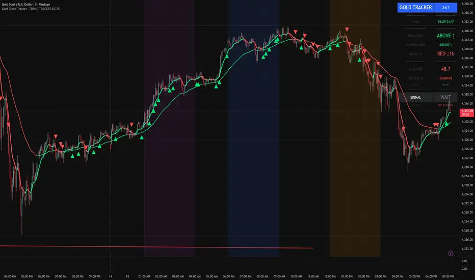
Gold Trend Tracker - TREND TRACKER DG25Gold Trend Tracker - Complete All-In-One Trading System
A professional, institutional-grade trading system specifically optimized for Gold (XAU/USD) that combines multiple technical indicators with session-based filtering and real-time performance tracking. No external indicators required - everything you need is built right in!
🎯 CORE FEATURES
Multi-Layered Confirmation System:
Dynamic EMA trend filter (default 10-period) with color-coded visualization
Optional secondary confirmation EMA (21-period) for stronger validation
3-minute MACD analysis with histogram tracking and direction monitoring
MACD bounce detection for high-probability continuation entries
Built-in Stochastic RSI (K=3, D=3, RSI Length=14, Stochastic Length=14)
Option to connect external Stochastic RSI if preferred
Intelligent Signal Generation:
Clear BUY/SELL triangles plotted directly on price chart
Minimum bars filter to eliminate signal spam and overtrading
Higher timeframe signal overlay (optional) - see 3min signals on 15min chart
Visual Stochastic RSI threshold cross markers (customizable shapes & sizes)
"Show Only First Cross" option to reduce visual clutter
Comprehensive alert system for all signal types
Advanced Session Management:
Pre-configured trading sessions: Asian (1-4am), London (6-9am), NY (12-3pm)
Timezone-aware filtering supporting major financial centers:
Europe/London
America/New_York
America/Chicago
Europe/Paris
Asia/Tokyo
Asia/Dubai
Color-coded session backgrounds (purple/blue/orange)
Individual session toggle switches
24/7 mode for continuous trading (crypto/forex)
Signals only generate during active sessions
Real-Time Performance Tracking:
Live P/L calculation since last signal entry
Customizable lot size for accurate dollar calculations
Pip movement tracking with automatic conversion
Last signal type and duration display
Performance color-coding (green profits, red losses)
Professional Dashboard:
Clean, scalable interface (Small/Medium/Large sizing)
Current time and active session display
Trading status indicator (TRADING/PAUSED/24/7)
Price position relative to Main EMA (ABOVE ↑ / BELOW ↓)
Confirmation EMA status (when enabled)
3-minute MACD color, direction arrow, and bar count
Stochastic RSI value with color-coded status
RSI status: BULLISH/BEARISH/NEUTRAL
Source type indicator (Built-in/External)
Large, clear SIGNAL display: BUY NOW / SELL NOW / WAIT
Performance summary: signal type + price change + dollar value
📊 HOW THE SYSTEM WORKS
BUY Signal Requirements:
✓ Price trading ABOVE main EMA (bullish trend confirmation)
✓ 3-minute MACD crosses above zero OR bounces higher after crossover
✓ Stochastic RSI K-line above bullish threshold (default 50)
✓ Within an active trading session (if session filter enabled)
✓ Confirmation EMA aligned (if secondary EMA enabled)
✓ Minimum bars since last signal met (prevents overtrading)
SELL Signal Requirements:
✓ Price trading BELOW main EMA (bearish trend confirmation)
✓ 3-minute MACD crosses below zero OR bounces lower after crossover
✓ Stochastic RSI K-line below bearish threshold (default 50)
✓ Within an active trading session (if session filter enabled)
✓ Confirmation EMA aligned (if secondary EMA enabled)
✓ Minimum bars since last signal met (prevents overtrading)
Multi-Confirmation Philosophy:
This system requires ALL conditions to align before generating a signal. This drastically reduces false signals and increases win rate by only trading the highest-probability setups where trend, momentum, and volume all confirm direction.
⚙️ BUILT-IN STOCHASTIC RSI
No External Dependencies:
The indicator includes a fully functional Stochastic RSI calculation based on the standard TradingView formula. No need to hunt for compatible indicators or worry about settings mismatches.
Default Settings (Optimized for Gold):
K Smoothing: 3
D Smoothing: 3
RSI Length: 14
Stochastic Length: 14
Bullish Threshold: 50
Bearish Threshold: 50
How It Works:
Calculates RSI on price data
Applies Stochastic formula to RSI values
Smooths result with K-period SMA
Uses K-line (not D-line) for cleaner, faster signals
Compares to your bullish/bearish thresholds
Generates visual cross markers when thresholds breached
Visual Markers:
Multiple shape options: Circle, Diamond, Square, Cross
Four size options: Tiny, Small, Normal, Large
Customizable colors for bullish/bearish crosses
"Show Only First Cross" prevents repetitive markers
Appears below bars (bullish) or above bars (bearish)
Flexibility:
Switch to "External" mode to connect your own Stochastic RSI indicator
Adjust all calculation parameters to match your trading style
Completely disable the filter if you prefer trend + MACD only
🎨 CUSTOMIZATION OPTIONS
Indicators:
Adjust Main EMA length (default 10)
Enable/disable Confirmation EMA (default OFF)
Set Confirmation EMA length (default 21)
Modify MACD parameters (Fast 5, Slow 14, Signal 9)
Enable/disable MACD bounces (default ON)
Set max bounces per trend (1-10, default 2)
Stochastic RSI:
Choose Built-in or External source
Adjust K/D smoothing periods
Modify RSI and Stochastic lengths
Set custom bullish/bearish thresholds
Configure cross marker appearance
Toggle dashboard display
Signals:
Show/hide signal triangles
Set minimum bars between signals (0-50, default 5)
Enable higher timeframe signal overlay
Choose HTF timeframe (e.g., 3min on 15min chart)
Sessions:
Enable/disable session filtering
Select your timezone
Toggle individual sessions (Asian/London/NY)
Customize session start/end hours
Show/hide session background colors
Display:
Choose dashboard size (Small/Medium/Large)
Adjust all visual elements
Customize colors and styling
💡 PRO TRADING TIPS
Session Optimization:
London Session (6-9am): Highest volatility, best for breakout trades
NY Session (12-3pm): Strong trends, ideal for momentum continuation
Avoid Asian Session (1-4am): Lower liquidity, choppier price action
Overlap Period (12-3pm London time): Peak volume, clearest signals
Signal Filtering:
Set 3-5 bars minimum between signals to avoid overtrading
Higher values (7-10 bars) for more conservative, swing-style entries
Lower values (1-3 bars) for aggressive scalping during high volatility
Confirmation EMA Usage:
Enable in choppy/ranging markets for extra validation
Disable during strong trending conditions (adds lag)
Set to 21 for short-term trends, 50 for medium-term
MACD Bounce Strategy:
Bounces occur when MACD histogram changes direction after crossover
Max 2 bounces = optimal (catches first continuation)
Max 1 bounce = conservative (only initial momentum shift)
Max 3-5 bounces = aggressive (catches multiple waves)
Stochastic RSI Thresholds:
50/50 = Balanced (default, works for most conditions)
30/70 = Conservative (fewer but stronger signals)
60/40 = Aggressive (more signals, requires tighter stops)
Adjust based on current market volatility
Risk Management:
Use the performance tracker to trail stops
Exit when dashboard shows opposite signal forming
Monitor MACD direction arrows for momentum shifts
Set profit targets based on average session ranges
🚀 QUICK START GUIDE
For Beginners:
Add indicator to 3-minute Gold (XAU/USD) chart
Leave all default settings (everything is pre-optimized)
Enable London session (6-9am) and NY session (12-3pm)
Set your timezone to your location
Wait for BUY/SELL triangle + "BUY NOW"/"SELL NOW" on dashboard
Enter trade when ALL conditions align
Exit on opposite signal or dashboard status change
For Advanced Traders:
Optimize EMA lengths for your preferred timeframe
Adjust Stochastic RSI thresholds based on backtesting
Fine-tune MACD bounce count for your risk tolerance
Enable Confirmation EMA for extra validation
Use HTF signal overlay for multi-timeframe confluence
Set signal filter to match your trading frequency
Customize session times for your specific market focus
📈 BEST TIMEFRAMES
Primary: 3-minute chart (system is MACD-optimized for 3min)
Alternative: 5-minute, 15-minute (adjust signal filter accordingly)
NOT Recommended: 1-minute (too noisy), 1-hour+ (signals too infrequent)
Chart Setup:
Main Chart: Your preferred timeframe (3min recommended)
MACD: Always references 3-minute data internally
Stochastic RSI: Calculates on current chart timeframe
Session Filter: Works on any timeframe
✅ WHAT MAKES THIS SYSTEM UNIQUE
All-In-One Solution:
✓ No hunting for compatible external indicators
✓ No configuration headaches or version conflicts
✓ One indicator = complete trading system
Session Intelligence:
✓ Only trades during optimal liquidity periods
✓ Automatically pauses during low-volume sessions
✓ Timezone-aware for global traders
Multi-Confirmation:
✓ Trend (EMA) + Momentum (MACD) + Volume (Stochastic RSI)
✓ Drastically reduces false signals
✓ Higher win rate through layered validation
Performance Transparency:
✓ Real-time P/L tracking on every trade
✓ Know your performance immediately
✓ Data-driven decision making
Professional Grade:
✓ Clean, institutional-style dashboard
✓ Customizable for any trading style
✓ Comprehensive alert system
⚠️ IMPORTANT NOTES
This is NOT a "Holy Grail":
No indicator is 100% accurate
Requires proper risk management
Works best during trending conditions
May produce whipsaws in choppy/ranging markets
Risk Disclosure:
Always use stop losses
Never risk more than 1-2% per trade
Past performance doesn't guarantee future results
Practice on demo account first
Optimization:
Default settings are optimized for Gold (XAU/USD)
May require adjustment for other instruments
Backtest on your specific market before live trading
Different session times may work better for your timezone
🔔 ALERTS INCLUDED
BUY Signal Alert
SELL Signal Alert
Stochastic RSI Cross Above Threshold
Stochastic RSI Cross Below Threshold
Alert Setup:
Click "Create Alert" button
Select desired alert condition
Choose notification method (popup/email/SMS/webhook)
Never miss a high-probability setup!
💬 SUPPORT & UPDATES
This indicator is actively maintained and updated based on user feedback. Future updates may include:
Additional timeframe options
More session presets
Enhanced performance analytics
Multi-asset optimization
Tags: Gold Trading, XAU/USD, Trend Following, MACD Strategy, Stochastic RSI, Session Trading, Day Trading, Scalping, London Session, New York Session, EMA System, Multi-Timeframe Analysis, Trading Dashboard, Performance Tracking
EM Levelsstdv levels for you using VIX and VXN for ES and NQ so hopefully it helps you try it out and have fun

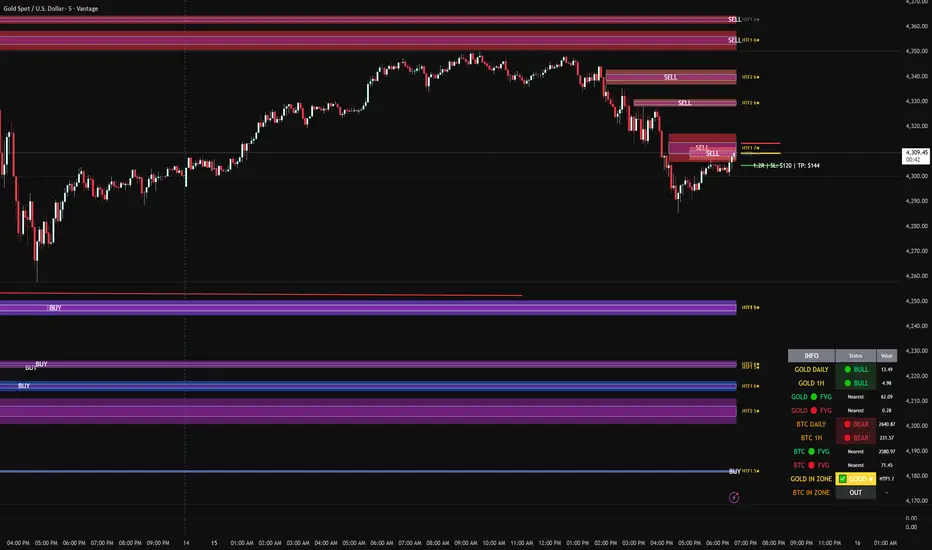
FVG DUAL HTF ALERTS - DG - FVG Dual HTF ALERTS DG - Confluence & Strength
Professional Fair Value Gap (FVG) Trading Indicator with Advanced HTF Analysis
This powerful indicator identifies and tracks Fair Value Gaps across two customizable higher timeframes (HTF), providing traders with precise entry zones, strength ratings, and real-time alerts for high-probability trading setups.
🎯 KEY FEATURES
Dual HTF Analysis
Two independent HTF settings - Analyze FVGs from any timeframe (1min to Daily)
Works on ALL timeframes - View 15min and 60min FVGs on your 1min chart
HTF confluence detection - Automatically highlights when both HTFs align
Customizable colors - Distinct colors for HTF1 and HTF2 zones
Intelligent Strength Scoring (0-10)
Each FVG receives a comprehensive strength rating based on:
Gap size relative to ATR
Volume analysis vs 20-period average
Current timeframe FVG confluence (★ indicator)
Trading session timing (London/NY sessions)
Large gap bonus
HTF confluence bonus
Rating System:
8-10 = 🔥 PREMIUM (Green) - Highest probability setups
5-7 = ✅ GOOD (Yellow) - Quality opportunities
0-4 = ⚠️ WEAK (Gray) - Lower confidence zones
Sweet Spot Inner Boxes
Precision entry zones - 10% inner box (customizable 1-50%)
BUY/SELL labels - Clear directional indicators
Customizable styling - Colors, borders, and text size
Entry optimization - Target the highest probability area within each FVG
Advanced Trading Tools
Automatic Entry/Stop/Target Lines - Up to 3 closest FVGs displayed simultaneously
Risk/Reward calculator - Shows R multiples and dollar values
Customizable position sizing - Micro, mini, or standard lots
Entry offset adjustment - Fine-tune entries ±50 pips from sweet spot center
Smart Fill Detection
HTF candle-based fills - Only checks for fills on HTF candle closes (not every lower TF bar)
Multiple fill methods:
Any Touch - Most sensitive
Midpoint Reached - Balanced
Wick Sweep - Conservative (default)
Body Beyond - Most strict
Touched tracking - Visual feedback when zones are tested
Comprehensive Alert System
8 Individual Alerts:
HTF1: Bullish/Bearish Zone Entry
HTF1: BUY/SELL Sweet Spot Entry
HTF2: Bullish/Bearish Zone Entry
HTF2: BUY/SELL Sweet Spot Entry
4 Combined Alerts:
ANY HTF: Bullish/Bearish Zone Entry
ANY HTF: BUY/SELL Sweet Spot Entry
Plus: Optional alerts for high-strength FVGs (8+)
Information Dashboard
Real-time market context display:
Gold Daily & 1H - Bullish/bearish bias with range in pips
Distance to nearest FVGs - Bull and bear zones
IN ZONE indicator - Shows when price enters sweet spots with strength rating
Optional BTC tracking - Monitor Bitcoin FVGs and bias simultaneously
⚙️ CUSTOMIZATION OPTIONS
Display Settings
Max FVGs to show per type (1-100)
Show only untouched FVGs option
Center line styling (solid/dashed/dotted)
Label visibility and colors
Strength color coding
Trading Parameters
Stop loss (1-100 pips)
Take profit (1-200 pips)
Entry offset adjustment
Lot size (0.01-100)
Dollar value display toggle
Advanced Options
Min strength filter (0-10)
Current TF confluence check
Lookback period (20-200 bars)
Max bars back (1-5000)
Require body close through gap
Test mode: Disable fill removal
💡 IDEAL FOR
Scalpers - 1min/3min charts viewing 5min/15min FVGs
Day Traders - 5min/15min charts viewing 15min/60min FVGs
Swing Traders - 1H/4H charts viewing 4H/Daily FVGs
Gold (XAU/USD) traders - Built-in gold bias indicators
Multi-timeframe analysis - See the bigger picture while trading lower TFs
🎓 HOW TO USE
Add to chart - Works best on 1-5min charts for intraday trading
Set your HTFs - Recommended: 15min + 60min for scalping
Watch for confluence - Green/orange borders indicate HTF alignment
Filter by strength - Focus on 8+ rated zones for best probability
Enter at sweet spots - Wait for price to reach inner boxes
Set alerts - Get notified when price enters high-quality zones
Manage risk - Use provided entry/stop/target lines
📊 BEST PRACTICES
✅ DO:
Focus on 8+ strength FVGs during London/NY sessions
Look for HTF confluence (lime/orange borders)
Wait for sweet spot entries (inner boxes)
Trade in the direction of HTF bias
Use multiple timeframe confirmation
❌ DON'T:
Trade low-strength FVGs (below 5) unless confirmed
Ignore the HTF bias indicators
Chase price - let it come to the zones
Trade without stops
Overtrade - quality over quantity
🔧 TECHNICAL NOTES
Max 500 boxes/lines/labels - Optimized for performance
Lookahead enabled - Accurate HTF data on lower timeframes
No repainting - All signals confirmed on bar close
Compatible with all brokers - Works on any instrument with FVGs
Mobile friendly - Clean display on all devices
📈 PERFORMANCE TIPS
For best results on lower timeframes (1min/3min):
Set "Max Bars Back" to 2000-3000
Set "Max FVGs Per Type" to 20-50
Use "Body Beyond" fill method for longer zone visibility
Enable "Check Current TF FVGs" for additional confluence
🎨 COLOR RECOMMENDATIONS
HTF1 (15min):
Bull: Blue (#2962FF80)
Bear: Red (#f2364580)
HTF2 (60min):
Bull: Purple (#9C27B080)
Bear: Light Red (#FF6B6B80)
Confluence:
Bull: Green (#00FF0060)
Bear: Orange (#FF6B0060)
💬 SUPPORT
Created by DJG9911
For questions, feature requests, or bug reports, please use the TradingView comments section.
Version: 6.0
License: Mozilla Public License 2.0
Last Updated: December 2024
Disclaimer: This indicator is for educational and informational purposes only. Always practice proper risk management and never risk more than you can afford to lose. Past performance does not guarantee future results.
Bullish Structure (PAID) by @Crypto_alphabitTVC:GOLD
This script is for bullish structure........
___________________________________
to confirm the bullish structure , the price has to confirm the second higher low to confirm the uptrend ( ⬜️ The key level ) then the other levels will be automatic calculated with mathematic formula .
This indicator contains some important levels as below ....
__________________________________________________
🟥Stop Loss / lowest point
This level is the lowest point or 0 level & you can consider it as Stop Loss
🟫Strong support(0)
This level is very strong support and the price may not come back to that price after making the key level
⬜️The key Level
This level is the second higher low so the bullish structure confirmed for uptrend
🟪accumulation level(1) , 🟪accumulation level(2) , 🟪accumulation level(3)
The price is slowly moving between the 3 accumulation levels but if the price crossed the 3 levels with momentum , means we are in a very strong uptrend
🟫Strong Support(1) , 🟫Strong Support(2)
Those 2 levels are very strong support and strong resistance in the same time
⬜️Resistance
This level is very important as if the price closed above it so it is high probability that the price will go to the safe Exit
🟩Safe Exit
This is safest exit
🟨Golden Exit
This level is the golden exit if the price reached
🟦Extra Exit(1) , 🟦Extra Exit(2) , 🟦Extra Exit(3)
The price may or may not reach the 3 extra exit levels , it depends on the chart analysis, Gaps and momentum .
🟦Final Exit
This is the final target for that wave
In this indicator you can change some inputs to make it perfect as below ....
__________________________________________________
* Lookback Period for High/Low
* Line Width
* Show/ Hide Price Labels
* Label Size
* Extend Drawing for X Bars
* Swing Sensitivity ( Very important)
*** To confirm the bullish momentum you can add MACD indicator as a helper ***
*** To confirm the targets you can match the targets with Gaps ***
________________________________________________________________
This script is by @Crypto_alphabit

BTC - ALSI: Altcoin Season Index (Dynamic Eras)Title: BTC - ALSI: Altcoin Season Index (Dynamic Eras)
Overview & Philosophy
The Altcoin Season Index (ALSI) is a quantitative tool designed to answer the most critical question in crypto capital rotation: "Is it time to hold Bitcoin, or is it time to take risks on Altcoins?"
Most "Altseason" indicators suffer from Survivor Bias or Obsolescence. They either track a static list of coins that includes "dead" assets from previous cycles (ghosts of 2017), or they break completely when major tokens collapse (like LUNA or FTT).
This indicator solves this by using a Time-Varying Basket. The indicator automatically adjusts its reference list of Top 20 coins based on historical eras. This ensures the index tracks the winners of the moment—capturing the DeFi summer of 2020, the NFT craze of 2021, and the AI/Meme narratives of 2024/2025.
Methodology
The indicator calculates the percentage of the Top 20 Altcoins that are outperforming Bitcoin over a rolling window (Default: 90 Days).
The "Win" Count: For every major Altcoin performing better than BTC, the index adds a point.
Dynamic Eras: The basket of coins changes depending on the date:
2020 Era (DeFi Summer): Tracks the "Blue Chips" of the DeFi revolution like UNI, LINK, DOT, and early movers like VET and FIL.
2021 Era (Layer 1 Wars): Tracks the explosion of alternative smart contract platforms, adding winners like SOL, AVAX, MATIC, and ALGO.
2022 Era (The Survivors): Filters for resilience during the Bear Market, solidifying the status of established assets like SHIB and ATOM.
2023 Era (Infrastructure & Scale): Captures the rise of "Next-Gen" tech leading into the pre-halving year, introducing TON, APT (Aptos), and ARB (Arbitrum).
2024/25 Era (AI & Speed): Tracks the current Super-Cycle leaders, focusing on the AI narrative (TAO, RNDR), High-Performance L1s (SUI), and modern Memes (PEPE).
Chart Analysis & Strategy ( The "Alpha" )
As seen in the chart above, there is a strong correlation between ALSI Peaks and local tops in TOTAL3 (The Crypto Market Cap excluding BTC & ETH).
The Entry (Rotation): When the indicator rises above the neutral 50 line, it signals that capital is beginning to rotate out of Bitcoin and into Altcoins. This has historically been a strong confirmation signal to increase exposure to high-beta assets.
The Exit (Saturation): When the indicator hits 100 (or sustains in the Red Zone > 75), it means every single Altcoin is beating Bitcoin. Historically, this extreme exuberance often marks a local top in the TOTAL3 chart. This is the zone where smart money typically sells into strength, rather than opening new positions.
How to Read the Visuals
🚀 Altcoin Season (Red Zone > 75): Strong Altcoin dominance. The market is "Risk On."
🛡️ Bitcoin Season (Blue Zone < 25): Bitcoin dominance. Alts are bleeding against BTC. Historically, this is a defensive zone to hold BTC or Stablecoins.
Data Dashboard: A status table in the bottom-right corner displays the live Index Value, current Regime, and a System Check to ensure all 20 data feeds are active.
Settings
Lookback Period: Default 90 Days. Lowering this (e.g., to 30) makes the index faster but noisier.
Thresholds: Adjustable zones for Altcoin Season (Default: 75) and Bitcoin Season (Default: 25).
Credits & Attribution
This open-source indicator is built on the shoulders of giants. I acknowledge the original creators of the concept and the pioneers of its implementation on TradingView:
Original Concept: BlockchainCenter.net. - They established the industry standard definition: 75% of the Top 50 coins outperforming Bitcoin over 90 days = Altseason..
TradingView Implementation: Adam_Nguyen - He implemented the "Dynamic Era" logic (updating the coin list annually) on TradingView. Our code structure for the time-based switching is inspired by his methodology. See also his implementation in the chart. ( Altcoin Season Index - Adam) .
Comparison: Why use ALSI | RM?
While inspired by the above, ALSI introduces three key improvements:
Open Source: Unlike other popular TradingView versions (which are closed-source), this script is fully transparent. You can see exactly which coins are triggering the signal.
Sanitized History (Anti-Fragile): Historical Top 20 snapshots are not blindly used. "Dead" coins (like LUNA and FTT) from previous eras are manually filtered out. A raw index would crash during the Terra/FTX collapses, giving a false "Bitcoin Season" signal purely due to bad actors. The curated list preserves the integrity of the market structure signal.
Narrative Relevance: The 2024/25 basket was updated to include TAO (Bittensor) and RNDR, ensuring the index captures the dominant AI narrative, rather than tracking fading assets from the previous cycle.
You can compare the ALSI indicator with other available tradingview indicators in the chart: Different indicators for the same idea are shown in the 3 Pane window below the BTC and Total3 chart, whereas ALSI is the top pane indicator.
Important Note on Coin Selection Baskets are highly curated: Dead/irrelevant coins (FTT, LUNA, BSV) are excluded for clean signals. This prevents historical breaks and ensures Era T5 captures current narratives (AI, Memes) via TAO/RNDR. See above. Users are free to adjust the source code to test their own baskets.
Disclaimer
This script is for research and educational purposes only. Past correlations between ALSI and TOTAL3 do not guarantee future results. Market regimes can change, and "Altseasons" can be cut short by macro events.
Tags
bitcoin, btc, altseason, dominance, total3, rotation, cycle, index, alsi, Rob Maths

Bollinger Bands Forecast with Signals (Zeiierman)█ Overview
Bollinger Bands Forecast with Signals (Zeiierman) extends classic Bollinger Bands into a forward-looking framework. Instead of only showing where volatility has been, it projects where the basis (midline) and band width are likely to drift next, based on recent trend and volatility behavior.
The projection is built from the measured slopes of the Bollinger basis, the standard deviation (or ATR, depending on the mode), and a volatility “breathing” component. On top of that, the script includes an optional projected price path that can be blended with a deterministic random walk, plus rejection signals to highlight failed band breaks.
█ How It Works
⚪ Bollinger Core
The script first computes standard Bollinger Bands using the selected Source, Length, and Multiplier:
Basis = SMA(Source, Length)
Band width = Multiplier × StDev(Source, Length)
Upper/Lower = Basis ± Width
This remains the “live” (non-forecast) structure on the chart.
⚪ Trend & Volatility Slope Estimation
To project forward, the indicator measures directional drift and volatility drift using linear regression differences:
Basis slope from the Bollinger basis
StDev slope from the Bollinger deviation
ATR slope for ATR-based projection mode
These slopes drive the forecast bands forward, reflecting the market’s recent directional and volatility regime.
⚪ Projection Engine (Forecast Bands)
At the last bar, the indicator draws projected basis, upper, and lower lines out to Forecast Bars. The projected basis can be:
Trend (straight linear projection)
Curved (ease-in/out transition toward projected endpoints)
Smoothed (extra smoothing on projected basis/width)
⚪ Price Path Projection + Optional Random Walk
In addition to projecting the bands, the script can draw a price forecast path made of a small number of zigzag swings.
Each swing targets a point offset from the projected basis by a multiple of the projected half-width (“width units”).
Decay gradually reduces swing size as the forecast deepens.
The Optional Random Walk Blend adds a deterministic drift component to the zigzag path. It’s not true randomness; it’s a stable pseudo-random sequence, so the drawing doesn’t jump around on refresh, while still adding “natural” variation.
⚪ Rejection Signals
Signals are based on failed attempts to break a band:
Bear Signal (Down): price tries to push above the upper band, then falls back inside, while still closing above the basis.
Bull Signal (Up): price tries to push below the lower band, then returns back inside, while still closing below the basis.
█ How to Use
⚪ Forward Support/Resistance Corridors
Treat the projected upper/lower bands as a future volatility envelope, not a guarantee:
The upper projection ≈ is likely a resistance level if the regime persists
The lower projection ≈ is likely a support level if the regime persists
Best used for trade planning, targets, and “where price could travel” under similar conditions.
⚪ Regime Read: Trend + Volatility
The projection shape is informative:
Rising basis + expanding width → trend with increasing volatility (needs wider stops / more caution)
Flat basis + compressing width → contraction regime (often precedes expansion)
⚪ Signals for Mean-Reversion / Failed Breakouts
The rejection markers are useful for fade-style setups:
A Down signal near/after upper-band failure can imply rotation back toward the basis.
An Up signal near/after lower-band failure can imply snap-back toward the basis.
With MA filtering enabled, signals are constrained to align with the broader bias, helping reduce chop-driven noise.
█ Related Publications
Donchian Predictive Channel (Zeiierman)
█ Settings
⚪ Bollinger Band
Controls the live Bollinger Bands on the chart.
Source – Price used for calculations.
Length – Lookback period; higher = smoother, lower = more reactive.
Multiplier – Bandwidth; higher = wider bands, lower = tighter bands.
⚪ Forecast
Controls the forward projection of the Bollinger Bands.
Forecast Bars – How far into the future the bands are projected.
Trend Length – Lookback used to estimate trend and volatility slopes.
Forecast Band Mode – Defines projection behavior (linear, curved, breathing, ATR-based, or smoothed).
⚪ Price Forecast
Controls the projected price path inside the bands.
ZigZag Swings – Number of projected oscillations.
Amplitude – Distance from basis, measured in bandwidth units.
Decay – Shrinks swings further into the forecast.
⚪ Random-Walk
Adds controlled randomness to the price path.
Enable – Toggle random-walk influence.
Blend – Strength of randomness vs. zigzag.
Step Size – Size of random steps (band-width units).
Decay – Reduces randomness as the forecast deepens.
Seed – Changes the (stable) random sequence.
⚪ Signals
Controls rejection/mean-reversion signals.
Show Signals – Enable/disable signal markers.
MA Filter (Type/Length) – Filters signals by trend direction.
-----------------
Disclaimer
The content provided in my scripts, indicators, ideas, algorithms, and systems is for educational and informational purposes only. It does not constitute financial advice, investment recommendations, or a solicitation to buy or sell any financial instruments. I will not accept liability for any loss or damage, including without limitation any loss of profit, which may arise directly or indirectly from the use of or reliance on such information.
All investments involve risk, and the past performance of a security, industry, sector, market, financial product, trading strategy, backtest, or individual's trading does not guarantee future results or returns. Investors are fully responsible for any investment decisions they make. Such decisions should be based solely on an evaluation of their financial circumstances, investment objectives, risk tolerance, and liquidity needs.
