Stochastic Pop and Drop by Jake Bernstein v1 [Bitduke]I found a simple strategy by Jake Bernstein, modified it a little and created a strategy with Risk Management System (SL+TP); After that I test it on the different cryptocurrency pairs.
About the Indicator
Basically it's the strategy of 2 indicators: Stochastic Oscillator to define the bias and Average Directional Index to confirm it.
One again, It uses Stochastic Oscillator to define the trading bias. In particular, the trading bias was deemed bullish when the weekly 14-period Stochastic Oscillator was above some default value (in him paper - 50) and rising and vice versa.
Once the trading bias is established, Steckler used the Average Directional Index (ADX) to define a slowdown in the trend. ADX measures the strength of the trend and a move below 20 signals a weak trend.
Modifications
I didn't implement Average Directional Index (ADX) and test just different sources for data, oscillator periods and different levels in relation to the crypto market.
So, it shows good results with two tight thresholds at 55 and 45 level.
The bar chart below the defining the bullish and bearish periods (green and red) and gives a signal to enter the trade (purple bars).
Backtesting
Backtested on XBTUSD , BTCPERP (FTX) pairs. You may notice it shows good results on 3h timeframe.
Relatively low drawdown
~ 10% (from 2019 to date) FTX
~ 22% (4 years from 2016) Bitmex
I backtested on the different altcoin pairs as well, but the results were just not good.
Relatively good results were shown by some index pairs from the FTX exchange ( FTX:SHITPERP ), but I think there is a few data for backtesting to be asure in them.
Bitmex 3h (2017 - 2020) :
i.imgur.com
FTX 3h (2019 - 2020):
i.imgur.com
Possible Improvements
- Regarding trading algorithm it would be good to check with strategy with ADX somehow. Maybe for the better entries
- As for Risk Management system, it can be improved by adding trailing stop to the strategy.
Link: school.stockcharts.com
In den Scripts nach "backtest" suchen

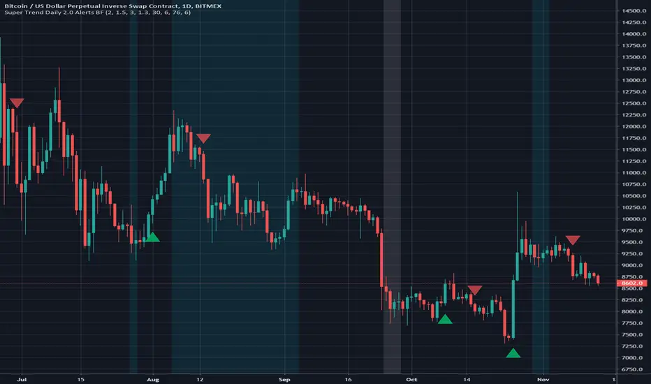
Super Trend Daily 2.0 Alerts BFThis is an alerts script for my Super Trend 2.0 indicator . It is intended as a companion script so you can backtest using the Strategy script and generate alerts using this Study script.
This Study script has the same default settings as the Strategy script and its only purpose is to provide alerts for the long and short signals the Strategy generates. Obviously, if you want to generate alerts based on a Strategy backtest, please ensure the settings are the same in the Study as in the Strategy.
For illustration, I have plotted arrows on the chart for long and short signals, and also colored the background to show when the rate of change function determines a choppy/sideways market.
ALERTS
There are 2 alerts set up:
Long Entry
Short Entry
ILLUSTRATION
Green arrow = Long Entry
Red arrow = Short Entry
White background = No short trades
Aqua background = No long trades
EXAMPLE USE CASE
1. Open a Bitcoin/USD chart on 1D timeframe.
2. Open this script and the Super Trend 2.0 indicator script.
3. Backtest with the Strategy Backtester and change the settings if you like until you get a desirable outcome for your own purposes.
4. Once you are happy with the backtest, change the settings in the Alerts script (this one) so they match the Strategy settings.
5. Set up the alerts according to your preferences.
Advanced ICC Multi-Timeframe 1.0Advanced ICC Multi-Timeframe Trading System
A comprehensive implementation and interpretation of the Indication, Correction, Continuation (ICC) trading methodology made popular by Trades by Sci, enhanced with advanced multi-timeframe analysis and automation features.
⚠️ CRITICAL TRADING WARNINGS:
DO NOT blindly follow BUY/SELL signals from this indicator
This indicator shows potential entry points but YOU must validate each trade
PAPER TRADE EXTENSIVELY before risking real capital
BACKTEST THOROUGHLY on your chosen instruments and timeframes
The ICC methodology requires understanding and discretion - automated signals are guidance only
This tool aids analysis but does not replace proper trade planning, risk management, or trader judgment
⚠️ Important Disclaimers:
This indicator is not endorsed by or affiliated with Trades by Sci
This is an early implementation and interpretation of the ICC methodology
May not work exactly as Trades by Sci executes his trades and entries
Requires further debugging, backtesting, and real-world validation
Completely free to use - no purchase required
I'm just one person obsessed with this method and wanted some better visualization of the chart/entries
About ICC:
The ICC method identifies complete market cycles through three phases: Indication (breakout), Correction (pullback), and Continuation (entry). This indicator automates the identification of these phases and adds powerful features for modern traders.
Key Features:
Multi-Timeframe Capabilities:
Automatic timeframe detection with optimized settings for 5m, 15m, 30m, 1H, 4H, and Daily charts
Higher timeframe overlay to view HTF ICC levels on lower timeframe charts for precise entry timing
Smart defaults that adjust swing length and consolidation detection based on your timeframe
Advanced Phase Tracking:
Complete ICC cycle tracking: Indication, Correction, Consolidation, Continuation, and No Setup phases
Live structure detection shows potential peaks/troughs before full confirmation
Intelligent invalidation logic detects failed setups when market structure reverses
Dynamic phase backgrounds for instant visual confirmation
Three Types of Entry Signals:
Traditional Entries - Price crosses back through the original indication level (strongest signals)
"BUY" (green) / "SELL" (red)
Breakout Entries - Price breaks out of consolidation range in the same direction
"BUY" (green) / "SELL" (red)
Reversal Entries (Optional, can be toggled off) - Price breaks consolidation in opposite direction, indicating failed setup
"⚠ BUY" (yellow) / "⚠ SELL" (orange)
More aggressive, counter-trend signals
Can be disabled for more conservative trading
Professional Features:
Volatility-based support/resistance zones (ATR-adjusted) that adapt to market conditions
Historical zone tracking (0-3 configurable) with visual hierarchy
Comprehensive real-time info table displaying all key metrics
Full alert system for entries, indications, and consolidation detection
Visual distinction between high-confidence trend entries and cautionary reversal entries
📖 USAGE GUIDE
Entry Signal Types:
The indicator provides three types of entry signals with visual distinction:
Strong Entries (High Confidence):
"BUY" (bright green) / "SELL" (bright red)
Includes traditional entries (crossing back through indication level) and breakout entries (breaking consolidation in trend direction)
These are trend continuation or breakout signals with higher probability
Recommended for all traders
Reversal Entries (Caution - Counter-Trend):
"⚠ BUY" (yellow) / "⚠ SELL" (orange)
Triggered when price breaks out of correction/consolidation in the OPPOSITE direction
Indicates a failed setup and potential trend reversal
More aggressive, counter-trend plays
Can be toggled off in settings for more conservative trading
Recommended only for experienced traders or after thorough backtesting
Swing Length Settings:
The swing length determines how many bars on each side are needed to confirm a swing high/low. This is the most important setting for tuning the indicator to your style.
Auto Mode (Recommended for beginners): Toggle "Use Auto Timeframe Settings" ON
5-minute: 30 bars
15-minute: 20 bars
30-minute: 12 bars
1-hour: 7 bars
4-hour: 5 bars
Daily: 3 bars
Manual Mode: Toggle "Use Auto Timeframe Settings" OFF
Lower values (3-7): More aggressive, detects smaller swings
Pros: More signals, faster entries, catches smaller moves
Cons: More noise, more false signals, requires tighter stops
Best for: Scalping, active day trading, volatile markets
Higher values (12-20): More conservative, only major swings
Pros: More reliable signals, fewer false breakouts, clearer structure
Cons: Fewer signals, delayed entries, might miss smaller opportunities
Best for: Swing trading, position trading, trending markets
Default Manual Setting: 7 bars (balanced for 1H charts)
Minimum: 3 bars
Consolidation Bars Setting:
Determines how many bars without new structure are needed before flagging consolidation.
Lower values (3-10): Faster detection, catches brief pauses, more sensitive
Best for: Lower timeframes, volatile markets, avoiding any chop
Higher values (20-40): More reliable, only flags true extended consolidation
Best for: Higher timeframes, trending markets, patient traders
Current defaults scale with timeframe (more bars needed on shorter timeframes)
Historical S/R Zones:
Shows previous support and resistance levels to provide context.
Default: 2 historical zones (shows current + 2 previous)
Range: 0-3 zones
Visual Hierarchy: Older zones are more transparent with dashed borders
Usage: Higher numbers (2-3) show more historical context but can clutter the chart. Start with 2 and adjust based on your preference.
Live Structure Feature (Yellow Warning ⚠):
Provides early warning of potential structure changes before full confirmation.
What it does: Detects potential swing highs/lows after just 2 bars instead of waiting for full swing_length confirmation
Live Peak: Shows when a high is followed by 2 lower closes (potential top forming)
Live Trough: Shows when a low is followed by 2 higher closes (potential bottom forming)
Important: These are UNCONFIRMED - they may be invalidated if price reverses
Use case: Get early awareness of potential reversals while waiting for confirmation
Displayed in: Info table only (no visual markers on chart to reduce clutter)
Only shows: Peaks higher than last swing high, or troughs lower than last swing low (filters out noise)
Higher Timeframe (HTF) Analysis:
View higher timeframe ICC structure while trading on lower timeframes.
How to enable: Toggle "Show Higher Timeframe ICC" ON
Setup: Set "Higher Timeframe" to your reference timeframe
Example: Trading on 15-minute? Set HTF to 240 (4-hour) or 60 (1-hour)
Example: Trading on 5-minute? Set HTF to 60 (1-hour) or 15 (15-minute)
What it shows:
HTF indication levels displayed as dashed lines
Blue = HTF Bullish Indication
Purple = HTF Bearish Indication
HTF phase and levels shown in info table
Trading workflow:
Check HTF phase for overall market direction
Wait for HTF correction phase
Drop to lower timeframe to find precise entries
Enter when lower TF shows continuation in alignment with HTF
Best practice: HTF should be 3-4x your trading timeframe for best results
Reversal Entries Toggle:
Default: ON (shows all signal types)
Toggle OFF for more conservative trading (only trend continuation signals)
Recommended: Backtest with both settings to see which works better for your style
New traders should consider disabling reversal entries initially
Volatility-Based Zones:
When enabled, support/resistance zones automatically adjust their height based on ATR (Average True Range).
More volatile = wider zones
Less volatile = tighter zones
Toggle OFF for fixed-width zones
Community Feedback Welcome:
This is an evolving project and your input is valuable! Please share:
Bug reports and issues you encounter
Feature requests and suggestions for improvement
Results from your backtesting and live trading experience
Feedback on the reversal entry feature (too aggressive? working well?)
Ideas for better aligning with the ICC methodology
Perfect for traders learning or implementing the ICC methodology with the benefit of modern automation, multi-timeframe analysis, and flexible entry signal options.

EMA 12-26-100 Momentum Strategy# Triple EMA Multi-Signal Momentum Strategy
## 📊 Overview
**Triple EMA Multi-Signal** is a comprehensive trend-following momentum strategy designed specifically for cryptocurrency markets. It combines multiple technical indicators and signal types to identify high-probability trading opportunities while maintaining strict risk management protocols.
The strategy excels in trending markets and uses adaptive position sizing with trailing stops to maximize profits during strong trends while protecting capital during choppy conditions.
## 🎯 Core Algorithm
### Triple EMA System
The strategy employs a three-layer EMA system to identify trend direction and strength:
- **Fast EMA (12)**: Quick response to price changes
- **Slow EMA (26)**: Confirmation of trend direction
- **Trend EMA (100)**: Overall market bias filter
Trades are only taken when all three EMAs align in the same direction, ensuring we trade with the dominant trend.
### Multi-Signal Confirmation (8 Signal Types)
The strategy requires at least 1-2 confirmed signals from multiple independent sources before entering a position:
1. **EMA Crossover** - Fast EMA crossing Slow EMA (primary signal)
2. **MACD Cross** - MACD line crossing signal line (momentum confirmation)
3. **RSI Reversal** - RSI bouncing from oversold/overbought zones
4. **Price Action** - Strong bullish/bearish candles (>60% of range)
5. **Volume Spike** - Above-average volume confirmation
6. **Breakout** - Price breaking 20-period high/low with volume
7. **Pullback to EMA** - Trend continuation after healthy retracement
8. **Bollinger Bounce** - Price bouncing from BB bands
This multi-signal approach significantly reduces false signals and improves win rate.
## 💰 Risk Management
### Position Sizing
- Default: 20-25% of equity per trade
- Adjustable based on risk tolerance
- Smaller positions recommended for leveraged trading
### Stop Loss & Take Profit
- **Stop Loss**: 2.0% (tight control of risk)
- **Take Profit**: 5.5% (2.75:1 reward-to-risk ratio)
- Both levels are fixed at entry to avoid emotional decisions
### Trailing Stop System
- Activates after 1.8% profit
- Trails at 1.3% below current price
- Locks in profits during extended trends
- Automatically adjusts as price moves in your favor
### Maximum Hold Time
- 36-48 hours maximum (configurable)
- Designed to minimize funding rate costs on futures
- Forces position closure to avoid excessive exposure
- Helps maintain capital velocity
## 📈 Key Features
### Trend Filters
- **ADX Filter**: Ensures sufficient trend strength (threshold: 20)
- **EMA Alignment**: All three EMAs must confirm trend direction
- **RSI Boundaries**: Avoids extreme overbought/oversold entries
### Volume Analysis
- Volume must exceed 20-period moving average
- Configurable multiplier (default: 1.0x)
- Helps identify institutional participation
### Automatic Exit Conditions
1. Take Profit target reached
2. Stop Loss triggered
3. Trailing stop activated
4. Trend reversal (EMA cross in opposite direction)
5. Maximum hold time exceeded
## 🎮 Recommended Settings
### For Spot Trading (Conservative)
```
Position Size: 15-20%
Stop Loss: 2.5%
Take Profit: 6.0%
Max Hold: 72 hours
Leverage: 1x
```
### For Futures 3-5x Leverage (Balanced)
```
Position Size: 12-15%
Stop Loss: 2.0%
Take Profit: 5.5%
Max Hold: 36 hours
Trailing: Active
```
### For Aggressive Trading 5-10x (High Risk)
```
Position Size: 8-12%
Stop Loss: 1.5%
Take Profit: 4.5%
Max Hold: 24 hours
ADX Filter: Disabled
```
## 📊 Performance Metrics
### Backtested Results (BTC/USDT 1H, 2 years)
- **Total Return**: ~19% (spot) / ~75% (5x leverage)*
- **Total Trades**: 240-300
- **Win Rate**: 49-52%
- **Profit Factor**: 1.25-1.50
- **Max Drawdown**: ~18-22%
- **Average Trade**: 0.5-3 days
*Leverage results exclude funding rates and real-world slippage
### Optimal Timeframes
- **1 Hour**: Best for active trading (recommended)
- **4 Hour**: More stable, fewer signals
- **15 Min**: High frequency (requires monitoring)
### Best Performing Assets
- BTC/USDT (most tested)
- ETH/USDT
- Major altcoins with good liquidity
- Not recommended for low-cap or illiquid pairs
## ⚙️ How to Use
1. **Add to Chart**: Apply strategy to 1H BTC/USDT chart
2. **Adjust Settings**: Configure risk parameters based on your preference
3. **Review Signals**: Green = Long, Red = Short, labels show signal count
4. **Monitor Performance**: Check strategy tester for detailed statistics
5. **Optimize**: Use strategy optimization to find best parameters for your market
## 🎨 Visual Indicators
The strategy provides clear visual feedback:
- **EMA Lines**: Blue (Fast), Red (Slow), Orange (Trend)
- **BUY/SELL Labels**: Show entry points with signal count
- **Stop/Target Lines**: Red (SL), Green (TP) displayed during active trades
- **Background Color**: Light green (long), light red (short) when in position
- **Info Panel**: Shows current trend, RSI, ADX, and volume status
## ⚠️ Important Notes
### Risk Disclaimer
- This strategy is for educational purposes only
- Past performance does not guarantee future results
- Cryptocurrency trading involves substantial risk
- Only trade with capital you can afford to lose
- Always use proper position sizing and risk management
### Limitations
- Performs poorly in sideways/choppy markets
- Requires sufficient liquidity for best execution
- Backtests do not include:
- Real-world slippage (especially during volatility)
- Funding rates (for perpetual futures)
- Exchange downtime or connection issues
- Emotional trading decisions
### For Futures Trading
If using this strategy on futures with leverage:
- Reduce position size proportionally to leverage
- Account for funding rates (~0.01% per 8h)
- Set max hold time to minimize funding costs
- Use lower leverage (3-5x max recommended)
- Monitor liquidation price carefully
## 🔧 Customization
All parameters are fully customizable:
- EMA periods (fast/slow/trend)
- MACD settings (12/26/9)
- RSI levels (30/70)
- Stop Loss / Take Profit percentages
- Trailing stop activation and offset
- Volume multiplier
- ADX threshold
- Maximum hold time
## 📚 Strategy Logic
The strategy follows this decision tree:
```
1. Check Trend Direction (EMA alignment)
↓
2. Scan for Entry Signals (8 types)
↓
3. Confirm with Filters (ADX, Volume, RSI)
↓
4. Enter Position with Fixed SL/TP
↓
5. Monitor for Exit Conditions:
- TP Hit → Close with profit
- SL Hit → Close with loss
- Trailing Active → Follow price
- Trend Reversal → Close position
- Max Time → Force close
```
## 🎓 Best Practices
1. **Start Conservative**: Use smaller position sizes initially
2. **Track Performance**: Monitor actual vs backtested results
3. **Optimize Regularly**: Market conditions change, adapt parameters
4. **Combine with Analysis**: Don't rely solely on automated signals
5. **Manage Emotions**: Stick to the system, avoid manual overrides
6. **Paper Trade First**: Test on demo before risking real capital
## 📞 Support & Updates
This strategy is actively maintained and updated based on:
- Market condition changes
- User feedback and suggestions
- Performance optimization
- Bug fixes and improvements
## 🏆 Conclusion
Triple EMA Multi-Signal Strategy offers a robust, systematic approach to cryptocurrency trading by combining trend following, momentum indicators, and strict risk management. Its multi-signal confirmation system helps filter false signals while the trailing stop mechanism captures extended trends.
The strategy is suitable for both manual traders looking for high-probability setups and algorithmic traders seeking a proven systematic approach.
**Remember**: No strategy wins 100% of the time. Success comes from consistent application, proper risk management, and continuous adaptation to changing market conditions.
---
*Version: 1.0*
*Last Updated: November 2025*
*Tested on: BTC/USDT, ETH/USDT (1H, 4H timeframes)*
*Recommended Capital: $5,000+ for optimal position sizing*

Volatility-Targeted Momentum Portfolio [BackQuant]Volatility-Targeted Momentum Portfolio
A complete momentum portfolio engine that ranks assets, targets a user-defined volatility, builds long, short, or delta-neutral books, and reports performance with metrics, attribution, Monte Carlo scenarios, allocation pie, and efficiency scatter plots. This description explains the theory and the mechanics so you can configure, validate, and deploy it with intent.
Table of contents
What the script does at a glance
Momentum, what it is, how to know if it is present
Volatility targeting, why and how it is done here
Portfolio construction modes: Long Only, Short Only, Delta Neutral
Regime filter and when the strategy goes to cash
Transaction cost modelling in this script
Backtest metrics and definitions
Performance attribution chart
Monte Carlo simulation
Scatter plot analysis modes
Asset allocation pie chart
Inputs, presets, and deployment checklist
Suggested workflow
1) What the script does at a glance
Pulls a list of up to 15 tickers, computes a simple momentum score on each over a configurable lookback, then volatility-scales their bar-to-bar return stream to a target annualized volatility.
Ranks assets by raw momentum, selects the top 3 and bottom 3, builds positions according to the chosen mode, and gates exposure with a fast regime filter.
Accumulates a portfolio equity curve with risk and performance metrics, optional benchmark buy-and-hold for comparison, and a full alert suite.
Adds visual diagnostics: performance attribution bars, Monte Carlo forward paths, an allocation pie, and scatter plots for risk-return and factor views.
2) Momentum: definition, detection, and validation
Momentum is the tendency of assets that have performed well to continue to perform well, and of underperformers to continue underperforming, over a specific horizon. You operationalize it by selecting a horizon, defining a signal, ranking assets, and trading the leaders versus laggards subject to risk constraints.
Signal choices . Common signals include cumulative return over a lookback window, regression slope on log-price, or normalized rate-of-change. This script uses cumulative return over lookback bars for ranking (variable cr = price/price - 1). It keeps the ranking simple and lets volatility targeting handle risk normalization.
How to know momentum is present .
Leaders and laggards persist across adjacent windows rather than flipping every bar.
Spread between average momentum of leaders and laggards is materially positive in sample.
Cross-sectional dispersion is non-trivial. If everything is flat or highly correlated with no separation, momentum selection will be weak.
Your validation should include a diagnostic that measures whether returns are explained by a momentum regression on the timeseries.
Recommended diagnostic tool . Before running any momentum portfolio, verify that a timeseries exhibits stable directional drift. Use this indicator as a pre-check: It fits a regression to price, exposes slope and goodness-of-fit style context, and helps confirm if there is usable momentum before you force a ranking into a flat regime.
3) Volatility targeting: purpose and implementation here
Purpose . Volatility targeting seeks a more stable risk footprint. High-vol assets get sized down, low-vol assets get sized up, so each contributes more evenly to total risk.
Computation in this script (per asset, rolling):
Return series ret = log(price/price ).
Annualized volatility estimate vol = stdev(ret, lookback) * sqrt(tradingdays).
Leverage multiplier volMult = clamp(targetVol / vol, 0.1, 5.0).
This caps sizing so extremely low-vol assets don’t explode weight and extremely high-vol assets don’t go to zero.
Scaled return stream sr = ret * volMult. This is the per-bar, risk-adjusted building block used in the portfolio combinations.
Interpretation . You are not levering your account on the exchange, you are rescaling the contribution each asset’s daily move has on the modeled equity. In live trading you would reflect this with position sizing or notional exposure.
4) Portfolio construction modes
Cross-sectional ranking . Assets are sorted by cr over the chosen lookback. Top and bottom indices are extracted without ties.
Long Only . Averages the volatility-scaled returns of the top 3 assets: avgRet = mean(sr_top1, sr_top2, sr_top3). Position table shows per-asset leverages and weights proportional to their current volMult.
Short Only . Averages the negative of the volatility-scaled returns of the bottom 3: avgRet = mean(-sr_bot1, -sr_bot2, -sr_bot3). Position table shows short legs.
Delta Neutral . Long the top 3 and short the bottom 3 in equal book sizes. Each side is sized to 50 percent notional internally, with weights within each side proportional to volMult. The return stream mixes the two sides: avgRet = mean(sr_top1,sr_top2,sr_top3, -sr_bot1,-sr_bot2,-sr_bot3).
Notes .
The selection metric is raw momentum, the execution stream is volatility-scaled returns. This separation is deliberate. It avoids letting volatility dominate ranking while still enforcing risk parity at the return contribution stage.
If everything rallies together and dispersion collapses, Long Only may behave like a single beta. Delta Neutral is designed to extract cross-sectional momentum with low net beta.
5) Regime filter
A fast EMA(12) vs EMA(21) filter gates exposure.
Long Only active when EMA12 > EMA21. Otherwise the book is set to cash.
Short Only active when EMA12 < EMA21. Otherwise cash.
Delta Neutral is always active.
This prevents taking long momentum entries during obvious local downtrends and vice versa for shorts. When the filter is false, equity is held flat for that bar.
6) Transaction cost modelling
There are two cost touchpoints in the script.
Per-bar drag . When the regime filter is active, the per-bar return is reduced by fee_rate * avgRet inside netRet = avgRet - (fee_rate * avgRet). This models proportional friction relative to traded impact on that bar.
Turnover-linked fee . The script tracks changes in membership of the top and bottom baskets (top1..top3, bot1..bot3). The intent is to charge fees when composition changes. The template counts changes and scales a fee by change count divided by 6 for the six slots.
Use case: increase fee_rate to reflect taker fees and slippage if you rebalance every bar or trade illiquid assets. Reduce it if you rebalance less often or use maker orders.
Practical advice .
If you rebalance daily, start with 5–20 bps round-trip per switch on liquid futures and adjust per venue.
For crypto perp microcaps, stress higher cost assumptions and add slippage buffers.
If you only rotate on lookback boundaries or at signals, use alert-driven rebalances and lower per-bar drag.
7) Backtest metrics and definitions
The script computes a standard set of portfolio statistics once the start date is reached.
Net Profit percent over the full test.
Max Drawdown percent, tracked from running peaks.
Annualized Mean and Stdev using the chosen trading day count.
Variance is the square of annualized stdev.
Sharpe uses daily mean adjusted by risk-free rate and annualized.
Sortino uses downside stdev only.
Omega ratio of sum of gains to sum of losses.
Gain-to-Pain total gains divided by total losses absolute.
CAGR compounded annual growth from start date to now.
Alpha, Beta versus a user-selected benchmark. Beta from covariance of daily returns, Alpha from CAPM.
Skewness of daily returns.
VaR 95 linear-interpolated 5th percentile of daily returns.
CVaR average of the worst 5 percent of daily returns.
Benchmark Buy-and-Hold equity path for comparison.
8) Performance attribution
Cumulative contribution per asset, adjusted for whether it was held long or short and for its volatility multiplier, aggregated across the backtest. You can filter to winners only or show both sides. The panel is sorted by contribution and includes percent labels.
9) Monte Carlo simulation
The panel draws forward equity paths from either a Normal model parameterized by recent mean and stdev, or non-parametric bootstrap of recent daily returns. You control the sample length, number of simulations, forecast horizon, visibility of individual paths, confidence bands, and a reproducible seed.
Normal uses Box-Muller with your seed. Good for quick, smooth envelopes.
Bootstrap resamples realized returns, preserving fat tails and volatility clustering better than a Gaussian assumption.
Bands show 10th, 25th, 75th, 90th percentiles and the path mean.
10) Scatter plot analysis
Four point-cloud modes, each plotting all assets and a star for the current portfolio position, with quadrant guides and labels.
Risk-Return Efficiency . X is risk proxy from leverage, Y is expected return from annualized momentum. The star shows the current book’s composite.
Momentum vs Volatility . Visualizes whether leaders are also high vol, a cue for turnover and cost expectations.
Beta vs Alpha . X is a beta proxy, Y is risk-adjusted excess return proxy. Useful to see if leaders are just beta.
Leverage vs Momentum . X is volMult, Y is momentum. Shows how volatility targeting is redistributing risk.
11) Asset allocation pie chart
Builds a wheel of current allocations.
Long Only, weights are proportional to each long asset’s current volMult and sum to 100 percent.
Short Only, weights show the short book as positive slices that sum to 100 percent.
Delta Neutral, 50 percent long and 50 percent short books, each side leverage-proportional.
Labels can show asset, percent, and current leverage.
12) Inputs and quick presets
Core
Portfolio Strategy . Long Only, Short Only, Delta Neutral.
Initial Capital . For equity scaling in the panel.
Trading Days/Year . 252 for stocks, 365 for crypto.
Target Volatility . Annualized, drives volMult.
Transaction Fees . Per-bar drag and composition change penalty, see the modelling notes above.
Momentum Lookback . Ranking horizon. Shorter is more reactive, longer is steadier.
Start Date . Ensure every symbol has data back to this date to avoid bias.
Benchmark . Used for alpha, beta, and B&H line.
Diagnostics
Metrics, Equity, B&H, Curve labels, Daily return line, Rolling drawdown fill.
Attribution panel. Toggle winners only to focus on what matters.
Monte Carlo mode with Normal or Bootstrap and confidence bands.
Scatter plot type and styling, labels, and portfolio star.
Pie chart and labels for current allocation.
Presets
Crypto Daily, Long Only . Lookback 25, Target Vol 50 percent, Fees 10 bps, Regime filter on, Metrics and Drawdown on. Monte Carlo Bootstrap with Recent 200 bars for bands.
Crypto Daily, Delta Neutral . Lookback 25, Target Vol 50 percent, Fees 15–25 bps, Regime filter always active for this mode. Use Scatter Risk-Return to monitor efficiency and keep the star near upper left quadrants without drifting rightward.
Equities Daily, Long Only . Lookback 60–120, Target Vol 15–20 percent, Fees 5–10 bps, Regime filter on. Use Benchmark SPX and watch Alpha and Beta to keep the book from becoming index beta.
13) Suggested workflow
Universe sanity check . Pick liquid tickers with stable data. Thin assets distort vol estimates and fees.
Check momentum existence . Run on your timeframe. If slope and fit are weak, widen lookback or avoid that asset or timeframe.
Set risk budget . Choose a target volatility that matches your drawdown tolerance. Higher target increases turnover and cost sensitivity.
Pick mode . Long Only for bull regimes, Short Only for sustained downtrends, Delta Neutral for cross-sectional harvesting when index direction is unclear.
Tune lookback . If leaders rotate too often, lengthen it. If entries lag, shorten it.
Validate cost assumptions . Increase fee_rate and stress Monte Carlo. If the edge vanishes with modest friction, refine selection or lengthen rebalance cadence.
Run attribution . Confirm the strategy’s winners align with intuition and not one unstable outlier.
Use alerts . Enable position change, drawdown, volatility breach, regime, momentum shift, and crash alerts to supervise live runs.
Important implementation details mapped to code
Momentum measure . cr = price / price - 1 per symbol for ranking. Simplicity helps avoid overfitting.
Volatility targeting . vol = stdev(log returns, lookback) * sqrt(tradingdays), volMult = clamp(targetVol / vol, 0.1, 5), sr = ret * volMult.
Selection . Extract indices for top1..top3 and bot1..bot3. The arrays rets, scRets, lev_vals, and ticks_arr track momentum, scaled returns, leverage multipliers, and display tickers respectively.
Regime filter . EMA12 vs EMA21 switch determines if the strategy takes risk for Long or Short modes. Delta Neutral ignores the gate.
Equity update . Equity multiplies by 1 + netRet only when the regime was active in the prior bar. Buy-and-hold benchmark is computed separately for comparison.
Tables . Position tables show current top or bottom assets with leverage and weights. Metric table prints all risk and performance figures.
Visualization panels . Attribution, Monte Carlo, scatter, and pie use the last bars to draw overlays that update as the backtest proceeds.
Final notes
Momentum is a portfolio effect. The edge comes from cross-sectional dispersion, adequate risk normalization, and disciplined turnover control, not from a single best asset call.
Volatility targeting stabilizes path but does not fix selection. Use the momentum regression link above to confirm structure exists before you size into it.
Always test higher lag costs and slippage, then recheck metrics, attribution, and Monte Carlo envelopes. If the edge persists under stress, you have something robust.

Grand Master's Candlestick Dominance (ATR Enhanced)### Grand Master's Candlestick Dominance (ATR Enhanced)
**Overview**
Unleash the ancient wisdom of Japanese candlestick charting with a modern twist! This comprehensive Pine Script v5 strategy and indicator scans for over 75 classic and advanced candlestick patterns (bullish, bearish, and neutral), assigning dynamic strength scores (1-10) to each for precise signal filtering. Enhanced with Average True Range (ATR) for volatility-aware body size validation, it dominates the markets by combining timeless pattern recognition with robust confirmation layers. Whether used as a backtestable strategy or visual indicator, it empowers traders to spot high-probability reversals, continuations, and indecision setups with surgical accuracy.
Inspired by Steve Nison's *Japanese Candlestick Charting Techniques*, this tool elevates pattern analysis beyond basics—think Hammers, Engulfing patterns, Morning Stars, and rare gems like Abandoned Baby or Concealing Baby Swallow—all consolidated into intelligent arrays for real-time averaging and prioritization.
**Key Features**
- **Extensive Pattern Library**:
- **Bullish (25+ patterns)**: Hammer (8.0), Bullish Engulfing (10.0), Morning Star (7.0), Three White Soldiers (9.0), Dragonfly Doji (8.0), and more (e.g., Rising Three, Unique Three River Bottom).
- **Bearish (25+ patterns)**: Hanging Man (8.0), Bearish Engulfing (10.0), Evening Star (7.0), Three Black Crows (9.0), Gravestone Doji (8.0), and exotics like Upside Gap Two Crows or Stalled Pattern.
- **Neutral/Indecision (34+ patterns)**: Doji variants (Long-Legged, Four Price), Spinning Tops, Harami Crosses, and multi-bar setups like Upside Tasuki Gap or Advancing Block.
Each pattern includes duration tracking (1-5 bars) and ATR-adjusted body/shadow criteria for relevance in volatile conditions.
- **Smart Confirmation Filters** (All Toggleable):
- **Trend Alignment**: 20-period SMA (customizable) ensures entries align with the prevailing trend; optional higher timeframe (e.g., Daily) MA crossover for multi-timeframe confluence.
- **Support/Resistance (S/R)**: Pivot-based levels with 0.01% tolerance to confirm bounces or breaks.
- **Volume Surge**: 20-period volume MA with 1.5x spike multiplier to validate momentum.
- **ATR Body Sizing**: Filters small bodies (<0.3x ATR) and long bodies (>0.8x ATR) for context-aware pattern reliability.
- **Follow-Through**: Ensures post-pattern confirmation via bullish/bearish closes or closes beyond prior bars.
Minimum average strength (default 7.0) and individual pattern thresholds (5.0) prevent weak signals.
- **Entry & Exit Logic**:
- **Long Entry**: Bullish average strength ≥7.0 (outweighing bearish), uptrend, volume spike, near support, follow-through, and HTF alignment.
- **Short Entry**: Mirror for bearish dominance in downtrends near resistance.
- **Exits**: Bearish/neutral shift, or fixed TP (5%) / SL (2%)—pyramiding disabled, 10% equity sizing.
- Backtest range: Jan 1, 2020 – Dec 31, 2025 (editable). Initial capital: $10,000.
- **Interactive Dashboard** (Top-Right Panel):
Real-time insights including:
- Market phase (e.g., "Bullish Phase (Avg Str: 8.2)"), active pattern (e.g., "BULLISH: Bullish Engulfing (Str: 10.0, Bars: 2)"), and trend status.
- Strength breakdowns (Bull/Bear/Neutral counts & averages).
- Filter status (e.g., "Volume: ✔ Spike", "ATR: Enabled (L:0.8, S:0.3)").
- Backtest stats: Total trades, win rate, streak, and last entry/exit details (price & timestamp).
Toggle mode: Strategy (live trades) or Indicator (signals only).
- **Advanced Alerts** (15+ Toggleable Types):
Set up via TradingView's "Any alert() function call" for bar-close triggers:
- Entry/Exit signals with strength & pattern details.
- Strong patterns (≥2 bullish/bearish), neutral indecision, volume spikes.
- S/R breakouts, HTF reversals, high-confidence singles (≥8.0 strength).
- Conflicting signals, MA crossovers, ATR volatility bursts, multi-bar completions.
Example: "STRONG BULLISH PATTERN detected! Strength: 9.5 | Top Pattern: Three White Soldiers | Trend: Up".
**Customization & Usage Tips**
- **Inputs Groups**: Strategy toggles, confirmations, exits, backtest dates, and 15+ alert switches—all intuitively grouped.
- **Optimization**: Tune min strengths for aggressive (lower) or conservative (higher) trading; enable/disable filters to suit your style (e.g., disable S/R for scalping).
- **Best For**: Forex, stocks, crypto on 1H–Daily charts. Test on historical data to refine TP/SL.
- **Limitations**: No external data installs; relies on built-in TA functions. Patterns are probabilistic—combine with your risk management.
Master the candles like a grandmaster. Deploy on TradingView, backtest relentlessly, and let dominance begin! Questions? Drop a comment.
*Version: 1.0 | Updated: September 2025 | Credits: Built on Pine Script v5 with nods to Nison's timeless techniques.*

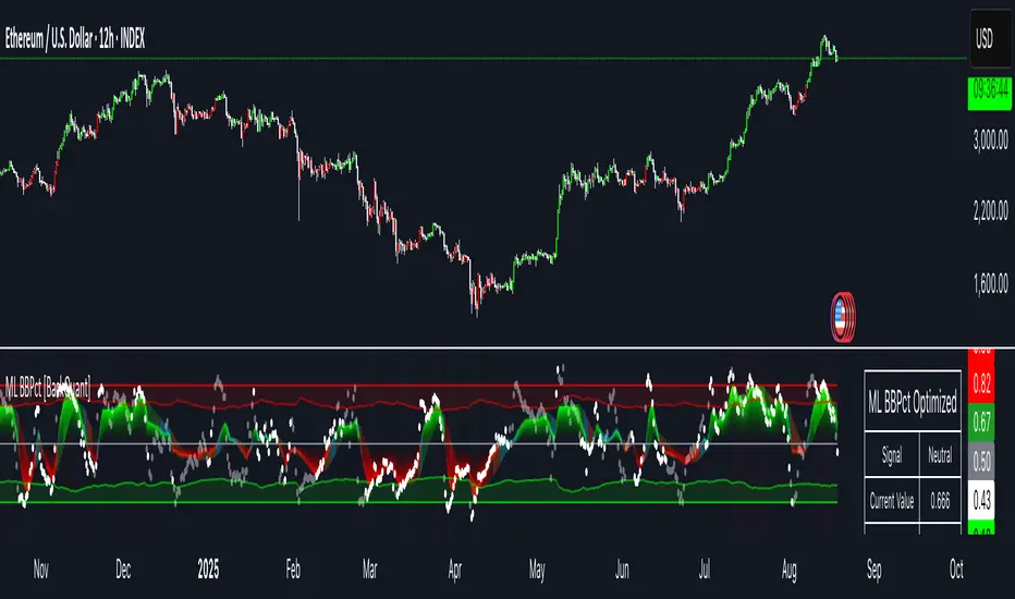
Machine Learning BBPct [BackQuant]Machine Learning BBPct
What this is (in one line)
A Bollinger Band %B oscillator enhanced with a simplified K-Nearest Neighbors (KNN) pattern matcher. The model compares today’s context (volatility, momentum, volume, and position inside the bands) to similar situations in recent history and blends that historical consensus back into the raw %B to reduce noise and improve context awareness. It is informational and diagnostic—designed to describe market state, not to sell a trading system.
Background: %B in plain terms
Bollinger %B measures where price sits inside its dynamic envelope: 0 at the lower band, 1 at the upper band, ~ 0.5 near the basis (the moving average). Readings toward 1 indicate pressure near the envelope’s upper edge (often strength or stretch), while readings toward 0 indicate pressure near the lower edge (often weakness or stretch). Because bands adapt to volatility, %B is naturally comparable across regimes.
Why add (simplified) KNN?
Classic %B is reactive and can be whippy in fast regimes. The simplified KNN layer builds a “nearest-neighbor memory” of recent market states and asks: “When the market looked like this before, where did %B tend to be next bar?” It then blends that estimate with the current %B. Key ideas:
• Feature vector . Each bar is summarized by up to five normalized features:
– %B itself (normalized)
– Band width (volatility proxy)
– Price momentum (ROC)
– Volume momentum (ROC of volume)
– Price position within the bands
• Distance metric . Euclidean distance ranks the most similar recent bars.
• Prediction . Average the neighbors’ prior %B (lagged to avoid lookahead), inverse-weighted by distance.
• Blend . Linearly combine raw %B and KNN-predicted %B with a configurable weight; optional filtering then adapts to confidence.
This remains “simplified” KNN: no training/validation split, no KD-trees, no scaling beyond windowed min-max, and no probabilistic calibration.
How the script is organized (by input groups)
1) BBPct Settings
• Price Source – Which price to evaluate (%B is computed from this).
• Calculation Period – Lookback for SMA basis and standard deviation.
• Multiplier – Standard deviation width (e.g., 2.0).
• Apply Smoothing / Type / Length – Optional smoothing of the %B stream before ML (EMA, RMA, DEMA, TEMA, LINREG, HMA, etc.). Turning this off gives you the raw %B.
2) Thresholds
• Overbought/Oversold – Default 0.8 / 0.2 (inside ).
• Extreme OB/OS – Stricter zones (e.g., 0.95 / 0.05) to flag stretch conditions.
3) KNN Machine Learning
• Enable KNN – Switch between pure %B and hybrid.
• K (neighbors) – How many historical analogs to blend (default 8).
• Historical Period – Size of the search window for neighbors.
• ML Weight – Blend between raw %B and KNN estimate.
• Number of Features – Use 2–5 features; higher counts add context but raise the risk of overfitting in short windows.
4) Filtering
• Method – None, Adaptive, Kalman-style (first-order),
or Hull smoothing.
• Strength – How aggressively to smooth. “Adaptive” uses model confidence to modulate its alpha: higher confidence → stronger reliance on the ML estimate.
5) Performance Tracking
• Win-rate Period – Simple running score of past signal outcomes based on target/stop/time-out logic (informational, not a robust backtest).
• Early Entry Lookback – Horizon for forecasting a potential threshold cross.
• Profit Target / Stop Loss – Used only by the internal win-rate heuristic.
6) Self-Optimization
• Enable Self-Optimization – Lightweight, rolling comparison of a few canned settings (K = 8/14/21 via simple rules on %B extremes).
• Optimization Window & Stability Threshold – Governs how quickly preferred K changes and how sensitive the overfitting alarm is.
• Adaptive Thresholds – Adjust the OB/OS lines with volatility regime (ATR ratio), widening in calm markets and tightening in turbulent ones (bounded 0.7–0.9 and 0.1–0.3).
7) UI Settings
• Show Table / Zones / ML Prediction / Early Signals – Toggle informational overlays.
• Signal Line Width, Candle Painting, Colors – Visual preferences.
Step-by-step logic
A) Compute %B
Basis = SMA(source, len); dev = stdev(source, len) × multiplier; Upper/Lower = Basis ± dev.
%B = (price − Lower) / (Upper − Lower). Optional smoothing yields standardBB .
B) Build the feature vector
All features are min-max normalized over the KNN window so distances are in comparable units. Features include normalized %B, normalized band width, normalized price ROC, normalized volume ROC, and normalized position within bands. You can limit to the first N features (2–5).
C) Find nearest neighbors
For each bar inside the lookback window, compute the Euclidean distance between current features and that bar’s features. Sort by distance, keep the top K .
D) Predict and blend
Use inverse-distance weights (with a strong cap for near-zero distances) to average neighbors’ prior %B (lagged by one bar). This becomes the KNN estimate. Blend it with raw %B via the ML weight. A variance of neighbor %B around the prediction becomes an uncertainty proxy ; combined with a stability score (how long parameters remain unchanged), it forms mlConfidence ∈ . The Adaptive filter optionally transforms that confidence into a smoothing coefficient.
E) Adaptive thresholds
Volatility regime (ATR(14) divided by its 50-bar SMA) nudges OB/OS thresholds wider or narrower within fixed bounds. The aim: comparable extremeness across regimes.
F) Early entry heuristic
A tiny two-step slope/acceleration probe extrapolates finalBB forward a few bars. If it is on track to cross OB/OS soon (and slope/acceleration agree), it flags an EARLY_BUY/SELL candidate with an internal confidence score. This is explicitly a heuristic—use as an attention cue, not a signal by itself.
G) Informational win-rate
The script keeps a rolling array of trade outcomes derived from signal transitions + rudimentary exits (target/stop/time). The percentage shown is a rough diagnostic , not a validated backtest.
Outputs and visual language
• ML Bollinger %B (finalBB) – The main line after KNN blending and optional filtering.
• Gradient fill – Greenish tones above 0.5, reddish below, with intensity following distance from the midline.
• Adaptive zones – Overbought/oversold and extreme bands; shaded backgrounds appear at extremes.
• ML Prediction (dots) – The KNN estimate plotted as faint circles; becomes bright white when confidence > 0.7.
• Early arrows – Optional small triangles for approaching OB/OS.
• Candle painting – Light green above the midline, light red below (optional).
• Info panel – Current value, signal classification, ML confidence, optimized K, stability, volatility regime, adaptive thresholds, overfitting flag, early-entry status, and total signals processed.
Signal classification (informational)
The indicator does not fire trade commands; it labels state:
• STRONG_BUY / STRONG_SELL – finalBB beyond extreme OS/OB thresholds.
• BUY / SELL – finalBB beyond adaptive OS/OB.
• EARLY_BUY / EARLY_SELL – forecast suggests a near-term cross with decent internal confidence.
• NEUTRAL – between adaptive bands.
Alerts (what you can automate)
• Entering adaptive OB/OS and extreme OB/OS.
• Midline cross (0.5).
• Overfitting detected (frequent parameter flipping).
• Early signals when early confidence > 0.7.
These are purely descriptive triggers around the indicator’s state.
Practical interpretation
• Mean-reversion context – In range markets, adaptive OS/OB with ML smoothing can reduce whipsaws relative to raw %B.
• Trend context – In persistent trends, the KNN blend can keep finalBB nearer the mid/upper region during healthy pullbacks if history supports similar contexts.
• Regime awareness – Watch the volatility regime and adaptive thresholds. If thresholds compress (high vol), “OB/OS” comes sooner; if thresholds widen (calm), it takes more stretch to flag.
• Confidence as a weight – High mlConfidence implies neighbors agree; you may rely more on the ML curve. Low confidence argues for de-emphasizing ML and leaning on raw %B or other tools.
• Stability score – Rising stability indicates consistent parameter selection and fewer flips; dropping stability hints at a shifting backdrop.
Methodological notes
• Normalization uses rolling min-max over the KNN window. This is simple and scale-agnostic but sensitive to outliers; the distance metric will reflect that.
• Distance is unweighted Euclidean. If you raise featureCount, you increase dimensionality; consider keeping K larger and lookback ample to avoid sparse-neighbor artifacts.
• Lag handling intentionally uses neighbors’ previous %B for prediction to avoid lookahead bias.
• Self-optimization is deliberately modest: it only compares a few canned K/threshold choices using simple “did an extreme anticipate movement?” scoring, then enforces a stability regime and an overfitting guard. It is not a grid search or GA.
• Kalman option is a first-order recursive filter (fixed gain), not a full state-space estimator.
• Hull option derives a dynamic length from 1/strength; it is a convenience smoothing alternative.
Limitations and cautions
• Non-stationarity – Nearest neighbors from the recent window may not represent the future under structural breaks (policy shifts, liquidity shocks).
• Curse of dimensionality – Adding features without sufficient lookback can make genuine neighbors rare.
• Overfitting risk – The script includes a crude overfitting detector (frequent parameter flips) and will fall back to defaults when triggered, but this is only a guardrail.
• Win-rate display – The internal score is illustrative; it does not constitute a tradable backtest.
• Latency vs. smoothness – Smoothing and ML blending reduce noise but add lag; tune to your timeframe and objectives.
Tuning guide
• Short-term scalping – Lower len (10–14), slightly lower multiplier (1.8–2.0), small K (5–8), featureCount 3–4, Adaptive filter ON, moderate strength.
• Swing trading – len (20–30), multiplier ~2.0, K (8–14), featureCount 4–5, Adaptive thresholds ON, filter modest.
• Strong trends – Consider higher adaptive_upper/lower bounds (or let volatility regime do it), keep ML weight moderate so raw %B still reflects surges.
• Chop – Higher ML weight and stronger Adaptive filtering; accept lag in exchange for fewer false extremes.
How to use it responsibly
Treat this as a state descriptor and context filter. Pair it with your execution signals (structure breaks, volume footprints, higher-timeframe bias) and risk management. If mlConfidence is low or stability is falling, lean less on the ML line and more on raw %B or external confirmation.
Summary
Machine Learning BBPct augments a familiar oscillator with a transparent, simplified KNN memory of recent conditions. By blending neighbors’ behavior into %B and adapting thresholds to volatility regime—while exposing confidence, stability, and a plain early-entry heuristic—it provides an informational, probability-minded view of stretch and reversion that you can interpret alongside your own process.
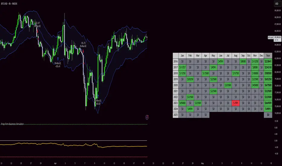
Prop Firm Business SimulatorThe prop firm business simulator is exactly what it sounds like. It's a plug and play tool to test out any tradingview strategy and simulate hypothetical performance on CFD Prop Firms.
Now what is a modern day CFD Prop Firm?
These companies sell simulated trading challenges for a challenge fee. If you complete the challenge you get access to simulated capital and you get a portion of the profits you make on those accounts payed out.
I've included some popular firms in the code as presets so it's easy to simulate them. Take into account that this info will likely be out of date soon as these prices and challenge conditions change.
Also, this tool will never be able to 100% simulate prop firm conditions and all their rules. All I aim to do with this tool is provide estimations.
Now why is this tool helpful?
Most traders on here want to turn their passion into their full-time career, prop firms have lately been the buzz in the trading community and market themselves as a faster way to reach that goal.
While this all sounds great on paper, it is sometimes hard to estimate how much money you will have to burn on challenge fees and set realistic monthly payout expectations for yourself and your trading. This is where this tool comes in.
I've specifically developed this for traders that want to treat prop firms as a business. And as a business you want to know your monthly costs and income depending on the trading strategy and prop firm challenge you are using.
How to use this tool
It's quite simple you remove the top part of the script and replace it with your own strategy. Make sure it's written in same version of pinescript before you do that.
//--$$$$$$$$$$$$$$$$$$$$$$$$$$$$$$$$$$$$$$$$$$$$$$$$--//--------------------------------------------------------------------------------------------------------------------------$$$$$$
//--$$$$$--Strategy-- --$$$$$$--// ******************************************************************************************************************************
//--$$$$$$$$$$$$$$$$$$$$$$$$$$$$$$$$$$$$$$$$$$$$$$$$--//--------------------------------------------------------------------------------------------------------------------------$$$$$$
length = input.int(20, minval=1, group="Keltner Channel Breakout")
mult = input(2.0, "Multiplier", group="Keltner Channel Breakout")
src = input(close, title="Source", group="Keltner Channel Breakout")
exp = input(true, "Use Exponential MA", display = display.data_window, group="Keltner Channel Breakout")
BandsStyle = input.string("Average True Range", options = , title="Bands Style", display = display.data_window, group="Keltner Channel Breakout")
atrlength = input(10, "ATR Length", display = display.data_window, group="Keltner Channel Breakout")
esma(source, length)=>
s = ta.sma(source, length)
e = ta.ema(source, length)
exp ? e : s
ma = esma(src, length)
rangema = BandsStyle == "True Range" ? ta.tr(true) : BandsStyle == "Average True Range" ? ta.atr(atrlength) : ta.rma(high - low, length)
upper = ma + rangema * mult
lower = ma - rangema * mult
//--Graphical Display--// *-*-*-*-*-*-*-*-*-*-*-*-*-*-*-*-*-*-*-*-*-*-*-*-*-*-*-*-*-*-*-*-*-*-*-*-*-*-*-*-*-*-*-*-*-*-*-*-*-*-*-*-*-*-*-*-*-*-*-*-*-*-*-*-*-*-*-*-*-*-*-*-*-$$$$$$
u = plot(upper, color=#2962FF, title="Upper", force_overlay=true)
plot(ma, color=#2962FF, title="Basis", force_overlay=true)
l = plot(lower, color=#2962FF, title="Lower", force_overlay=true)
fill(u, l, color=color.rgb(33, 150, 243, 95), title="Background")
//--Risk Management--// *-*-*-*-*-*-*-*-*-*-*-*-*-*-*-*-*-*-*-*-*-*-*-*-*-*-*-*-*-*-*-*-*-*-*-*-*-*-*-*-*-*-*-*-*-*-*-*-*-*-*-*-*-*-*-*-*-*-*-*-*-*-*-*-*-*-*-*-*-*-*-*-*-*-$$$$$$
riskPerTradePerc = input.float(1, title="Risk per trade (%)", group="Keltner Channel Breakout")
le = high>upper ? false : true
se = lowlower
strategy.entry('PivRevLE', strategy.long, comment = 'PivRevLE', stop = upper, qty=riskToLots)
if se and upper>lower
strategy.entry('PivRevSE', strategy.short, comment = 'PivRevSE', stop = lower, qty=riskToLots)
The tool will then use the strategy equity of your own strategy and use this to simulat prop firms. Since these CFD prop firms work with different phases and payouts the indicator will simulate the gains until target or max drawdown / daily drawdown limit gets reached. If it reaches target it will go to the next phase and keep on doing that until it fails a challenge.
If in one of the phases there is a reward for completing, like a payout, refund, extra it will add this to the gains.
If you fail the challenge by reaching max drawdown or daily drawdown limit it will substract the challenge fee from the gains.
These gains are then visualised in the calendar so you can get an idea of yearly / monthly gains of the backtest. Remember, it is just a backtest so no guarantees of future income.
The bottom pane (non-overlay) is visualising the performance of the backtest during the phases. This way u can check if it is realistic. For instance if it only takes 1 bar on chart to reach target you are probably risking more than the firm wants you to risk. Also, it becomes much less clear if daily drawdown got hit in those high risk strategies, the results will be less accurate.
The daily drawdown limit get's reset every time there is a new dayofweek on chart.
If you set your prop firm preset setting to "'custom" the settings below that are applied as your prop firm settings. Otherwise it will use one of the template by default it's FTMO 100K.
The strategy I'm using as an example in this script is a simple Keltner Channel breakout strategy. I'm using a 0.05% commission per trade as that is what I found most common on crypto exchanges and it's close to the commissions+spread you get on a cfd prop firm. I'm targeting a 1% risk per trade in the backtest to try and stay within prop firm boundaries of max 1% risk per trade.
Lastly, the original yearly and monthly performance table was developed by Quantnomad and I've build ontop of that code. Here's a link to the original publication:
That's everything for now, hope this indicator helps people visualise the potential of prop firms better or to understand that they are not a good fit for their current financial situation.
MACD Aggressive Scalp SimpleComment on the Script
Purpose and Structure:
The script is a scalping strategy based on the MACD indicator combined with EMA (50) as a trend filter.
It uses the MACD histogram's crossover/crossunder of zero to trigger entries and exits, allowing the trader to capitalize on short-term momentum shifts.
The use of strategy.close ensures that positions are closed when specified conditions are met, although adjustments were made to align with Pine Script version 6.
Strengths:
Simplicity and Clarity: The logic is straightforward and focuses on essential scalping principles (momentum-based entries and exits).
Visual Indicators: The plotted MACD line, signal line, and histogram columns provide clear visual feedback for the strategy's operation.
Trend Confirmation: Incorporating the EMA(50) as a trend filter helps avoid trades that go against the prevailing trend, reducing the likelihood of false signals.
Dynamic Exit Conditions: The conditional logic for closing positions based on weakening momentum (via MACD histogram change) is a good way to protect profits or minimize losses.
Potential Improvements:
Parameter Inputs:
Make the MACD (12, 26, 9) and EMA(50) values adjustable by the user through input statements for better customization during backtesting.
Example:
pine
Copy code
macdFast = input(12, title="MACD Fast Length")
macdSlow = input(26, title="MACD Slow Length")
macdSignal = input(9, title="MACD Signal Line Length")
emaLength = input(50, title="EMA Length")
Stop Loss and Take Profit:
The strategy currently lacks explicit stop-loss or take-profit levels, which are critical in a scalping strategy to manage risk and lock in profits.
ATR-based or fixed-percentage exits could be added for better control.
Position Size and Risk Management:
While the script uses 50% of equity per trade, additional options (e.g., fixed position sizes or risk-adjusted sizes) would be beneficial for flexibility.
Avoid Overlapping Signals:
Add logic to prevent overlapping signals (e.g., opening a new position immediately after closing one on the same bar).
Backtesting Optimization:
Consider adding labels or markers (label.new or plotshape) to visualize entry and exit points on the chart for better debugging and analysis.
The inclusion of performance metrics like max drawdown, Sharpe ratio, or profit factor would help assess the strategy's robustness during backtesting.
Compatibility with Live Trading:
The strategy could be further enhanced with alert conditions using alertcondition to notify the trader of buy/sell signals in real-time.

MadTrend [InvestorUnknown]The MadTrend indicator is an experimental tool that combines the Median and Median Absolute Deviation (MAD) to generate signals, much like the popular Supertrend indicator. In addition to identifying Long and Short positions, MadTrend introduces RISK-ON and RISK-OFF states for each trade direction, providing traders with nuanced insights into market conditions.
Core Concepts
Median and Median Absolute Deviation (MAD)
Median: The middle value in a sorted list of numbers, offering a robust measure of central tendency less affected by outliers.
Median Absolute Deviation (MAD): Measures the average distance between each data point and the median, providing a robust estimation of volatility.
Supertrend-like Functionality
MadTrend utilizes the median and MAD in a manner similar to how Supertrend uses averages and volatility measures to determine trend direction and potential reversal points.
RISK-ON and RISK-OFF States
RISK-ON: Indicates favorable conditions for entering or holding a position in the current trend direction.
RISK-OFF: Suggests caution, signaling RISK-ON end and potential trend weakening or reversal.
Calculating MAD
The mad function calculates the median of the absolute deviations from the median, providing a robust measure of volatility.
// Function to calculate the Median Absolute Deviation (MAD)
mad(series float src, simple int length) =>
med = ta.median(src, length) // Calculate median
abs_deviations = math.abs(src - med) // Calculate absolute deviations from median
ta.median(abs_deviations, length) // Return the median of the absolute deviations
MADTrend Function
The MADTrend function calculates the median and MAD-based upper (med_p) and lower (med_m) bands. It determines the trend direction based on price crossing these bands.
MADTrend(series float src, simple int length, simple float mad_mult) =>
// Calculate MAD (volatility measure)
mad_value = mad(close, length)
// Calculate the MAD-based moving average by scaling the price data with MAD
median = ta.median(close, length)
med_p = median + (mad_value * mad_mult)
med_m = median - (mad_value * mad_mult)
var direction = 0
if ta.crossover(src, med_p)
direction := 1
else if ta.crossunder(src, med_m)
direction := -1
Trend Direction and Signals
Long Position (direction = 1): When the price crosses above the upper MAD band (med_p).
Short Position (direction = -1): When the price crosses below the lower MAD band (med_m).
RISK-ON: When the price moves further in the direction of the trend (beyond median +- MAD) after the initial signal.
RISK-OFF: When the price retraces towards the median, signaling potential weakening of the trend.
RISK-ON and RISK-OFF States
RISK-ON LONG: Price moves above the upper band after a Long signal, indicating strengthening bullish momentum.
RISK-OFF LONG: Price falls back below the upper band, suggesting potential weakness in the bullish trend.
RISK-ON SHORT: Price moves below the lower band after a Short signal, indicating strengthening bearish momentum.
RISK-OFF SHORT: Price rises back above the lower band, suggesting potential weakness in the bearish trend.
Picture below show example RISK-ON periods which can be identified by “cloud”
Note: Highlighted areas on the chart indicating RISK-ON and RISK-OFF periods for both Long and Short positions.
Implementation Details
Inputs and Parameters:
Source (input_src): The price data used for calculations (e.g., close, open, high, low).
Median Length (length): The number of periods over which the median and MAD are calculated.
MAD Multiplier (mad_mult): Determines the distance of the upper and lower bands from the median.
Calculations:
Median and MAD are recalculated each period based on the specified length.
Upper (med_p) and Lower (med_m) Bands are computed by adding and subtracting the scaled MAD from the median.
Visual representation of the indicator on a price chart:
Backtesting and Performance Metrics
The MadTrend indicator includes a Backtesting Mode with a performance metrics table to evaluate its effectiveness compared to a simple buy-and-hold strategy.
Equity Calculation:
Calculates the equity curve based on the signals generated by the indicator.
Performance Metrics:
Metrics such as Mean Returns, Standard Deviation, Sharpe Ratio, Sortino Ratio, and Omega Ratio are computed.
The metrics are displayed in a table for both the strategy and the buy-and-hold approach.
Note: Due to the use of labels and plot shapes, automatic chart scaling may not function ideally in Backtest Mode.
Alerts and Notifications
MadTrend provides alert conditions to notify traders of significant events:
Trend Change Alerts
RISK-ON and RISK-OFF Alerts - Provides real-time notifications about the RISK-ON and RISK-OFF states for proactive trade management.
Customization and Calibration
Default Settings: The provided default settings are experimental and not optimized. They serve as a starting point for users.
Parameter Adjustment: Traders are encouraged to calibrate the indicator's parameters (e.g., length, mad_mult) to suit their specific trading style and the characteristics of the asset being analyzed.
Source Input: The indicator allows for different price inputs (open, high, low, close, etc.), offering flexibility in how the median and MAD are calculated.
Important Notes
Market Conditions: The effectiveness of the MadTrend indicator can vary across different market conditions. Regular calibration is recommended.
Backtest Limitations: Backtesting results are historical and do not guarantee future performance.
Risk Management: Always apply sound risk management practices when using any trading indicator.

TrigWave Suite [InvestorUnknown]The TrigWave Suite combines Sine-weighted, Cosine-weighted, and Hyperbolic Tangent moving averages (HTMA) with a Directional Movement System (DMS) and a Relative Strength System (RSS).
Hyperbolic Tangent Moving Average (HTMA)
The HTMA smooths the price by applying a hyperbolic tangent transformation to the difference between the price and a simple moving average. It also adjusts this value by multiplying it by a standard deviation to create a more stable signal.
// Function to calculate Hyperbolic Tangent
tanh(x) =>
e_x = math.exp(x)
e_neg_x = math.exp(-x)
(e_x - e_neg_x) / (e_x + e_neg_x)
// Function to calculate Hyperbolic Tangent Moving Average
htma(src, len, mul) =>
tanh_src = tanh((src - ta.sma(src, len)) * mul) * ta.stdev(src, len) + ta.sma(src, len)
htma = ta.sma(tanh_src, len)
Sine-Weighted Moving Average (SWMA)
The SWMA applies sine-based weights to historical prices. This gives more weight to the central data points, making it responsive yet less prone to noise.
// Function to calculate the Sine-Weighted Moving Average
f_Sine_Weighted_MA(series float src, simple int length) =>
var float sine_weights = array.new_float(0)
array.clear(sine_weights) // Clear the array before recalculating weights
for i = 0 to length - 1
weight = math.sin((math.pi * (i + 1)) / length)
array.push(sine_weights, weight)
// Normalize the weights
sum_weights = array.sum(sine_weights)
for i = 0 to length - 1
norm_weight = array.get(sine_weights, i) / sum_weights
array.set(sine_weights, i, norm_weight)
// Calculate Sine-Weighted Moving Average
swma = 0.0
if bar_index >= length
for i = 0 to length - 1
swma := swma + array.get(sine_weights, i) * src
swma
Cosine-Weighted Moving Average (CWMA)
The CWMA uses cosine-based weights for data points, which produces a more stable trend-following behavior, especially in low-volatility markets.
f_Cosine_Weighted_MA(series float src, simple int length) =>
var float cosine_weights = array.new_float(0)
array.clear(cosine_weights) // Clear the array before recalculating weights
for i = 0 to length - 1
weight = math.cos((math.pi * (i + 1)) / length) + 1 // Shift by adding 1
array.push(cosine_weights, weight)
// Normalize the weights
sum_weights = array.sum(cosine_weights)
for i = 0 to length - 1
norm_weight = array.get(cosine_weights, i) / sum_weights
array.set(cosine_weights, i, norm_weight)
// Calculate Cosine-Weighted Moving Average
cwma = 0.0
if bar_index >= length
for i = 0 to length - 1
cwma := cwma + array.get(cosine_weights, i) * src
cwma
Directional Movement System (DMS)
DMS is used to identify trend direction and strength based on directional movement. It uses ADX to gauge trend strength and combines +DI and -DI for directional bias.
// Function to calculate Directional Movement System
f_DMS(simple int dmi_len, simple int adx_len) =>
up = ta.change(high)
down = -ta.change(low)
plusDM = na(up) ? na : (up > down and up > 0 ? up : 0)
minusDM = na(down) ? na : (down > up and down > 0 ? down : 0)
trur = ta.rma(ta.tr, dmi_len)
plus = fixnan(100 * ta.rma(plusDM, dmi_len) / trur)
minus = fixnan(100 * ta.rma(minusDM, dmi_len) / trur)
sum = plus + minus
adx = 100 * ta.rma(math.abs(plus - minus) / (sum == 0 ? 1 : sum), adx_len)
dms_up = plus > minus and adx > minus
dms_down = plus < minus and adx > plus
dms_neutral = not (dms_up or dms_down)
signal = dms_up ? 1 : dms_down ? -1 : 0
Relative Strength System (RSS)
RSS employs RSI and an adjustable moving average type (SMA, EMA, or HMA) to evaluate whether the market is in a bullish or bearish state.
// Function to calculate Relative Strength System
f_RSS(rsi_src, rsi_len, ma_type, ma_len) =>
rsi = ta.rsi(rsi_src, rsi_len)
ma = switch ma_type
"SMA" => ta.sma(rsi, ma_len)
"EMA" => ta.ema(rsi, ma_len)
"HMA" => ta.hma(rsi, ma_len)
signal = (rsi > ma and rsi > 50) ? 1 : (rsi < ma and rsi < 50) ? -1 : 0
ATR Adjustments
To minimize false signals, the HTMA, SWMA, and CWMA signals are adjusted with an Average True Range (ATR) filter:
// Calculate ATR adjusted components for HTMA, CWMA and SWMA
float atr = ta.atr(atr_len)
float htma_up = htma + (atr * atr_mult)
float htma_dn = htma - (atr * atr_mult)
float swma_up = swma + (atr * atr_mult)
float swma_dn = swma - (atr * atr_mult)
float cwma_up = cwma + (atr * atr_mult)
float cwma_dn = cwma - (atr * atr_mult)
This adjustment allows for better adaptation to varying market volatility, making the signal more reliable.
Signals and Trend Calculation
The indicator generates a Trend Signal by aggregating the output from each component. Each component provides a directional signal that is combined to form a unified trend reading. The trend value is then converted into a long (1), short (-1), or neutral (0) state.
Backtesting Mode and Performance Metrics
The Backtesting Mode includes a performance metrics table that compares the Buy and Hold strategy with the TrigWave Suite strategy. Key statistics like Sharpe Ratio, Sortino Ratio, and Omega Ratio are displayed to help users assess performance. Note that due to labels and plotchar use, automatic scaling may not function ideally in backtest mode.
Alerts and Visualization
Trend Direction Alerts: Set up alerts for long and short signals
Color Bars and Gradient Option: Bars are colored based on the trend direction, with an optional gradient for smoother visual feedback.
Important Notes
Customization: Default settings are experimental and not intended for trading/investing purposes. Users are encouraged to adjust and calibrate the settings to optimize results according to their trading style.
Backtest Results Disclaimer: Please note that backtest results are not indicative of future performance, and no strategy guarantees success.

Z-Score Weighted Trend System I [InvestorUnknown]The Z-Score Weighted Trend System I is an advanced and experimental trading indicator designed to utilize a combination of slow and fast indicators for a comprehensive analysis of market trends. The system is designed to identify stable trends using slower indicators while capturing rapid market shifts through dynamically weighted fast indicators. The core of this indicator is the dynamic weighting mechanism that utilizes the Z-score of price , allowing the system to respond effectively to significant market movements.
Dynamic Z-Score-Based Weighting System
The Z-Score Weighted Trend System I utilizes the Z-score of price to assign weights dynamically to fast indicators. This mechanism is designed to capture rapid market shifts at potential turning points, providing timely entry and exit signals.
Traders can choose from two primary weighting mechanisms:
Threshold-Based Weighting: The fast indicators are given weight only when the absolute Z-score exceeds a user-defined threshold. Below this threshold, fast indicators have no impact on the final signal.
Continuous Weighting: By setting the threshold to zero, fast indicators always contribute to the final signal, regardless of Z-score levels. However, this increases the likelihood of false signals during ranging or low-volatility markets
// Calculate weight for Fast Indicators based on Z-Score (Slow Indicator weight is kept to 1 for simplicity)
f_zscore_weights(series float z, simple float weight_thre) =>
float fast_weight = na
float slow_weight = na
if weight_thre > 0
if math.abs(z) <= weight_thre
fast_weight := 0
slow_weight := 1
else
fast_weight := 0 + math.sqrt(math.abs(z))
slow_weight := 1
else
fast_weight := 0 + math.sqrt(math.abs(z))
slow_weight := 1
Choice of Z-Score Normalization
Traders have the flexibility to select different Z-score processing methods to better suit their trading preferences:
Raw Z-Score or Moving Average: Traders can opt for either the raw Z-score or a moving average of the Z-score to smooth out fluctuations.
Normalized Z-Score (ranging from -1 to 1) or Z-Score Percentile: The normalized Z-score is simply the raw Z-score divided by 3, while the Z-score percentile utilizes a normal distribution for transformation.
f_zscore_perc(series float zscore_src, simple int zscore_len, simple string zscore_a, simple string zscore_b, simple string ma_type, simple int ma_len) =>
z = (zscore_src - ta.sma(zscore_src, zscore_len)) / ta.stdev(zscore_src, zscore_len)
zscore = switch zscore_a
"Z-Score" => z
"Z-Score MA" => ma_type == "EMA" ? (ta.ema(z, ma_len)) : (ta.sma(z, ma_len))
output = switch zscore_b
"Normalized Z-Score" => (zscore / 3) > 1 ? 1 : (zscore / 3) < -1 ? -1 : (zscore / 3)
"Z-Score Percentile" => (f_percentileFromZScore(zscore) - 0.5) * 2
output
Slow and Fast Indicators
The indicator uses a combination of slow and fast indicators:
Slow Indicators (constant weight) for stable trend identification: DMI (Directional Movement Index), CCI (Commodity Channel Index), Aroon
Fast Indicators (dynamic weight) to identify rapid trend shifts: ZLEMA (Zero-Lag Exponential Moving Average), IIRF (Infinite Impulse Response Filter)
Each indicator is calculated using for-loop methods to provide a smoothed and averaged view of price data over varying lengths, ensuring stability for slow indicators and responsiveness for fast indicators.
Signal Calculation
The final trading signal is determined by a weighted combination of both slow and fast indicators. The slow indicators provide a stable view of the trend, while the fast indicators offer agile responses to rapid market movements. The signal calculation takes into account the dynamic weighting of fast indicators based on the Z-score:
// Calculate Signal (as weighted average)
float sig = math.round(((DMI*slow_w) + (CCI*slow_w) + (Aroon*slow_w) + (ZLEMA*fast_w) + (IIRF*fast_w)) / (3*slow_w + 2*fast_w), 2)
Backtest Mode and Performance Metrics
The indicator features a detailed backtesting mode, allowing traders to compare the effectiveness of their selected settings against a traditional Buy & Hold strategy. The backtesting provides:
Equity calculation based on signals generated by the indicator.
Performance metrics comparing Buy & Hold metrics with the system’s signals, including: Mean, positive, and negative return percentages, Standard deviations, Sharpe, Sortino, and Omega Ratios
// Calculate Performance Metrics
f_PerformanceMetrics(series float base, int Lookback, simple float startDate, bool Annualize = true) =>
// Initialize variables for positive and negative returns
pos_sum = 0.0
neg_sum = 0.0
pos_count = 0
neg_count = 0
returns_sum = 0.0
returns_squared_sum = 0.0
pos_returns_squared_sum = 0.0
neg_returns_squared_sum = 0.0
// Loop through the past 'Lookback' bars to calculate sums and counts
if (time >= startDate)
for i = 0 to Lookback - 1
r = (base - base ) / base
returns_sum += r
returns_squared_sum += r * r
if r > 0
pos_sum += r
pos_count += 1
pos_returns_squared_sum += r * r
if r < 0
neg_sum += r
neg_count += 1
neg_returns_squared_sum += r * r
float export_array = array.new_float(12)
// Calculate means
mean_all = math.round((returns_sum / Lookback), 4)
mean_pos = math.round((pos_count != 0 ? pos_sum / pos_count : na), 4)
mean_neg = math.round((neg_count != 0 ? neg_sum / neg_count : na), 4)
// Calculate standard deviations
stddev_all = math.round((math.sqrt((returns_squared_sum - (returns_sum * returns_sum) / Lookback) / Lookback)) * 100, 2)
stddev_pos = math.round((pos_count != 0 ? math.sqrt((pos_returns_squared_sum - (pos_sum * pos_sum) / pos_count) / pos_count) : na) * 100, 2)
stddev_neg = math.round((neg_count != 0 ? math.sqrt((neg_returns_squared_sum - (neg_sum * neg_sum) / neg_count) / neg_count) : na) * 100, 2)
// Calculate probabilities
prob_pos = math.round((pos_count / Lookback) * 100, 2)
prob_neg = math.round((neg_count / Lookback) * 100, 2)
prob_neu = math.round(((Lookback - pos_count - neg_count) / Lookback) * 100, 2)
// Calculate ratios
sharpe_ratio = math.round((mean_all / stddev_all * (Annualize ? math.sqrt(Lookback) : 1))* 100, 2)
sortino_ratio = math.round((mean_all / stddev_neg * (Annualize ? math.sqrt(Lookback) : 1))* 100, 2)
omega_ratio = math.round(pos_sum / math.abs(neg_sum), 2)
// Set values in the array
array.set(export_array, 0, mean_all), array.set(export_array, 1, mean_pos), array.set(export_array, 2, mean_neg),
array.set(export_array, 3, stddev_all), array.set(export_array, 4, stddev_pos), array.set(export_array, 5, stddev_neg),
array.set(export_array, 6, prob_pos), array.set(export_array, 7, prob_neu), array.set(export_array, 8, prob_neg),
array.set(export_array, 9, sharpe_ratio), array.set(export_array, 10, sortino_ratio), array.set(export_array, 11, omega_ratio)
// Export the array
export_array
//}
Calibration Mode
A Calibration Mode is included for traders to focus on individual indicators, helping them fine-tune their settings without the influence of other components. In Calibration Mode, the user can visualize each indicator separately, making it easier to adjust parameters.
Alerts
The indicator includes alerts for long and short signals when the indicator changes direction, allowing traders to set automated notifications for key market events.
// Alert Conditions
alertcondition(long_alert, "LONG (Z-Score Weighted Trend System)", "Z-Score Weighted Trend System flipped ⬆LONG⬆")
alertcondition(short_alert, "SHORT (Z-Score Weighted Trend System)", "Z-Score Weighted Trend System flipped ⬇Short⬇")
Important Note:
The default settings of this indicator are not optimized for any particular market condition. They are generic starting points for experimentation. Traders are encouraged to use the calibration tools and backtesting features to adjust the system to their specific trading needs.
The results generated from the backtest are purely historical and are not indicative of future results. Market conditions can change, and the performance of this system may differ under different circumstances. Traders and investors should exercise caution and conduct their own research before using this indicator for any trading decisions.
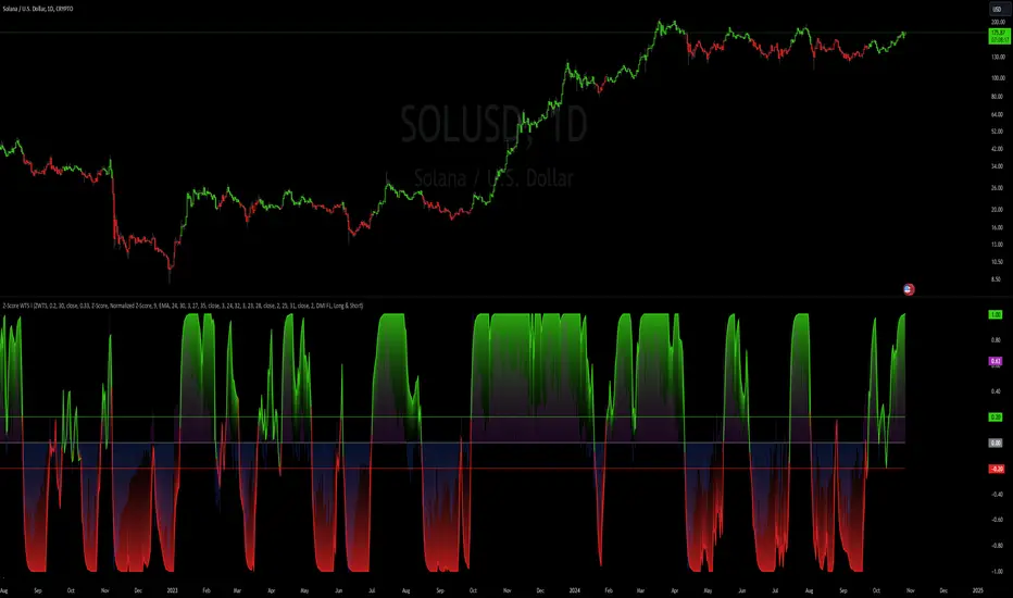
MACD_RSI_trend_followingINFO:
This indicator can be used to build-up a strategy for trading of assets which are currently in trending phase.
My preference is to use it on slowly moving assets like GOLD and on higher timeframes, but practice may show that we find more usefull cases.
This script uses two indicators - MACD and RSI, as the timeframe that those are extracted for is configurable (defaults with the Chart TF, but can be any other selected by the user).
The strategy has the following simple idea - buy if any if the conditions below is true:
The selected TF MACD line crosses above the signal line and the TF RSI is above the user selected trigger value
The selected TF MACD line is above the signal line and the TF RSI crosses above the user selected trigger value
Once we're in position we wait for the selected TF MACD line to cross below the signal line, and then we set a SL at the low of that bar
DETAILS and USAGE:
In the current implementation I find two possible use cases for the indicator:
as a stand-alone indicator on the chart which can also fire alerts that can help to determine if we want to manually enter/exit trades based on them
can be used to connect to the Signal input of the TTS (TempalteTradingStrategy) by jason5480 in order to backtest it, thus effectively turning it into a strategy (instructions below in TTS CONNECTIVITY section)
In the example below we see a position opened at the bar after the buy indicator from the script has been triggered, and then later after the SL indicator from the script has been triggered a SL has been set on the lower wick of the closing candle, and the position eventually got closed once the price hit that level. Note that most of the drawing on the example snapshot below are from the TTS indicator following the buy/sell/SL conditions themseves:
Trading period can be selected from the indicator itself to limit to more interesting periods.
Arrow indications are drawn on the chart to indicate the trading conditions met in the script - green arrow for a buy signal indication and orange for LTF crossunder to indicate setting of SL.
SETTINGS:
Leaving all of the settings as in vanilla use case, as both the MACD and RSI indicator's settings follow the default ones for the stand-alone indicators themselves.
The start-end date is a time filter that can be extermely usefull when backtesting different time periods.
Pesonal preference is using the script on a D/W timeframe, while the indicator is configured to use Monthly chart.
The default value of the RSI filter is left to 50, which can be changed. I.e. if the RSI is above 50 we have a regime filter based on the MACD criteria.
EXTERNAL LIBRARIES:
The script uses a couple of external libraries:
HeWhoMustNotBeNamed/enhanced_ta/14 - collection of TA indicators
jason5480/tts_convention/3 - more details about the Template Trading Strategy below
I would like to highly appreciate and credit the work of both HeWhoMustNotBeNamed and jason5480 for providing them to the community.
TTS SETTINGS (NEEDED IF USED TO BACKTEST WITH TTS):
The TempalteTradingStrategy is a strategy script developed in Pine by jason5480, which I recommend for quick turn-around of testing different ideas on a proven and tested framework
I cannot give enough credit to the developer for the efforts put in building of the infrastructure, so I advice everyone that wants to use it first to get familiar with the concept and by checking
by checking jason5480's profile www.tradingview.com
The TTS itself is extremely functional and have a lot of properties, so its functionality is beyond the scope of the current script -
Again, I strongly recommend to be thoroughly epxlored by everyone that plans on using it.
In the nutshell it is a script that can be feed with buy/sell signals from an external indicator script and based on many configuration options it can determine how to execute the trades.
The TTS has many settings that can be applied, so below I will cover only the ones that differ from the default ones, at least according to my testing - do your own research, you may find something even better :)
The current/latest version that I've been using as of writing and testing this script is TTSv48
Settings which differ from the default ones:
from - False (time filter is from the indicator script itself)
Deal Conditions Mode - External (take enter/exit conditions from an external script)
🔌Signal 🛈➡ - MACD_RSI_trend_following: 🔌Signal to TTSv48 (this is the output from the indicator script, according to the TTS convention)
Sat/Sun - true (for crypto, in order to trade 24/7)
Order Type - STOP (perform stop order)
Distance Method - HHLL (HigherHighLowerLow - in order to set the SL according to the strategy definition from above)
The next are just personal preferenes, you can feel free to experiment according to your trading style
Take Profit Targets - 0 (either 100% in or out, no incremental stepping in or out of positions)
Dist Mul|Len Long/Short- 10 (make sure that we don't close on profitable trades by any reason)
Quantity Method - EQUITY (personal backtesting preference is to consider each backtest as a separate portfolio, so determine the position size by 100% of the allocated equity size)
Equity % - 100 (note above)

Dual_MACD_trendingINFO:
This indicator is useful for trending assets, as my preference is for low-frequency trading, thus using BTCUSD on 1D/1W chart
In the current implementation I find two possible use cases for the indicator:
- as a stand-alone indicator on the chart which can also fire alerts that can help to determine if we want to manually enter/exit trades based on the signals from it (1D/1W is good for non-automated trading)
- can be used to connect to the Signal input of the TTS (TempalteTradingStrategy) by jason5480 in order to backtest it, thus effectively turning it into a strategy (instructions below in TTS CONNECTIVITY section)
Trading period can be selected from the indicator itself to limit to more interesting periods.
Arrow indications are drawn on the chart to indicate the trading conditions met in the script - light green for HTF crossover, dark green for LTF crossover and orange for LTF crossunder.
Note that the indicator performs best in trending assets and markets, and it is advisable to use additional indicators to filter the trading conditions when market/asset is expected to move sideways.
DETAILS:
It uses a couple of MACD indicators - one from the current timeframe and one from a higher timeframe, as the crossover/crossunder cases of the MACD line and the signal line indicate the potential entry/exit points.
The strategy has the following flow:
- If the weekly MACD is positive (MACD line is over the signal line) we have a trading window.
- If we have a trading window, we buy when the daily macd line crosses AND closes above the signal line.
- If we are in a position, we await the daily MACD to cross AND close under the signal line, and only then place a stop loss under the wick of that closing candle.
The user can select both the higher (HTF) and lower (LTF) timeframes. Preferably the lower timeframe should be the one that the Chart is on for better visualization.
If one to decide to use the indicator as a strategy, it implements the following buy and sell criterias, which are feed to the TTS, but can be also manually managed via adding alerts from this indicator.
Since usually the LTF is preceeding the crossover compared to the HTF, then my interpretation of the strategy and flow that it follows is allowing two different ways to enter a trade:
- crossover (and bar close) of the macd over the signal line in the HIGH TIMEFRAME (no need to look at the LOWER TIMEFRMAE)
- crossover (and bar close) of the macd over the signal line in the LOW TIMEFRAME, as in this case we need to check also that the macd line is over the signal line for the HIGH TIMEFRAME as well (like a regime filter)
The exit of the trade is based on the lower timeframe MACD only, as we create a stop loss equal to the lower wick of the bar, once the macd line crosses below the signal line on that timeframe
SETTINGS:
All of the indicator's settings are for the vanilla/general case.
User can set all of the MACD parameters for both the higher and lower (current) timeframes, currently left to default of the MACD stand-alone indicator itself.
The start-end date is a time filter that can be extermely usefull when backtesting different time periods.
TTS SETTINGS (NEEDED IF USED TO BACKTEST WITH TTS)
The TempalteTradingStrategy is a strategy script developed in Pine by jason5480, which I recommend for quick turn-around of testing different ideas on a proven and tested framework
I cannot give enough credit to the developer for the efforts put in building of the infrastructure, so I advice everyone that wants to use it first to get familiar with the concept and by checking
by checking jason5480's profile www.tradingview.com
The TTS itself is extremely functional and have a lot of properties, so its functionality is beyond the scope of the current script -
Again, I strongly recommend to be thoroughly epxlored by everyone that plans on using it.
In the nutshell it is a script that can be feed with buy/sell signals from an external indicator script and based on many configuration options it can determine how to execute the trades.
The TTS has many settings that can be applied, so below I will cover only the ones that differ from the default ones, at least according to my testing - do your own research, you may find something even better :)
The current/latest version that I've been using as of writing and testing this script is TTSv48
Settings which differ from the default ones:
- from - False (time filter is from the indicator script itself)
- Deal Conditions Mode - External (take enter/exit conditions from an external script)
- 🔌Signal 🛈➡ - Dual_MACD: 🔌Signal to TTSv48 (this is the output from the indicator script, according to the TTS convention)
- Sat/Sun - true (for crypto, in order to trade 24/7)
- Order Type - STOP (perform stop order)
- Distance Method - HHLL (HigherHighLowerLow - in order to set the SL according to the strategy definition from above)
The next are just personal preferenes, you can feel free to experiment according to your trading style
- Take Profit Targets - 0 (either 100% in or out, no incremental stepping in or out of positions)
- Dist Mul|Len Long/Short- 10 (make sure that we don't close on profitable trades by any reason)
- Quantity Method - EQUITY (personal backtesting preference is to consider each backtest as a separate portfolio, so determine the position size by 100% of the allocated equity size)
- Equity % - 100 (note above)
EXAMPLES:
If used as a stand-alone indicator, the green arrows on the bottom will represent:
- light green - MACD line crossover signal line in the HTF
- darker green - MACD line crossover signal line in the LTF
- orange - MACD line crossunder signal line in the LTF
I recommend enabling the alerts from the script to cover those cases.
If used as an input to the TTS, we'll get more decorations on the chart from the TTS itself.
In the example below we open a trade on the next day of LTF crossover, then a few days later a crossunder in the LTF occurs, so we set a SL at the low of the wick of this day. Few days later the price doesn't recover and hits that SL, so the position is closed.

Optimized Zhaocaijinbao strategyIntroduction:
The Optimized Zhaocaijinbao strategy is a mid and long-term quantitative trading strategy that combines momentum and trend factors. It generates buy and sell signals by using a combination of exponential moving averages, moving averages, volume and slope indicators. It generates buy signals when the stock is above the 35-day moving average, the trading volume is higher than the 20-day moving average, and the stock is in an upward trend on a weekly timeframe."招财进宝" is a Chinese phrase that can be translated to "Attract Wealth and Bring in Treasure" in English. It is a common expression used to wish for good luck and prosperity in various contexts, such as in business or personal finances.
Highlights:
The strategy has several special optimizations that make it unique.
Firstly, the strategy is optimized for T+1 trading in the Chinese stock market and is only suitable for long positions. The optimizations are also applicable to international stock markets.
Secondly, the trend strategy is optimized to only show indicators on the right side and oscillations. This helps to prevent false signals in choppy markets.
Thirdly, the strategy uses a risk factor for dynamic position sizing to ensure position sizes are adjusted according to the current net asset value and risk preferences. This helps to lower drawdown risks.
The strategy has good resilience even without using stop loss modules in backtesting, making it suitable for trading hourly, 2-hourly, and daily K-line charts (depending on the stock being traded). We recommend experimenting with backtesting using SSE 1-hour or 2-hour or daily Kline charts.
Backtesting outcomes:
The strategy was backtested over the period from October 13th, 2005 to April 14th, 2023, using daily candlestick charts for the commodity code SSE:600763, with a currency of CNY and tick size of 0.01. The strategy used an initial capital of 1,000,000 CNY, with order sizes set to 10% equity and a pyramid of 1 order. The strategy also had a Max Position Size of 0.01 and a Risk Factor of 2.
Here is a summary of the performance of the trading strategy:
Total net profit: 288,577.32 CNY, representing a return of 128.86%
Total number of closed trades: 61
Winning trades: 37, representing a win rate of 60.66%
Profit factor: 2.415
Largest losing trade: 222,021.46 CNY, representing a loss of 14.08%
Average trade: 21,124.22 CNY, representing a return of 3.1%
Average holding period for all trades: 12 days
Conclusion:
In conclusion, the Optimized Zhaocaijinbao strategy is a mid and long-term quantitative trading strategy that combines momentum and trend factors. It is suitable for both Chinese stocks and global stocks. While the Optimized Zhaocaijinbao strategy has performed well in backtesting, it is important to note that past performance is not a guarantee of future results. Traders should conduct their own research and analysis and exercise caution when using any trading strategy.
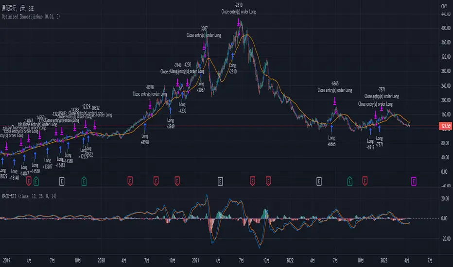
Donchian Trend V1The Donchian Trend strategy is a trend-following approach that uses the Donchian Channels indicator to identify potential entry and exit points in a security. The Donchian Channels are formed by taking the highest high and the lowest low prices over a specified period and plotting them as upper and lower channels around the current price. The width of the channels indicates the level of volatility in the market.
In this strategy, the Donchian Channels are used as a trend filter to determine the direction of the market. When the price is above the upper channel, it suggests an uptrend, and when the price is below the lower channel, it indicates a downtrend. The length of the Donchian Channels is a key parameter in the strategy, as it determines the look-back period for identifying the high and low prices.
Additional Logic: To further refine the entry and exit signals, The script uses two moving averages, a fast one (MA5) and a slow one (MA45), to identify trends and generate trading signals. When the fast moving average crosses above the slow moving average, a buy signal is generated, indicating that the market is trending upwards. Conversely, when the fast moving average crosses below the slow moving average, a sell signal is generated, indicating that the market is trending downwards.
Evaluation: The script was backtested on historical price data for the pair. The backtest results showed that the script was able to generate a net profit of , with a profit factor of and a Sharpe ratio of . The script also includes metrics such as the number of winning and losing trades, the average trade, and the largest winning and losing trades.
The strategy is evaluated based on its net profit, gross profit, gross loss, max run-up, max drawdown, buy & hold return, Sharpe ratio, Sortino ratio, and profit factor. The parameters used in the backtest include a Donchian Channel length of 42, which corresponds to a weekly time with divide of 4h time frame, and a short-term MA of 5 and a long-term MA of 45 for more accurate entry and exit signals.
Disclaimer: This script is for educational and research purposes only and should not be used for trading with real money without further testing and validation. Past performance is not indicative of future results.
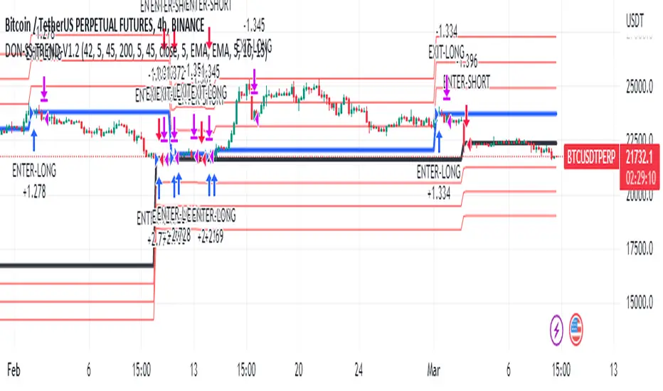
IDAHL | QuantEdgeBIDAHL | QuantEdgeB
🔍 Overview
The IDAHL indicator builds adaptive, volatility-aware threshold bands from two separate ALMA lines—one smoothed from recent highs, the other from recent lows—then uses percentiles of those lines to define a dynamic “high/low” channel. Price crossing above or below that channel triggers clear long/short signals, with on-chart candle coloring, fills, optional labels and even a built-in backtest table.
✨ Key Features
• 📈 Dual ALMA Bands (with DEMA pre-smoothing)
o High ALMA: ALMA applied to DEMA-smoothed highs (high → DEMA(30) → ALMA).
o Low ALMA: ALMA applied to DEMA-smoothed lows (low → DEMA(30) → ALMA).
• 📊 Percentile Thresholds
o Computes a high threshold at the Xth percentile of the High ALMA over a lookback window.
o Computes a low threshold at the Yth percentile of the Low ALMA.
o Shifts each threshold forward by a small period to reduce repainting.
• ⚡ Dynamic Channel Logic
o When price closes above the high percentile line, the “final” threshold flips down to the low percentile line (and vice versa), creating an adaptive channel that only moves when the outer bound is violated.
o Inside the channel, the threshold holds its last value to avoid whipsaw.
• 🎨 Visual & Alerts
o Plots the two percentile lines and fills between them with a color that reflects the current regime (green for long, yellow for neutral, orange for short).
o Colors your candles to match the active signal.
o Optional “Long”/“Short” labels on confirmed flips.
o Alert conditions fire on each long/short crossover.
• 📊 On-Chart Backtest Metrics
o Toggle on a small performance table—complete with win-rate, net P/L, drawdown—from your chosen start date, without any extra code.
⚙️ How It Works
1. Adaptive Smoothing (ALMA)
o Uses ALMA (Arnaud Legoux Moving Average) for smooth, low-lag filtering. In this script, the inputs are additionally pre-smoothed with DEMA(30) to reduce noise before ALMA is applied—improving stability on highs/lows.
2. Percentile Lines
o The High ALMA series feeds a linear-interpolation percentile function to generate the upper bound; the Low ALMA produces the lower bound.
o These lines are offset by a small look-ahead (X bars) to reduce repaint behavior.
3. Channel Logic
o Breakout Flip: When the selected source (default: Close) closes above the upper bound, the active threshold “jumps” to the lower bound—locking in a new channel until price next crosses.
o Breakdown Flip: Conversely, a close below the lower bound flips the threshold to the upper bound.
4. Signal Generation
o Long while the source is above the current “final” threshold.
o Short while below.
o Neutral inside the channel before any flip.
5. Visualization & Alerts
o Dynamic fills between the two percentile lines change hue as the regime flips.
o Candles adopt the regime color.
o Optional pinned “Long”/“Short” labels at flip bars.
o Alerts on every signal crossover of the zero-based regime line.
6. Backtest Table
o From your chosen start date, a mini-table displays cumulative P/L, win rate and drawdown for this strategy—handy for quick in-chart validation.
🎯 Who Should Use It
• Breakout Traders hunting for adaptive channels that auto-recenter on new highs/lows.
• Volatility Traders who want thresholds that expand and contract with market turbulence.
• Trend-Chasers seeking a fresh take on high/low channels with built-in smoothing.
• Systematic Analysts who appreciate on-chart backtesting without leaving TradingView.
⚙️ Default Settings
• ALMA Length: 14
• Percentile Length: 35 bars
• Percentile Lookback Period (offset): 4 bars
• Upper Percentile: 92%
• Lower Percentile: 50%
• Threshold Source: Close
• Visuals: Candle coloring on, labels off by default, “Strategy” palette
• Backtest Table: on by default (toggleable)
• Start Date (Backtest): 09 Oct 2017
📌 Conclusion
IDAHL blends two smooth, low-lag ALMA filters (fed by DEMA-smoothed highs/lows) with percentile-based channel construction for a self-rewiring high/low envelope. It gives you robust breakout/breakdown signals, immediate visual context via colored fills and candles, optional labels, alerts, and even performance stats—everything you need to spot and confirm regime shifts in one compact script.
🔹 Disclaimer : Past performance is not indicative of future results. Always backtest and align settings with your risk tolerance and objectives before live trading.
🔹 Strategic Advice : Always backtest, optimize, and align parameters with your trading objectives and risk tolerance before live trading.

Interest ZonesThis indicator automatically identifies and plots "Interest Zones" around significant pivot highs and lows, representing potential areas of institutional interest, support/resistance, or accumulation/distribution. Zones are dynamically merged when pivots cluster near the same price level and extended for visibility.
How It Works (Technical Methodology)
Pivot Point Detection
The indicator uses Pine Script's ta.pivothigh() and ta.pivotlow() with asymmetric left/right lengths (default left=20, right=13) to detect swing highs and lows. This allows for customizable sensitivity – longer left for stronger confirmation, shorter right for faster detection.
Zone Start Condition (Filtering)
Multiple modes control from which point in history zones begin to be drawn:
"None": All historical pivots (limited by max zones).
"Auto (Start of Day)": Zones only from the beginning of the current trading day (resets daily).
"Manual Date": User-defined fixed date.
"Interactive (Chart)": User-confirmed date via input (useful for backtesting specific periods).
"Last X Bars": Only pivots within the last user-defined number of bars (default 400).
A vertical line marks the start point in date-based modes for visual reference.
Zone Construction
For each valid pivot:
Zone thickness is based on ATR(14) × user-defined multiplier (default 0.3) for dynamic, volatility-adjusted height.
Pivot High zones: Centered below the high (potential supply/resistance).
Pivot Low zones: Centered above the low (potential demand/support).
Zones are drawn as boxes extending to the right, with gray fill and border.
Merge & Overlap Logic
When a new pivot falls inside an existing zone or is very close (within user-defined "Proximity Sensitivity %" of the zone's midpoint, default 1.1%):
The new pivot is merged into the existing zone.
A counter ("x2", "x3", etc.) is displayed on the zone, indicating how many pivots have clustered there.
The zone is strengthened visually (counter text) and extended further right.
This highlights high-interest levels where price repeatedly reversed.
Zone Management
In "None" mode: Only the most recent user-defined max zones are kept (default 5) – oldest deleted automatically.
In other modes: Up to ~490 zones (performance limit), oldest pruned if exceeded.
All zones auto-extend to the right on the last bar for continuous visibility.
Visual Elements
Uniform gray color for all zones (configurable).
Transparent background fill (adjustable).
Counter text in white (configurable) when zones have multiple touches.
Clean, non-directional design – focuses purely on clustered reversal points.
How to Use
Interest Zones highlight price levels where the market has shown repeated respect through multiple swing pivots – often coinciding with institutional order clusters, psychological levels, or hidden support/resistance.
Higher counter values ("x3+", "x5+"): Stronger zones – higher probability of reaction on retest.
Use for:
Potential reversal or bounce areas when price approaches a zone.
Confluence with other tools (order blocks, FVG, volume profile, etc.).
Stop-loss placement beyond zones or take-profit at opposite zones.
Daily reset ("Auto Start of Day"): Ideal for intraday trading – fresh zones each session.
Backtesting: Use "Manual" or "Interactive" date modes to analyze specific historical periods.
"Last X Bars": Good for medium-term swing analysis without full history clutter.
Adjust ATR multiplier for tighter (lower) or wider (higher) zones based on asset volatility. Increase proximity sensitivity for more aggressive merging in ranging markets.
Combine with trend direction, volume, or higher-timeframe structure for best results.
Disclaimer
This indicator is a technical analysis tool and should be used in conjunction with other forms of analysis. Past performance does not guarantee future results. Always use proper risk management.

ORB FX REPLAY - FINAL SAFEHere is the description in English, written to sound professional and meet all the requirements for publishing on TradingView:
Script Description:
Title: ORB Strategy Backtest Pro - Ultra Compatibility
Description: This is an Opening Range Breakout (ORB) strategy specifically designed for professional backtesting. It is optimized to run smoothly on external platforms like FX Replay and TradingView's replay mode.
Key Features:
Custom Session: Automatically calculates the High and Low of a specific time window (default: 10:00 - 10:15 Bucharest/GMT+2).
Impulse Confirmation: Features a "Min Impulse" filter to ensure entries happen on strong momentum, avoiding "fake-outs" near the range boundaries.
Hard Target Management: Designed for "Set & Forget" backtesting. Once a trade is triggered, the script tracks it until it hits either the Stop Loss (SL) or the final Take Profit 3 (TP3).
Visual Projections: Draws clear, real-time lines for Entry, SL, and TP3 on the chart for easy visual tracking.
Automated Statistics: Includes a dynamic label system that tracks Total Trades, Win Count, and Loss Count based on the TP3/SL logic.
Optimized Code: Built using Pine Script v5 with a focus on stability and compatibility, avoiding complex tables that often cause errors on external engines.

Stratégie SMC V18.2 (BTC/EUR FINAL R3 - Tendance)This strategy is an automated implementation of Smart Money Concepts (SMC), designed to operate on the Bitcoin/Euro (BTC/EUR) chart using the 15-minute Timeframe (M15).It focuses on identifying high-probability zones (Order Blocks) after a confirmed Break of Structure (BOS) and a Liquidity Sweep, utilizing an H1/EMA 200 trend filter to only execute trades in the direction of the dominant market flow.Risk management is strict: every trade uses a fixed Risk-to-Reward Ratio (R:R) of 1:3.🧱 Core Logic Components
1. Trend Filter (H1/EMA 200)Objective: To avoid counter-trend entries, which has allowed the success rate to increase to nearly $65\%$ in backtests.Mechanism: A $200$-period EMA is plotted on a higher timeframe (Default: H1/60 minutes).Long (Buy): Entry is only permitted if the current price (M15) is above the trend EMA.Short (Sell): Entry is only permitted if the current price (M15) is below the trend EMA.
2. Order Block (OB) DetectionA potential Order Block is identified on the previous candle if it is
accompanied by an inefficiency (FVG - Fair Value Gap).
3. Advanced SMC ValidationBOS (Break of Structure): A recent BOS must be confirmed by breaking the swing high/low defined by the swing length (Default: 4 M15 candles).Liquidity (Liquidity Sweep): The Order Block zone must have swept recent liquidity (defined by the Liquidity Search Length) within a certain tolerance (Default: $0.1\%$).Point of Interest: The OB must form in a premium zone (for shorts) or a discount zone (for longs) relative to the current swing range (above or below the $50\%$ level of the range).
4. Execution and Risk ManagementEntry: The trade is triggered when the price touches the active Order Block (mitigation).Stop Loss (SL): The SL is fixed at the low of the OB (for longs) or the high of the OB (for shorts).Take Profit (TP): The TP is strictly set at a level corresponding to 3 times the SL distance (R:R 1:3).Lot Sizing: The trade quantity is calculated to risk a fixed amount (Default: 2.00 Euros) per transaction, capped by a Lot Max and Lot Min defined by the user.
Input Parameters (Optimized for BTC/EUR M15)Users can adjust these parameters to modify sensitivity and risk profile. The default values are those optimized for the high-performing backtest (Profit Factor $> 3$).ParameterDescriptionDefault Value (M15)Long. Swing (BOS)Candle length used to define the swing (and thus the BOS).4Long. Recherche Liq.Number of candles to scan to confirm a liquidity sweep.7Tolérance Liq. (%)Price tolerance to validate the liquidity sweep (as a percentage of price).0.1Timeframe TendanceChart timeframe used for the EMA filter (e.g., 60 = H1).60 (H1)Longueur EMA TendancePeriods used for the trend EMA.200Lot Max (Quantité Max BTC)Maximum quantity of BTC the strategy is allowed to trade.0.01Lot Min Réel (Exigence Broker)Minimum quantity required by the broker/exchange.0.00001

Smart Money Concepts [XoRonX]# Smart Money Concepts (SMC) - Advanced Trading Indicator
## 📊 Deskripsi
**Smart Money Concepts ** adalah indicator trading komprehensif yang menggabungkan konsep Smart Money Trading dengan berbagai alat teknikal analisis modern. Indicator ini dirancang untuk membantu trader mengidentifikasi pergerakan institusional (smart money), struktur pasar, zona supply/demand, dan berbagai sinyal trading penting.
Indicator ini mengintegrasikan multiple timeframe analysis, order blocks detection, fair value gaps, fibonacci retracement, volume profile, RSI multi-timeframe, dan moving averages dalam satu platform yang powerful dan mudah digunakan.
---
## 🎯 Fitur Utama
### 1. **Smart Money Structure**
- **Internal Structure** - Struktur pasar jangka pendek untuk entry presisi
- **Swing Structure** - Struktur pasar jangka panjang untuk trend analysis
- **BOS (Break of Structure)** - Konfirmasi kelanjutan trend
- **CHoCH (Change of Character)** - Deteksi potensi reversal
### 2. **Order Blocks**
- **Internal Order Blocks** - Zona demand/supply jangka pendek
- **Swing Order Blocks** - Zona demand/supply jangka panjang
- Filter otomatis berdasarkan volatilitas (ATR/Range)
- Mitigation tracking (High/Low atau Close)
- Customizable display (jumlah order blocks yang ditampilkan)
### 3. **Equal Highs & Equal Lows (EQH/EQL)**
- Deteksi otomatis equal highs/lows
- Indikasi liquidity zones
- Threshold adjustment untuk sensitivitas
- Visual lines dan labels
### 4. **Fair Value Gaps (FVG)**
- Multi-timeframe FVG detection
- Auto threshold filtering
- Bullish & Bearish FVG boxes
- Extension control
- Color customization
### 5. **Premium & Discount Zones**
- Premium Zone (75-100% dari range)
- Equilibrium Zone (47.5-52.5% dari range)
- Discount Zone (0-25% dari range)
- Auto-update berdasarkan swing high/low
### 6. **Fibonacci Retracement**
- **Equilibrium to Discount** - Fib dari EQ ke discount zone
- **Equilibrium to Premium** - Fib dari EQ ke premium zone
- **Discount to Premium** - Fib full range
- Reverse option
- Show/hide lines
- Custom colors
### 7. **Volume Profile (VRVP)**
- Visible Range Volume Profile
- Point of Control (POC)
- Value Area (70% volume)
- Auto-adjust rows
- Placement options (Left/Right)
- Width customization
### 8. **RSI Multi-Timeframe**
- Monitor 3 timeframes sekaligus
- Overbought/Oversold signals
- Visual table display
- Color-coded signals (Red OB, Green OS)
- Customizable position & size
### 9. **Moving Averages**
- 3 Moving Average lines
- Pilihan tipe: EMA, SMA, WMA
- Automatic/Manual period mode
- Individual color & width settings
- Cross alerts (MA vs MA, Price vs MA)
### 10. **Multi-Timeframe Levels**
- Support up to 5 different timeframes
- Previous high/low levels
- Custom line styles
- Color customization
### 11. **Candle Color**
- Color candles berdasarkan trend
- Bullish = Green, Bearish = Red
- Optional toggle
---
## 🛠️ Cara Penggunaan
### **A. Setup Awal**
1. **Tambahkan Indicator ke Chart**
- Buka TradingView
- Klik "Indicators" → "My Scripts" atau paste code
- Pilih "Smart Money Concepts "
2. **Pilih Mode Display**
- **Historical**: Tampilkan semua struktur (untuk backtesting)
- **Present**: Hanya tampilkan struktur terbaru (clean chart)
3. **Pilih Style**
- **Colored**: Warna berbeda untuk bullish/bearish
- **Monochrome**: Tema warna abu-abu
---
### **B. Penggunaan Fitur**
#### **1. Smart Money Structure**
**Internal Structure (Real-time):**
- ✅ Aktifkan "Show Internal Structure"
- Pilih tampilan: All, BOS only, atau CHoCH only
- Gunakan untuk entry timing presisi
- Filter confluence untuk mengurangi noise
**Swing Structure:**
- ✅ Aktifkan "Show Swing Structure"
- Pilih tampilan struktur bullish/bearish
- Adjust "Swings Length" (default: 50)
- Gunakan untuk konfirmasi trend utama
**Tips:**
- BOS = Konfirmasi trend continuation
- CHoCH = Warning untuk possible reversal
- Tunggu price retest ke order block setelah BOS
---
#### **2. Order Blocks**
**Setup:**
- ✅ Aktifkan Internal/Swing Order Blocks
- Set jumlah blocks yang ditampil (1-20)
- Pilih filter: ATR atau Cumulative Mean Range
- Pilih mitigation: Close atau High/Low
**Cara Trading:**
1. Tunggu BOS/CHoCH terbentuk
2. Identifikasi order block terdekat
3. Wait for price pullback ke order block
4. Entry saat price respek order block (rejection)
5. Stop loss di bawah/atas order block
6. Target: swing high/low berikutnya
**Color Code:**
- 🔵 Light Blue = Internal Bullish OB
- 🔴 Light Red = Internal Bearish OB
- 🔵 Dark Blue = Swing Bullish OB
- 🔴 Dark Red = Swing Bearish OB
---
#### **3. Equal Highs/Lows (EQH/EQL)**
**Setup:**
- ✅ Aktifkan "Equal High/Low"
- Set "Bars Confirmation" (default: 3)
- Adjust threshold (0-0.5, default: 0.1)
**Interpretasi:**
- EQH = Liquidity di atas, kemungkinan sweep lalu dump
- EQL = Liquidity di bawah, kemungkinan sweep lalu pump
- Biasanya smart money akan grab liquidity sebelum move besar
**Trading Strategy:**
- Wait for EQH/EQL formation
- Anticipate liquidity grab
- Entry setelah sweep dengan konfirmasi (order block, FVG, CHoCH)
---
#### **4. Fair Value Gaps (FVG)**
**Setup:**
- ✅ Aktifkan "Fair Value Gaps"
- Pilih timeframe (default: chart timeframe)
- Enable/disable auto threshold
- Set extension bars
**Cara Trading:**
1. Bullish FVG = Support zone untuk buy
2. Bearish FVG = Resistance zone untuk sell
3. Price tends to fill FVG (retest)
4. Entry saat price kembali ke FVG
5. Partial fill = valid, full fill = invalidated
**Tips:**
- FVG + Order Block = High probability setup
- Multi-timeframe FVG lebih kuat
- Unfilled FVG = strong momentum
---
#### **5. Premium & Discount Zones**
**Setup:**
- ✅ Aktifkan "Premium/Discount Zones"
- Zones akan auto-update berdasarkan swing high/low
**Interpretasi:**
- 🟢 **Discount Zone** = Area BUY (price murah)
- ⚪ **Equilibrium** = Neutral (50%)
- 🔴 **Premium Zone** = Area SELL (price mahal)
**Trading Strategy:**
- BUY dari discount zone
- SELL dari premium zone
- Avoid trading di equilibrium
- Combine dengan structure confirmation
---
#### **6. Fibonacci Retracement**
**Setup:**
- Pilih Fib yang ingin ditampilkan:
- Equilibrium to Discount
- Equilibrium to Premium
- Discount to Premium
- Toggle show lines
- Enable reverse jika perlu
- Custom colors
**Key Levels:**
- 0.236 = Shallow retracement
- 0.382 = Common retracement
- 0.5 = 50% golden level
- 0.618 = Golden ratio (penting!)
- 0.786 = Deep retracement
**Cara Pakai:**
- 0.618-0.786 = Ideal entry zone dalam trend
- Combine dengan order blocks
- Wait for confirmation candle
---
#### **7. Volume Profile (VRVP)**
**Setup:**
- ✅ Aktifkan "Show Volume Profile"
- Set jumlah rows (10-100)
- Adjust width (5-50%)
- Pilih placement (Left/Right)
- Enable POC dan Value Area
**Interpretasi:**
- **POC (Point of Control)** = Harga dengan volume tertinggi = magnet
- **Value Area** = 70% volume = fair price range
- **Low Volume Nodes** = Weak support/resistance
- **High Volume Nodes** = Strong support/resistance
**Trading:**
- POC acts as support/resistance
- Price tends to return to POC
- Breakout dari Value Area = momentum
---
#### **8. RSI Multi-Timeframe**
**Setup:**
- ✅ Aktifkan "Show RSI Table"
- Set 3 timeframes (default: chart, 5m, 15m)
- Set RSI period (default: 14)
- Set Overbought level (default: 70)
- Set Oversold level (default: 30)
- Pilih posisi & ukuran table
**Interpretasi:**
- 🟢 **OS (Oversold)** = RSI ≤ 30 = Kondisi jenuh jual
- 🔴 **OB (Overbought)** = RSI ≥ 70 = Kondisi jenuh beli
- **-** = Neutral zone
**Trading Strategy:**
1. Multi-timeframe alignment = strong signal
2. OS + Bullish structure = BUY signal
3. OB + Bearish structure = SELL signal
4. Divergence RSI vs Price = reversal warning
**Contoh:**
- TF1: OS, TF2: OS, TF3: OS + Price di discount zone = STRONG BUY
---
#### **9. Moving Averages**
**Setup:**
- Pilih MA Type: EMA, SMA, atau WMA (berlaku untuk ketiga MA)
- Pilih Period Mode: Automatic atau Manual
- Set period untuk MA 1, 2, 3 (default: 20, 50, 100)
- Custom color & width per MA
- ✅ Enable Cross Alerts
**Interpretasi:**
- **Golden Cross** = MA fast cross above MA slow = Bullish
- **Death Cross** = MA fast cross below MA slow = Bearish
- Price above all MAs = Strong uptrend
- Price below all MAs = Strong downtrend
**Trading Strategy:**
1. MA1 (20) = Short-term trend
2. MA2 (50) = Medium-term trend
3. MA3 (100) = Long-term trend
**Entry Signals:**
- Price bounce dari MA dalam trend = continuation
- MA cross dengan konfirmasi structure = entry
- Multiple MA confluence = strong support/resistance
**Alerts Available:**
- MA1 cross MA2/MA3
- MA2 cross MA3
- Price cross any MA
---
#### **10. Multi-Timeframe Levels**
**Setup:**
- Enable HTF Level 1-5
- Set timeframes (contoh: 5m, 1H, 4H, D, W)
- Pilih line style (solid/dashed/dotted)
- Custom colors
**Cara Pakai:**
- Previous high/low dari HTF = strong S/R
- Breakout HTF level = significant move
- Multiple HTF levels confluence = major zone
---
### **C. Trading Setup Combination**
#### **Setup 1: High Probability Buy (Bullish)**
1. ✅ Swing structure: Bullish BOS
2. ✅ Price di Discount Zone
3. ✅ Pullback ke Bullish Order Block
4. ✅ Bullish FVG di bawah
5. ✅ RSI Multi-TF: Oversold
6. ✅ Price bounce dari MA
7. ✅ POC/Value Area support
8. ✅ Fibonacci 0.618-0.786 retracement
**Entry:** Saat price reject dari order block dengan confirmation candle
**Stop Loss:** Below order block
**Target:** Swing high atau premium zone
---
#### **Setup 2: High Probability Sell (Bearish)**
1. ✅ Swing structure: Bearish BOS
2. ✅ Price di Premium Zone
3. ✅ Pullback ke Bearish Order Block
4. ✅ Bearish FVG di atas
5. ✅ RSI Multi-TF: Overbought
6. ✅ Price reject dari MA
7. ✅ POC/Value Area resistance
8. ✅ Fibonacci 0.618-0.786 retracement
**Entry:** Saat price reject dari order block dengan confirmation candle
**Stop Loss:** Above order block
**Target:** Swing low atau discount zone
---
#### **Setup 3: Liquidity Grab (EQH/EQL)**
1. ✅ Identifikasi EQH atau EQL
2. ✅ Wait for liquidity sweep
3. ✅ Konfirmasi dengan CHoCH
4. ✅ Order block terbentuk setelah sweep
5. ✅ Entry saat retest order block
---
### **D. Tips & Best Practices**
**Risk Management:**
- Selalu gunakan stop loss
- Risk 1-2% per trade
- Risk:Reward minimum 1:2
- Jangan over-leverage
**Confluence adalah Kunci:**
- Minimal 3-4 konfirmasi sebelum entry
- Lebih banyak konfirmasi = higher probability
- Quality over quantity
**Timeframe Analysis:**
- HTF (Higher Timeframe) = Trend direction
- LTF (Lower Timeframe) = Entry timing
- Align dengan HTF trend
**Backtesting:**
- Gunakan mode "Historical"
- Test strategy di berbagai market condition
- Record dan analyze hasil
**Market Condition:**
- Trending market = Follow BOS, use order blocks
- Ranging market = Use premium/discount zones, EQH/EQL
- High volatility = Wider stops, wait for clear structure
**Avoid:**
- Trading di equilibrium zone
- Entry tanpa konfirmasi
- Fighting the trend
- Overleveraging
- Emotional trading
---
## 📈 Recommended Settings
### **For Scalping (1m - 5m):**
- Internal Structure: ON
- Swing Structure: OFF
- Order Blocks: Internal only
- RSI Timeframes: 1m, 5m, 15m
- MA Periods: 9, 21, 50
### **For Day Trading (15m - 1H):**
- Internal Structure: ON
- Swing Structure: ON
- Order Blocks: Both
- RSI Timeframes: 15m, 1H, 4H
- MA Periods: 20, 50, 100
### **For Swing Trading (4H - D):**
- Internal Structure: OFF
- Swing Structure: ON
- Order Blocks: Swing only
- RSI Timeframes: 4H, D, W
- MA Periods: 20, 50, 200
---
## ⚠️ Disclaimer
Indicator ini adalah alat bantu analisis teknikal. Tidak ada indicator yang 100% akurat. Selalu:
- Lakukan analisa fundamental
- Gunakan proper risk management
- Praktik di demo account terlebih dahulu
- Trading memiliki resiko, trade at your own risk
---
## 📝 Version Info
**Version:** 5.0
**Platform:** TradingView Pine Script v5
**Author:** XoRonX
**Max Labels:** 500
**Max Lines:** 500
**Max Boxes:** 500
---
## 🔄 Updates & Support
Untuk update, bug reports, atau pertanyaan:
- Check documentation regularly
- Test new features in replay mode
- Backup your settings before updates
---
## 🎓 Learning Resources
**Recommended Study:**
1. Smart Money Concepts (SMC) basics
2. Order blocks theory
3. Liquidity concepts
4. ICT (Inner Circle Trader) concepts
5. Volume profile analysis
6. Multi-timeframe analysis
**Practice:**
- Start with higher timeframes
- Master one concept at a time
- Keep a trading journal
- Review your trades weekly
---
**Happy Trading! 🚀📊**
_Remember: The best indicator is your own analysis and discipline._

Position Size & Drawdown ManagerThis tool is designed to help traders dynamically adjust their position size and drawdown expectations as their trading capital changes over time. It provides a simple and intuitive way to translate backtest results into real-world position sizing decisions.
Purpose and Functionality
The indicator uses your original backtest parameters — including base capital, base drawdown percentage, and base position size — and your current account balance to calculate how your risk profile changes. It presents two main scenarios:
Lock Drawdown %: Keeps your original drawdown percentage fixed and calculates the new position size required.
Lock Position Size: Keeps your position size unchanged and shows how your drawdown percentage will shift.
Why it’s useful
Many traders face the challenge of scaling their strategies as their account grows or shrinks. This tool makes it easy to visualize the relationship between position sizing, capital, and drawdown. It’s particularly valuable for risk management, portfolio rebalancing, and maintaining consistent exposure when transitioning from backtest conditions to live trading.
How it works
The calculations are displayed in a clean, color-coded table that updates dynamically. This allows you to instantly see how capital fluctuations impact your expected drawdown or position size. You can toggle between light and dark themes and highlight important cells for clarity.
Practical use case
Combine this tool with your TradingView strategy results to better interpret your backtests and adjust your real-world trade sizes accordingly. It bridges the gap between simulated performance and actual account management.
Chart example
The chart included focuses only on this indicator, showing the output table and visual layout clearly without additional scripts or overlays.

Match on Selectable Percentage Change + RangeIndicator Overview:
Match on Selectable Percentage Change + Range is a powerful analytical tool designed for traders and analysts who want to identify historical price bars that match a specific percentage variation, and then evaluate how price evolved in the following days. It combines precision filtering with visual tabular feedback, making it ideal for pattern recognition, backtesting, and scenario analysis.
What It Does
This indicator scans historical bars to find instances where the percentage change between two consecutive closes matches a user-defined target (± a customizable tolerance). Once matches are found, it displays:
The date of each match (most recent first)
The actual variation searched
The percentage change after 2, 10, 20, and 30 bars
The min-max range (in %) over those same periods
All results are shown in a dynamic table directly on the chart.
Inputs & Controls
Input Description
Which variation do you want to analyze? (%)
Set the target percentage change to look for (e.g. 2.5%)
% deviation from the variation to be considered (%) Define the tolerance range around the target (e.g. ±0.5%)
Bars to analyze (max 9999) Set how many past bars to scan
Show match table Toggle to enable/disable the entire table
Show percentage variations (2d, 10d, 20d, 30d) Toggle to show/hide post-match percentage changes
Show min-max ranges (2d, 10d, 20d, 30d) Toggle to show/hide post-match high/low ranges
Table Structure
Each row in the table represents a historical match. Columns include:
Date: When the match occurred
Variation in: The actual % change that triggered the match
2d / 10d / 20d / 30d: % change after those days
Min-Max 2d / 10d / 20d / 30d: Range of price movement after those days
Color coding helps quickly identify bullish (green) vs bearish (red) outcomes.
Use Cases
Backtesting: See how similar past moves evolved over time
Scenario modeling: Estimate potential outcomes after a known variation
Pattern recognition: Spot recurring setups or volatility clusters
Risk analysis: Understand post-variation drawdowns and upside potential
Tips for Use
Use tighter deviation (e.g. 0.3%) for precision, or wider (e.g. 1%) for broader pattern capture.
Combine with other indicators to validate setups (e.g. volume, RSI, trend filters).
Toggle off variation or range columns to focus only on the metrics you need.
