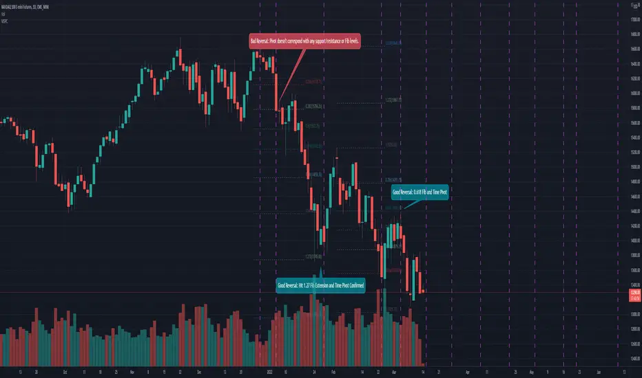
Mean Shift Pivot ClusteringCore Concepts
According to Jeff Greenblatt in his book "Breakthrough Strategies for Predicting Any Market", Fibonacci and Lucas sequences are observed repeated in the bar counts from local pivot highs/lows. They occur from high to high, low to high, high to low, or low to high. Essentially, this phenomenon is observed repeatedly from any pivot points on any time frame. Greenblatt combines this observation with Elliott Waves to predict the price and time reversals. However, I am no Elliottician so it was not easy for me to use this in a practical manner. I decided to only use the bar count projections and ignore the price. I projected a subset of Fibonacci and Lucas sequences along with the Fibonacci ratios from each pivot point. As expected, a projection from each pivot point resulted in a large set of plotted data and looks like a huge gong show of lines. Surprisingly, I did notice clusters and have observed those clusters to be fairly accurate.
Fibonacci Sequence: 1, 2, 3, 5, 8, 13, 21, 34...
Lucas Sequence: 2, 1, 3, 4, 7, 11, 18, 29, 47...
Fibonacci Ratios (converted to whole numbers): 23, 38, 50, 61, 78, 127, 161...
Light Bulb Moment
My eyes may suck at grouping the lines together but what about clustering algorithms? I chose to use a gimped version of Mean Shift because it doesn't require me to know in advance how many lines to expect like K-Means. Mean shift is computationally expensive and with Pinescript's 500ms timeout, I had to make due without the KDE. In other words, I skipped the weighting part but I may try to incorporate it in the future. The code is from Harrison Kinsley . He's a fantastic teacher!
Usage
Search Radius: how far apart should the bars be before they are excluded from the cluster? Try to stick with a figure between 1-5. Too large a figure will give meaningless results.
Pivot Offset: looks left and right X number of bars for a pivot. Same setting as the default TradingView pivot high/low script.
Show Lines Back: show historical predicted lines. (These can change)
Use this script in conjunction with Fibonacci price retracement/extension levels and/or other support/resistance levels. If it's no where near a support/resistance and there's a projected time pivot coming up, it's probably a fake out.
Notes
Re-painting is intended. When a new pivot is found, it will project out the Fib/Lucas sequences so the algorithm will run again with additional information.
The script is for informational and educational purposes only.
Do not use this indicator by itself to trade!
In den Scripts nach "11月1日是什么星座" suchen
Bitcoin Power Law Bands (BTC Power Law) Indicator█ OVERVIEW
The 'Bitcoin Power Law Bands' indicator is a set of three US dollar price trendlines and two price bands for bitcoin , indicating overall long-term trend, support and resistance levels as well as oversold and overbought conditions. The magnitude and growth of the middle (Center) line is determined by double logarithmic (log-log) regression on the entire USD price history of bitcoin . The upper (Resistance) and lower (Support) lines follow the same trajectory but multiplied by respective (fixed) factors. These two lines indicate levels where the price of bitcoin is expected to meet strong long-term resistance or receive strong long-term support. The two bands between the three lines are price levels where bitcoin may be considered overbought or oversold.
All parameters and visuals may be customized by the user as needed.
█ CONCEPTS
Long-term models
Long-term price models have many challenges, the most significant of which is getting the growth curve right overall. No one can predict how a certain market, asset class, or financial instrument will unfold over several decades. In the case of bitcoin , price history is very limited and extremely volatile, and this further complicates the situation. Fortunately for us, a few smart people already had some bright ideas that seem to have stood the test of time.
Power law
The so-called power law is the only long-term bitcoin price model that has a chance of survival for the years ahead. The idea behind the power law is very simple: over time, the rapid (exponential) initial growth cannot possibly be sustained (see The seduction of the exponential curve for a fun take on this). Year-on-year returns, therefore, must decrease over time, which leads us to the concept of diminishing returns and the power law. In this context, the power law translates to linear growth on a chart with both its axes scaled logarithmically. This is called the log-log chart (as opposed to the semilog chart you see above, on which only one of the axes - price - is logarithmic).
Log-log regression
When both price and time are scaled logarithmically, the power law leads to a linear relationship between them. This in turn allows us to apply linear regression techniques, which will find the best-fitting straight line to the data points in question. The result of performing this log-log regression (i.e. linear regression on a log-log scaled dataset) is two parameters: slope (m) and intercept (b). These parameters fully describe the relationship between price and time as follows: log(P) = m * log(T) + b, where P is price and T is time. Price is measured in US dollars , and Time is counted as the number of days elapsed since bitcoin 's genesis block.
DPC model
The final piece of our puzzle is the Dynamic Power Cycle (DPC) price model of bitcoin . DPC is a long-term cyclic model that uses the power law as its foundation, to which a periodic component stemming from the block subsidy halving cycle is applied dynamically. The regression parameters of this model are re-calculated daily to ensure longevity. For the 'Bitcoin Power Law Bands' indicator, the slope and intercept parameters were calculated on publication date (March 6, 2022). The slope of the Resistance Line is the same as that of the Center Line; its intercept was determined by fitting the line onto the Nov 2021 cycle peak. The slope of the Support Line is the same as that of the Center Line; its intercept was determined by fitting the line onto the Dec 2018 trough of the previous cycle. Please see the Limitations section below on the implications of a static model.
█ FEATURES
Inputs
• Parameters
• Center Intercept (b) and Slope (m): These log-log regression parameters control the behavior of the grey line in the middle
• Resistance Intercept (b) and Slope (m): These log-log regression parameters control the behavior of the red line at the top
• Support Intercept (b) and Slope (m): These log-log regression parameters control the behavior of the green line at the bottom
• Controls
• Plot Line Fill: N/A
• Plot Opportunity Label: Controls the display of current price level relative to the Center, Resistance and Support Lines
Style
• Visuals
• Center: Control, color, opacity, thickness, price line control and line style of the Center Line
• Resistance: Control, color, opacity, thickness, price line control and line style of the Resistance Line
• Support: Control, color, opacity, thickness, price line control and line style of the Support Line
• Plots Background: Control, color and opacity of the Upper Band
• Plots Background: Control, color and opacity of the Lower Band
• Labels: N/A
• Output
• Labels on price scale: Controls the display of current Center, Resistance and Support Line values on the price scale
• Values in status line: Controls the display of current Center, Resistance and Support Line values in the indicator's status line
█ HOW TO USE
The indicator includes three price lines:
• The grey Center Line in the middle shows the overall long-term bitcoin USD price trend
• The red Resistance Line at the top is an indication of where the bitcoin USD price is expected to meet strong long-term resistance
• The green Support Line at the bottom is an indication of where the bitcoin USD price is expected to receive strong long-term support
These lines envelope two price bands:
• The red Upper Band between the Center and Resistance Lines is an area where bitcoin is considered overbought (i.e. too expensive)
• The green Lower Band between the Support and Center Lines is an area where bitcoin is considered oversold (i.e. too cheap)
The power law model assumes that the price of bitcoin will fluctuate around the Center Line, by meeting resistance at the Resistance Line and finding support at the Support Line. When the current price is well below the Center Line (i.e. well into the green Lower Band), bitcoin is considered too cheap (oversold). When the current price is well above the Center Line (i.e. well into the red Upper Band), bitcoin is considered too expensive (overbought). This idea alone is not sufficient for profitable trading, but, when combined with other factors, it could guide the user's decision-making process in the right direction.
█ LIMITATIONS
The indicator is based on a static model, and for this reason it will gradually lose its usefulness. The Center Line is the most durable of the three lines since the long-term growth trend of bitcoin seems to deviate little from the power law. However, how far price extends above and below this line will change with every halving cycle (as can be seen for past cycles). Periodic updates will be needed to keep the indicator relevant. The user is invited to adjust the slope and intercept parameters manually between two updates of the indicator.
█ RAMBLINGS
The 'Bitcoin Power Law Bands' indicator is a useful tool for users wishing to place bitcoin in a macro context. As described above, the price level relative to the three lines is a rough indication of whether bitcoin is over- or undervalued. Users wishing to gain more insight into bitcoin price trends may follow the author's periodic updates of the DPC model (contact information below).
█ NOTES
The author regularly posts on Twitter using the @DeFi_initiate handle.
█ THANKS
Many thanks to the following individuals, who - one way or another - made the 'Bitcoin Power Law Bands' indicator possible:
• TradingView user 'capriole_charles', whose open-source 'Bitcoin Power Law Corridor' script was the basis for this indicator
• Harold Christopher Burger, whose Bitcoin’s natural long-term power-law corridor of growth article (2019) was the basis for the 'Bitcoin Power Law Corridor' script
• Bitcoin Forum user "Trololo", who posted the original power law model at Logarithmic (non-linear) regression - Bitcoin estimated value (2014)

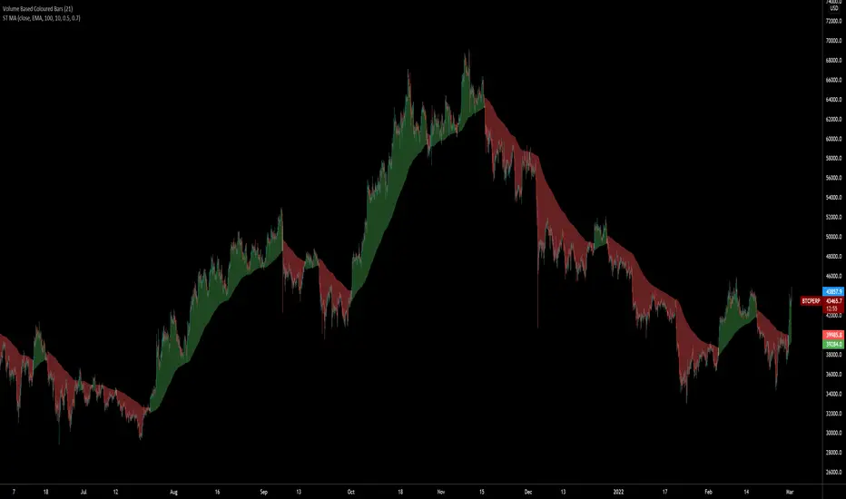
SuperTrended Moving AveragesA different approach to SuperTrend:
adding 100 periods Exponential Moving Average in calculation of SuperTrend and also 0.5 ATR Multiplier to have a clear view of the ongoing trend and also provides significant Supports and Resistances.
Default Moving Average type set as EMA (Exponential Moving Average) but users can choose from 11 different Moving Average types as:
SMA : Simple Moving Average
EMA : Exponential Moving Average
WMA : Weighted Moving Average
DEMA : Double Exponential Moving Average
TMA : Triangular Moving Average
VAR : Variable Index Dynamic Moving Average a.k.a. VIDYA
WWMA : Welles Wilder's Moving Average
ZLEMA : Zero Lag Exponential Moving Average
TSF : True Strength Force
HULL : Hull Moving Average
TILL : Tillson T3 Moving Average
Credits going to @CryptoErge for sharing his development to public.
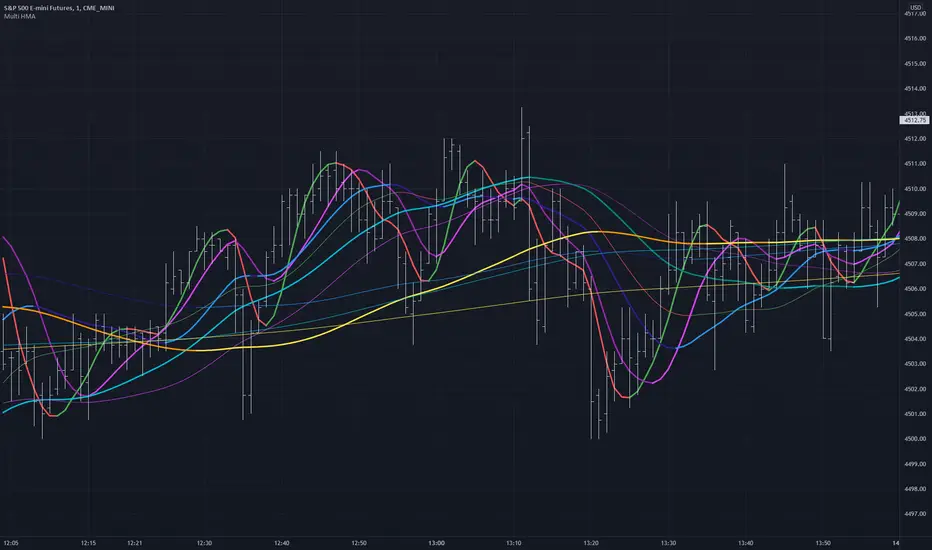
Multiple HMA Original Indicator Script for calculation and color change Hull Ma written and published by huyfibo
I found his version preferable and superior due to the method of mathematics used to get the Hull Ma
I have duplicated huyfibo's calculation for 1 line multiple times, changed variables on each one to create 12 total lines, and customized the color and width of each to help them be identifiable on the 1 minute chart.
This indicator was requested and written for a study to replace multiple SMA's with Hull MAs to compare accuracy as the Hull has much less lag.
As you can see on the above chart, it displays both the 200(1 min) and 1000 ( 5 min) HMA in gold . If user was watching the 1 min chart expecting price to resist at the 200, it would not hold. Although on the 5 min chart it does. This combination gives the user the expectation that price could jump the first line and resist at the second, which it does here.
Combining multiple lines into 1 also to take up much less room at the top of the chart for cleaner visual.
Default values are as such so that the user can have 5 min values displayed on a 1 min chart, as well as the equiv of 200 on the 30 min chart for the 2 and 4 hour.
This is a simply a matter of convenience for the study and can be unchecked to be hidden.
Coded colors and lengths are to visually discern comparable values. Both 1 and 5 min timeframes are the same color, but 1 min timeframe value has larger linewidth
Hull # 10 and 11 are intended for 30 min timeframe and should be unchecked for anything less as their value with be invalid.
All period values, color combinations, and line width can be changed in the the input menu.
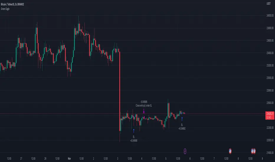
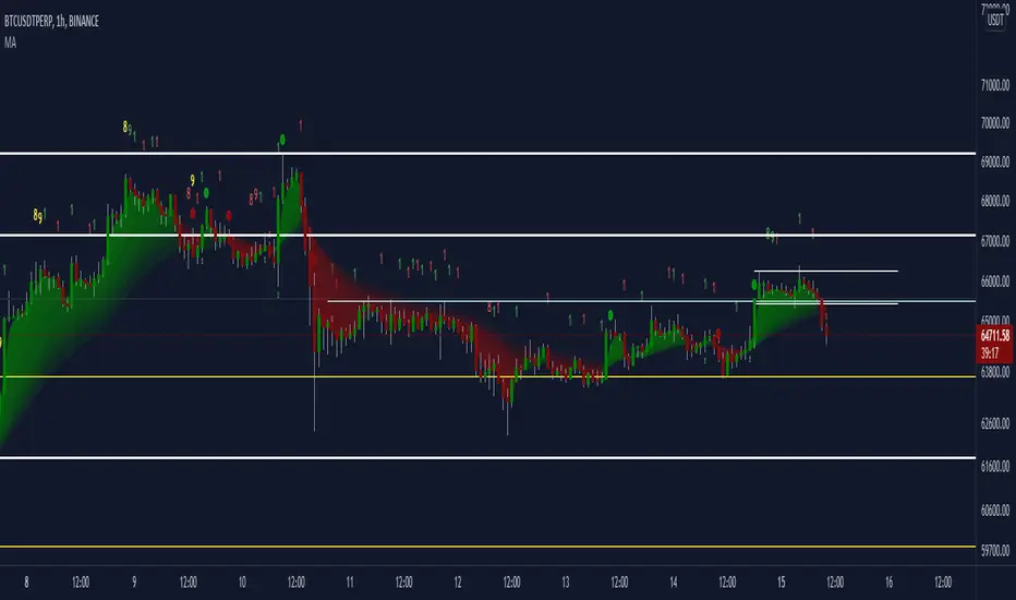
Hourly Bias on BTC in Bullish USA Session “Green Eagle”Name: Hourly Bias on BTC in Bullish USA Session
Category: Hourly Bias
Operating mode: Spot, only long
Trades duration: Intraday, 11 bars
Timeframe: 1H
Suggested usage: When the market is compressed, USA session has a bullish bias.
Entry: enter Long at 15:00 on specific days of the week. There is a volatility filter based on ATR which identifies compression.
Exit: exit at a pre-defined time at 01:00
Usage:
⁃ It can be useful to use alerts or webhooks to automate this strategy.
⁃ This is a core system that can be improved in different ways (e.g. Stop-loss, take-profit, position sizing) or studying more the behaviour in the specific days of the week or short when is red.
Configuration:
- N/A
Backtesting
⁃ Exchange: BINANCE
⁃ Pair: BTCUSDT
⁃ Timeframe: 1H
⁃ Fee 0.075%
⁃ Slippage 2
- Start : 2019-01-06
We decided to release this free BTC strategy.
How you or we can improve? Source code is open so share your ideas!
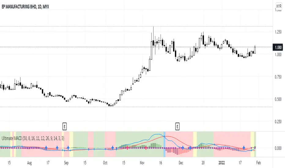
Ultimate MACDThis indicator is an improved version of MACD+RSI (refer to my script list). Basically, this indicator is a combination of several indicators:
1. Fast MACD (preset at 8, 16, 11 - it is my own preference settings and the red and blue line in this indicator are referring to the Fast MACD settings)
2. Slow MACD (preset at 12, 26, 9 - standard settings and the Slow MACD lines are not displayed in this indicator)
3. RSI (preset over value 50)
4. Stochastic (preset overbought at 80, oversold at 20)
How to read:
1. Fast and Slow MACD:
- Two red and blue lines are displaying the Fast MACD lines
- Small blue cross will appear at every crossover of the Fast MACD lines
- Golden Cross 1: Yellow background will appear if only Fast MACD lines are crossing to each other (blue crossover red)
- Golden Cross 2: Green background will appear if both Fast and Slow MACD lines are crossing to each other (blue crossover red but for Slow MACD, I didn't put those lines in this indicator)
- Death Cross 1: Blue background will appear if only Fast MACD lines are crossing to each other (red crossover blue)
- Death Cross 2: Red background will appear if both Fast and Slow MACD lines are crossing to each other (red crossover blue)
2. RSI:
- Purple dots will appear on the center line if RSI value is over 50
3. Stochastic:
- Big Blue cross will appear on the center line if stochastic line are crossing to each other in the oversold area (preset at 20)
- Big Red cross will appear on the center line if stochastic line are crossing to each other in the overbought area (preset at 80)
That's all about this indicator, you can use it based on your own trading style if it suits you. And again I let the script open for anyone to modify it based on your own preferences.
Coppock Curve with Pivot Points and Divergence The Coppock Curve is a long-term price momentum indicator used primarily to recognize major downturns and upturns in a stock market index. It is calculated as a 10-month weighted moving average of the sum of the 14-month rate of change and the 11-month rate of change for the index. It is also known as the "Coppock Guide."
The Coppock formula was introduced in Barron's in 1962 by Edwin Coppock.
The Coppock Curve is a technical indicator that provides long-term buy and sell signals for major stock indexes and related ETFs based on shifts in momentum.
What Does the Coppock Curve Tell You?
The Coppock Curve was originally implemented as a long-term buy and sell indicator for major indices such as the S&P 500 and the Wilshire 5000. Often, it is used with long-term time series such as a candlestick chart, but where each candle contains a month's worth of price information.
The Difference Between the Coppock Curve and Rate of Relative Strength Index (RSI)?
The relative strength index looks at how the current price compares to prior prices, though it is calculated differently than the rate of change (ROC) indicator used in the Coppock Curve calculation. Therefore, these indicators will provide different trade signals and information.
What are those circles?
-These are Divergences. Red for Regular-Bearish. Orange for Hidden-Bearish. Green for Regular-Bullish. Aqua for Hidden-Bullish.
What are those triangles?
- These are Pivots . They show when the VPT oscillator might reverse, this is important to know because many times the price action follows this move.
Please keep in mind that this indicator is a tool and not a strategy, do not blindly trade signals, do your own research first! Use this indicator in conjunction with other indicators to get multiple confirmations.

MEGA_RIBBON_3000🏀 MEGA_RIBBON_3000 is a set of 11 Exponential Moving Averages (EMA), pushing to the limit what's doable with a free member account.

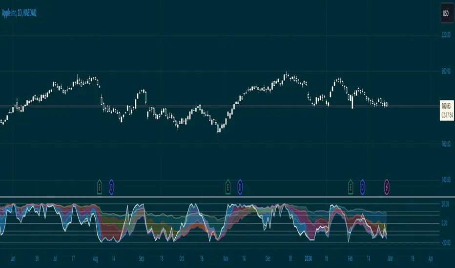
Williams %R & RSI with Multiple PeriodsDESCRIPTION
1. Calculates %R and RSI with multiple period lengths.
1 period length value is defined by User.
8 period length values follow User's selection of classic number sequences, e.g. Fibonacci, Leonardo, Lucas, Narayana, etc.
2. User selects which indicator and periods to display or hide.
DEFAULTS
%R default custom period: 10.
RSI default custom period: 14.
%R & RSI default number sequence periods: Lucas numbers 11, 18, 29, 47, 76, 123, 199, 322.
CALCULATIONS
%R = (period high - most recent period's close price)/(period high - period low)
RSI = 100 - 1 / (100 + RS), where RS = SMMA(up, period) / SMMA(down, period)
PURPOSE
1. Identify price trends.
CREDITS
1. Williams %R technical analysis momentum oscillator by Larry Williams.
2. Wilder's Relative Strength Index technical analysis momentum oscillator by J. Welles Wilder.
3. "Solarized" color scheme by Ethan Schoonover.
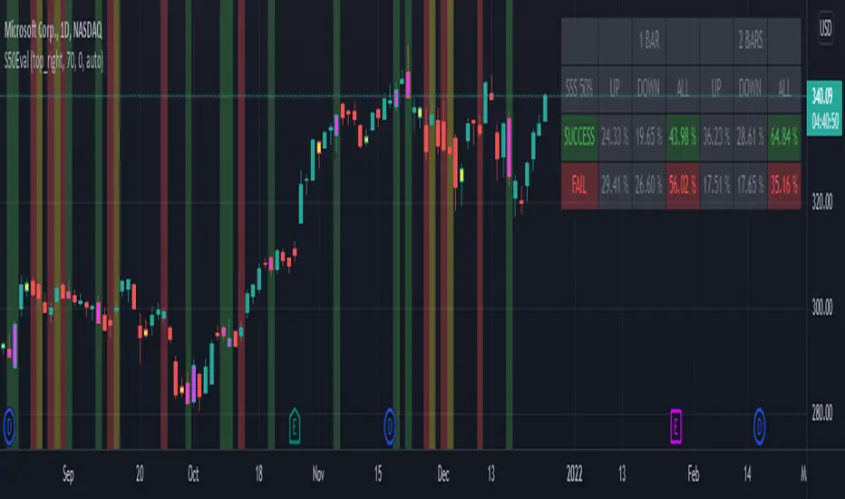
[BM] SSS 50% Rule EvaluatorSara Strat Sniper 50% Rule Evaluator
█ OVERVIEW
This indicator is based on Sara Strat Sniper's - 50% Rule for trading Outside Bars and helps you to evaluate the historical success rate of that rule.
█ FEATURES
Calculation
• You can choose to evaluate only the current bar to see if it forms an outside bar (success) or not (fail), but you can also choose to include the next bar to see if that one forms a compound outside bar.
• You can enable a start and/or end date to limit the calculation period.
Table
• Show or hide the table with the calculation results.
• Show or hide the calculation details (up/down data).
• Position of the table, opacity, cell width and text size can be customized.
Colors
• Table colors can be customized.
• You can choose to show the inside/outside bars in customizable bar colors.
• You can choose to identify successful/failed/recovered outside bars in customizable background colors.
█ LIMITATIONS
• This script uses a special characteristic of the `security()` function allowing the inspection of intrabars — which is not officially supported by TradingView.
• Intrabar inspection only works on some chart timeframes: 5, 10, 15, 30, 45 and 195 minutes, 1, 2, 3, 4, 5, 6, 7 and 8 hours, 1, 2, 3, 4 and 5 days, 1, 2, 3 and 4 weeks, 1, 2, 3, 4, 5, 6, 7, 8, 9, 10, 11 and 12 months. The script’s code can be modified to run on other resolutions.
• There is a limit to how far back intrabar calculations can be performed, and is dependant on both the intrabar resolution and your subscription (which determines the number of available bars).
Swing Trades Validator - The One TraderThis swing trading strategy validator is built on the original strategy taught in my bootcamp for swing traders.
The strategy is simple and follows a trend trading pattern on prices reacting to Exponential Moving Averages over a multiple time-frame analysis.
The details of the strategy are as follows:
- Holding Period : Upto a couple of months
- Time-frames to be analysed : Month - Week - Day
- Trade Execution : Daily Time-frame
Analysis Details:
Step 1 : On the Monthly time-frame, the candle needs to be bullish with the latest close being higher than the opening price of the month.
Step 2 : The price needs to be above the 8ema on the Monthly time-frame.
Step 3 : The 8ema must be above the 20ema on the Monthly time-frame.
The above steps indicate a bullish strength in the instrument on the Monthly time-frame.
Step 4 : On the Weekly time-frame, the candle needs to be bullish with the latest close being higher than the opening price of the week.
Step 5 : The price needs to be above the 8ema on the Weekly time-frame.
Step 6 : The 8ema must be above the 20ema on the Weekly time-frame.
The above steps indicate a bullish strength in the instrument on the Weekly time-frame.
Step 7 : On the Daily time-frame, the candle needs to be bullish with the latest close being higher than the opening price of the day.
Step 8 : The price needs to be above the 8ema on the Daily time-frame.
Step 9 : The 8ema must be above the 20ema on the Daily time-frame.
The above steps indicate a bullish strength in the instrument on the Daily time-frame.
Step 10 : While the 8ema is above the 20ema on the Daily time-frame, the price must be allowed to rise before a pullback is seen towards the moving averages, indicating a bearish move trying to change the trend.
Step 11 : These pullback candles need to form a pattern called the Ring Low with the second pullback candle having a lower high and lower low and the low of the last pullback candle being lesser than or equal to the fat ema on the Daily time-frame.
Step 12 : If the stock is still bullish and the trend is displaying a strength in the underlying bullish direction, then there will be a resumption candle that will have a closing price higher than the previous day's high price.
This trend continuation signal is a confirmation that the instrument will continue in the underlying trend direction and we will be able to enter if this condition is satisfied.
The profit and loss percentages are set at a default 10% as this can be a minimum risk : reward for swing trades on average, but the inputs have been made available to the users in order to adjust the risk : reward to find the most optimum breathing room for each individual stock or instrument. This will give the user a highly custom overview of the strategy on individual instruments based on their volatility and price movements.
The strategy tester will auto back-test this strategy historically and find all the trades that were taken based on this strategy and populate a performance summary.
The most important data in V1.0 of this script are as follows:
1. No. of Trades Taken : We want to see many trades being taken on this strategy in that particular instrument. This shows us a healthy report on the number of winning vs. losing trades.
2. Percentage Profitable : We want to see that this strategy has worked out in the past and is giving us a high probability of return. This in no way an indication that the strategy will definitely work out in the future as well, but gives us an idea of whether or not we should enter this trade.
3. No. of Winning Trades vs. Losing Trades : We would like to see a significantly higher number of winning trades.
4. Avg. # of bars in a trade : This gives us an idea of how long on average we might have to wait to see the results of this strategy either in favor of our reward or against our desired direction. Some trades can be completed in around 15-20 bars on average and some trades have shown to take upto 45 days to reach desired reward. This is in line with our planned holding period, but gives the trader a sense of time and increased level of patience.
The future updates will have more utility of the various elements of the strategy tester and the entire exit strategy will be integrated into the script.
This script is not to be used as a standalone method and must be studied well in order to execute trades. I have not hidden visibility on other time-frames, but since order execution is done on the Daily time-frame, the script must run on the Daily time-frame only.
There are many other factors to be taken into consideration before entering a trade and proper risk management and position sizing rules must be followed.
Our bootcamp participants will use this strategy tester in conjunction with the invite-only Trading Toolkit assigned to them.
The development of this script will be ongoing and all comments and feedback are welcome.

Improved Percent Price Oscillator w/ Colored Candles[C2Trends]The Percent Price Oscillator(PPO) is a momentum oscillator that measures the difference between two moving averages as a percentage of the larger moving average. Similar to the Moving Average Convergence/Divergence(MACD), the PPO is comprised of a signal line, a histogram and a centerline. Signals are generated with signal line crossovers, centerline crossovers, and divergences. Because these signals are no different than those associated with MACD, this indicator can be read exactly as the MACD is read. The main differences between the PPO and MACD are: 1) PPO readings are not subject to the price level of the security. 2) PPO readings for different securities can be compared, even when there are large differences in the price. MACD readings for different securities cannot be compared when there are large differences in price.
PPO Calculations:
Percentage Price Oscillator(PPO): {(12-day EMA - 26-day EMA )/26-day EMA} x 100
Signal Line: 9-day EMA of PPO
PPO Histogram: PPO - Signal Line
iPPO includes everything from standard PPO plus:
1)Plots for PPO/Signal line crosses.
2)Plots for PPO/0 level crosses.
3)PPO/Signal line gap color fill.
4)PPO/0 level gap color fill.
4)Background fill for PPO/Signal line crosses.
5)Background fill for PPO/0 level crosses.
6)Price candles colored based on PPO indicator readings.
7)All plots, lines and fill colors can be turned on/off individually from the 'Input' tab of the iPPO indicator settings menu.
Indicator Notes:
1) When the green PPO line is above the 0 level, intermediate to long-term price momentum can be considered bullish(begins w/yellow cross, green background).
2) When the green PPO line is below the 0 level, intermeidate to long-term price momentum can be considered bearish(begins w/red cross, purple background).
3) Green PPO line above purple Signal line + both lines rising + both lines above 0 level = bullish short-term price momentum(begins w/green dot above 0 level, green highlight).
4) Green PPO line below purple Signal line + both lines falling + both lines above 0 level = loss of short-term bullish price momentum(begins w/purple dot above 0 level, purple highlight).
5) Green PPO line below purple Signal line + both lines falling + both lines below 0 level = bearish short-term price momentum(begins w/purple dot below 0 level, purple highlight).
6) Green PPO line above purple Signal line + both lines rising + both lines below 0 level = loss of short-term bearish price momentum(begins w/green dot below 0 level, green highlight).
7) Price candles are colored lime when the PPO line is above the Signal line and both lines are above the 0 level.
8) Price candles are colored green when the PPO line is below the Signal line and both lines are above the 0 level.
9) Price candles are colored fuschia when the PPO line is below the Signal line and both lines are below the 0 level.
10) Price candles are colored purple when the PPO line is above the Signal line and both lines are below the 0 level.
11) Price candles are colored gray when the green PPO line is within a set % of the 0 level. This value can be set manually in the indicator settings. The default value is 0.25% to ensure
smooth candle color transition between timeframes, charts, sectors and markets. Adjust value up or down if gray candles are absent or too abundant. Gray candles should mostly only appear
during periods of price consolidation(flat/sideways price movement), or just before a significant move up or down in price.

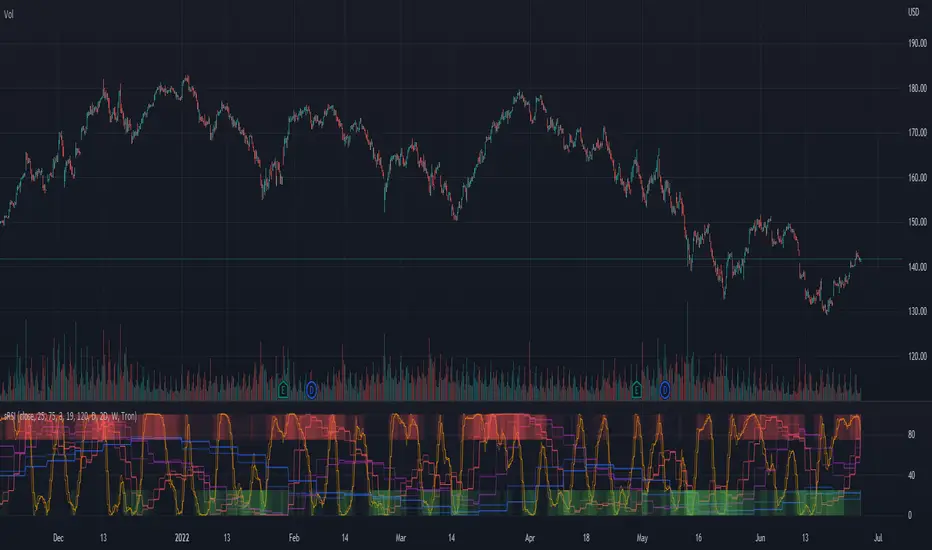
Multi-timeframe Stochastic RSIThe multi-timeframe stochastic RSI utilizes stochastic RSI signals from 11 different time-frames to indicate whether overbought/oversold signals are in agreement or not across time-frames. Ideally traders should enter and exit when conditions are in agreement as indicated by the intensity of the long (green) or short (red) bands at the top and bottom of the indicator. The intensity of the bands indicates how many of the time-frames are currently overbought/oversold.
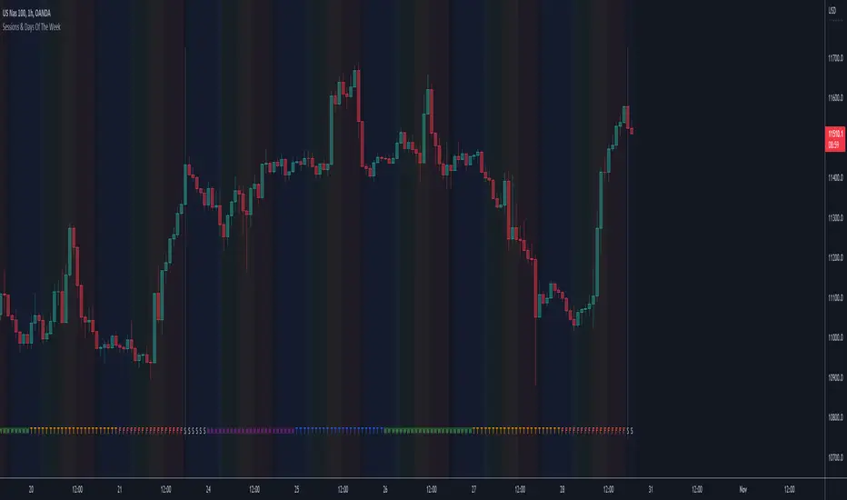
Sessions & Days Of The WeekTraders tend to focus their energy on specific sessions or time periods. This indicator will plot the days of the week, and also highlight the following sessions: Frankfurt (2:00am - 11:00am EST), London (3:00am - 12:00pm EST), New York (8:00am - 5:00pm EST), Sydney (5:00pm - 2:00am EST), Tokyo (7:00pm - 4:00am EST).
It’s important to be aware that Session Open and Close times will vary based on the time of year, as countries shift over to daylight savings time.
S&P Sector CorrelationScript for Macro:
This indicator shows the 9 day average of the correlation of the 11 S&P500 sectors with the security.
Recommend you use the indicator on SPX or SPY, but you can change the values to be compared.
GLHF
- DPT

Moving Average Trend█ OVERVIEW
This is a Moving Average Script that contains both a cloud and a ribbon that has independent MA-type selection.
⬆ green arrow up = up trend flip
⬇ red arrow down = down trend flip
🟢 Green Dot = Potential Long
🔴 Red Dot = Potential Short
█ CONCEPTS
1 — Cloud, like most trading algo, the cloud is made of 8 short term MA , with MA cross and MA cross (longema)
2 — Ribbon, this is by default turned off, the default values , an option in setting to change longema to look for ribbon cross
3 — Sequence, It goes from 1 – 9 at 9 the sequence resets. The sequence changes colour depending on if it’s a down trend(red) or uptrend(green) or an over extended trend (yellow)
Setup definitions
Red sell start = current close < the close 4 candles back
Yellow sell extended = current close < last close and current close < two closes back
Green buy start = current close > the close 4 candles back
Yellow buy extended = current close last close and current close < two closes back
This can help you find when it’s time to get out, or sit out of a choppy trend.
4 - Moving Average types:
sma = Simple Moving Average
ema = Exponential Moving Average
wma = Weighted Moving Average
vwma = Volume Weighted Moving Average
rma = Running Moving Average
alma = Arnaud Legoux Moving Average
hma = Hull Moving Average
jma = Jurik Moving Average
frama-o = frama
frama-m = frama mod
dema = Double Exponential Moving Average
tema = Triple Exponential Moving Average
zlema = Zero lag Exponential Moving Average
smma = Smoothed Moving Average
kma = kaufman Moving Average
tma = triangular Moving Average
gmma = Geometric Mean Moving Average
vida = Variable Index Dynamic Average
cma = Corrective Moving average
rema = Range Exponential Moving average
█ OTHER SECTIONS
• FEATURES: to describe the detailed features of the script, usually arranged in the same order as users will find them in the script's inputs.
• HOW TO USE
• LIMITATIONS: Like with any MA script there is a lag factor associated with is.
• RAMBLINGS: Experiment to your hearts content with all the MA types, I'm impartial to HMA as is
• NOTES: some of the MA's are more taxing, therefore take longer to load, be patience, this is a trimmed down version of an existing invite only script i have
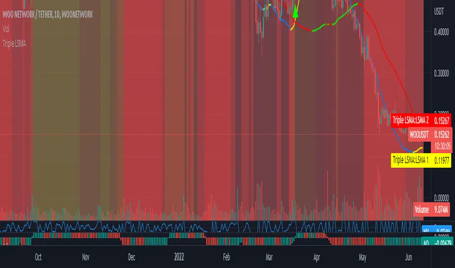
Triple Colored Least Squares Moving Average + Crossover AlertsThis script is forked from the ‘ Double Colored Least Squares Moving Average + Crossover Alerts ‘ from @IronKnightmare.
First release & notes : 2021-11-03.
Overview:
The Least Squares Moving Average is used mainly as a crossover signal to identify bullish or bearish trends. When a shorter duration line cross a longer one a trend can be identified. When multiple lines or the price action cross a longterm trend the confirmation can be further validated. Tradingview contains already some indicators with 1 or two LSMA trendlines that can be configured and toggled.
The original script that I forked had two LSMA lines that could be plotted with other valuable functions, I added a third for further confirmation as some trading systems will use three lines or some combination of those for validation.
Usage:
In inputs
- You will see LSMA 1, LSMA 2 & LSMA 3. The default values are 40, 100 & 400 representing the number of periods plotted by that line : fast, medium and slow changing trendlines will be plotted. The offset value and source are standard for most scripts.
In Style
- You can toggle LSMA 1, 2 or 3 and any combination of those. There are much more possibilities this way.
- For each LSMA, Color 0 & Color 1 are for coloring the slope of the trendline,
- Color 0 for rising slope,
- Color 1 for descending slope.
- The script will automatically color the rise or fall of the trendline accordingly. You can also set one identical color in both slopes for one unique color.
- The ‘ Long Crossover 1 on 2 ’ is a signal for when the LSMA 1 cross over the LSMA 2, usually a shorter periods trendline, more volatile, climbing over the medium term one. A Signal will be traced on the chart at that crossing, you can configure this. The ‘Short Crossover 1 on 2’ is when the LSMA 1 cross under the LSMA 2, a signal will be traced on the chart accordingly.
- The Long Crossover 1 on 3 & Short Crossover 1 on 3 act on the same principle, although the crossing of the fast LSMA on the long / slow LSMA are used. Both can be toggled.
- The ‘ Background Coloring Line 1 : 0-Neutral, 1-Up, 2-Down ’ is an optional background coloring for the LSMA1 line. This can provide additional information at a quick glance, especially if you combine the two other lines backgrounds, the partial transparency will compound.
MAD indicator Enchanced (MADH, inspired by J.Ehlers)This oscillator was inspired by the recent J. Ehler's article (Stocks & Commodities V. 39:11 (24–26): The MAD Indicator, Enhanced by John F. Ehlers). Basically, it shows the difference between two move averages, an "enhancement" made by the author in the last version comes down to replacement SMA to a weighted average that uses Hann windowing. I took the liberty to add colors, ROC line (well, you know, no shorts when ROC's negative and no long's when positive, etc), and optional usage of PVT (price-volume trend) as the source (instead of just price).
Ehlers Error Correcting Exponential Moving Average [CC]The Error Correcting Exponential Moving Average was created by John Ehlers and Ric Way (Stocks & Commodities V. 28:11 (30-35)) and this is an excellent moving average that accurately identifies the trend and sticks with the price during trends or choppy periods pretty well. It looks back to find the best gain setting for each day that returns the smallest difference between the current price and the ema based on the gain setting and uses that day's info in it's total calculations and if there is a zero gain for the day then it is just a classic ema. I have included strong buy and sell signals in addition to normal ones so lighter colors are normal and darker colors are strong. Buy when the line turns green and sell when it turns red.
Let me know if there are any other indicators you would like to see me publish!

TASC 2021.11 MADH Moving Average Difference, Hann█ OVERVIEW
Presented here is code for the "Moving Average Difference, Hann" indicator originally conceived by John Ehlers. The code is also published in the November 2021 issue of Trader's Tips by Technical Analysis of Stocks & Commodities (TASC) magazine.
█ CONCEPTS
By employing a Hann windowed finite impulse response filter (FIR), John Ehlers has enhanced the Moving Average Difference (MAD) to provide an oscillator with exceptional smoothness.
Of notable mention, the wave form of MADH resembles Ehlers' "Reverse EMA" Indicator, formerly revealed in the September 2017 issue of TASC. Many variations of the "Reverse EMA" were published in TradingView's Public Library.
█ FEATURES
Three values in the script's "Settings/Inputs" provide control over the oscillators behavior:
• The price source
• A "Short Length" with a default of 8, to manage the lower band edge of the oscillator
• The "Dominant Cycle", originally set at 27, which appears to be a placeholder for an adaptive control mechanism
Two coloring options are provided for the line's fill:
• "ZeroCross", the default, uses the line's position above/below the zero level. This is the mode used in the top version of MADH on this chart.
• "Momentum" uses the line's up/down state, as shown in the bottom version of the indicator on the chart.
█ NOTES
Calculations
The source price is used in two independent Hann windowed FIR filters having two different periods (lengths) of historical observation for calculation, one being a "Short Length" and the other termed "Dominant Cycle". These are then passed to a "rate of change" calculation and then returned by the reusable function. The secret sauce is that a "windowed Hann FIR filter" is superior tp a generic SMA filter, and that ultimately reveals Ehlers' clever enhancement. We'll have to wait and see what ingenuities Ehlers has next to unleash. Stay tuned...
The `madh()` function code was optimized for computational efficiency in Pine, differing visibly from Ehlers' original formula, but yielding the same results as Ehlers' version.
Background
This indicator has a sibling indicator discussed in the "The MAD Indicator, Enhanced" article by Ehlers. MADH is an evolutionary update from the prior MAD indicator code published in the October 2021 issue of TASC.
Sibling Indicators
• Moving Average Difference (MAD)
• Cycle/Trend Analytics
Related Information
• Cycle/Trend Analytics And The MAD Indicator
• The Reverse EMA Indicator
• Hann Window
• ROC
Join TradingView!

MathSpecialFunctionsTestFunctionsLibrary "MathSpecialFunctionsTestFunctions"
Methods for test functions.
rosenbrock(input_x, input_y) Valley-shaped Rosenbrock function for 2 dimensions: (x,y) -> (1-x)^2 + 100*(y-x^2)^2.
Parameters:
input_x : float, common range within (-5.0, 10.0) or (-2.048, 2.048).
input_y : float, common range within (-5.0, 10.0) or (-2.048, 2.048).
Returns: float
rosenbrock_mdim(samples) Valley-shaped Rosenbrock function for 2 or more dimensions.
Parameters:
samples : float array, common range within (-5.0, 10.0) or (-2.048, 2.048).
Returns: float
himmelblau(input_x, input_y) Himmelblau, a multi-modal function: (x,y) -> (x^2+y-11)^2 + (x+y^2-7)^2
Parameters:
input_x : float, common range within (-6.0, 6.0 ).
input_y : float, common range within (-6.0, 6.0 ).
Returns: float
rastrigin(samples) Rastrigin, a highly multi-modal function with many local minima.
Parameters:
samples : float array, common range within (-5.12, 5.12 ).
Returns: float
drop_wave(input_x, input_y) Drop-Wave, a multi-modal and highly complex function with many local minima.
Parameters:
input_x : float, common range within (-5.12, 5.12 ).
input_y : float, common range within (-5.12, 5.12 ).
Returns: float
ackley(input_x) Ackley, a function with many local minima. It is nearly flat in outer regions but has a large hole at the center.
Parameters:
input_x : float array, common range within (-32.768, 32.768 ).
Returns: float
bohachevsky1(input_x, input_y) Bowl-shaped first Bohachevsky function.
Parameters:
input_x : float, common range within (-100.0, 100.0 ).
input_y : float, common range within (-100.0, 100.0 ).
Returns: float
matyas(input_x, input_y) Plate-shaped Matyas function.
Parameters:
input_x : float, common range within (-10.0, 10.0 ).
input_y : float, common range within (-10.0, 10.0 ).
Returns: float
six_hump_camel(input_x, input_y) Valley-shaped six-hump camel back function.
Parameters:
input_x : float, common range within (-3.0, 3.0 ).
input_y : float, common range within (-2.0, 2.0 ).
Returns: float

MathConstantsUniversalLibrary "MathConstantsUniversal"
Mathematical Constants
SpeedOfLight() Speed of Light in Vacuum: c_0 = 2.99792458e8 (defined, exact; 2007 CODATA)
MagneticPermeability() Magnetic Permeability in Vacuum: mu_0 = 4*Pi * 10^-7 (defined, exact; 2007 CODATA)
ElectricPermittivity() Electric Permittivity in Vacuum: epsilon_0 = 1/(mu_0*c_0^2) (defined, exact; 2007 CODATA)
CharacteristicImpedanceVacuum() Characteristic Impedance of Vacuum: Z_0 = mu_0*c_0 (defined, exact; 2007 CODATA)
GravitationalConstant() Newtonian Constant of Gravitation: G = 6.67429e-11 (2007 CODATA)
PlancksConstant() Planck's constant: h = 6.62606896e-34 (2007 CODATA)
DiracsConstant() Reduced Planck's constant: h_bar = h / (2*Pi) (2007 CODATA)
PlancksMass() Planck mass: m_p = (h_bar*c_0/G)^(1/2) (2007 CODATA)
PlancksTemperature() Planck temperature: T_p = (h_bar*c_0^5/G)^(1/2)/k (2007 CODATA)
PlancksLength() Planck length: l_p = h_bar/(m_p*c_0) (2007 CODATA)
PlancksTime() Planck time: t_p = l_p/c_0 (2007 CODATA)

Vector2OperationsLibrary "Vector2Operations"
functions to handle vector2 operations.
math_fractional(_value) computes the fractional part of the argument value.
Parameters:
_value : float, value to compute.
Returns: float, fractional part.
atan2(_a) Approximation to atan2 calculation, arc tangent of y/ x in the range radians.
Parameters:
_a : vector2 in the form of a array .
Returns: float, value with angle in radians. (negative if quadrante 3 or 4)
set_x(_a, _value) Set the x value of vector _a.
Parameters:
_a : vector2 in the form of a array .
_value : value to replace x value of _a.
Returns: void Modifies vector _a.
set_y(_a, _value) Set the y value of vector _a.
Parameters:
_a : vector in the form of a array .
_value : value to replace y value of _a.
Returns: void Modifies vector _a.
get_x(_a) Get the x value of vector _a.
Parameters:
_a : vector in the form of a array .
Returns: float, x value of the vector _a.
get_y(_a) Get the y value of vector _a.
Parameters:
_a : vector in the form of a array .
Returns: float, y value of the vector _a.
get_xy(_a) Return the tuple of vector _a in the form
Parameters:
_a : vector2 in the form of a array .
Returns:
length_squared(_a) Length of vector _a in the form. , for comparing vectors this is computationaly lighter.
Parameters:
_a : vector in the form of a array .
Returns: float, squared length of vector.
length(_a) Magnitude of vector _a in the form.
Parameters:
_a : vector in the form of a array .
Returns: float, Squared length of vector.
vmin(_a) Lowest element of vector.
Parameters:
_a : vector in the form of a array .
Returns: float
vmax(_a) Highest element of vector.
Parameters:
_a : vector in the form of a array .
Returns: float
from(_value) Assigns value to a new vector x,y elements.
Parameters:
_value : x and y value of the vector. optional.
Returns: float vector.
new(_x, _y) Creates a prototype array to handle vectors.
Parameters:
_x : float, x value of the vector. optional.
_y : float, y number of the vector. optional.
Returns: float vector.
down() Vector in the form . Returns: float vector.
left() Vector in the form . Returns: float vector.
one() Vector in the form . Returns: float vector.
right() Vector in the form . Returns: float vector
up() Vector in the form . Returns: float vector
zero() Vector in the form . Returns: float vector
add(_a, _b) Adds vector _b to _a, in the form
.
Parameters:
_a : vector in the form of a array .
_b : vector in the form of a array .
Returns:
subtract(_a, _b) Subtract vector _b from _a, in the form
.
Parameters:
_a : vector in the form of a array .
_b : vector in the form of a array .
Returns:
multiply(_a, _b) Multiply vector _a with _b, in the form
Parameters:
_a : vector in the form of a array .
_b : vector in the form of a array .
Returns:
divide(_a, _b) Divide vector _a with _b, in the form
Parameters:
_a : vector in the form of a array .
_b : vector in the form of a array .
Returns:
negate(_a) Negative of vector _a, in the form
Parameters:
_a : vector in the form of a array .
Returns:
perp(_a) Perpendicular Vector of _a.
Parameters:
_a : vector in the form of a array .
Returns:
vfloor(_a) Compute the floor of argument vector _a.
Parameters:
_a : vector in the form of a array .
Returns:
fractional(_a) Compute the fractional part of the elements from vector _a.
Parameters:
_a : vector in the form of a array .
Returns:
vsin(_a) Compute the sine of argument vector _a.
Parameters:
_a : vector in the form of a array .
Returns:
equals(_a, _b) Compares two vectors
Parameters:
_a : vector in the form of a array .
_b : vector in the form of a array .
Returns: boolean value representing the equality.
dot(_a, _b) Dot product of 2 vectors, in the form
Parameters:
_a : vector in the form of a array .
_b : vector in the form of a array .
Returns: float
cross_product(_a, _b) cross product of 2 vectors, in the form
Parameters:
_a : vector in the form of a array .
_b : vector in the form of a array .
Returns: float
scale(_a, _scalar) Multiply a vector by a scalar.
Parameters:
_a : vector in the form of a array .
_scalar : value to multiply vector elements by.
Returns: float vector
normalize(_a) Vector _a normalized with a magnitude of 1, in the form.
Parameters:
_a : vector in the form of a array .
Returns: float vector
rescale(_a) Rescale a vector to a new Magnitude.
Parameters:
_a : vector in the form of a array .
Returns:
rotate(_a, _radians) Rotates vector _a by angle value
Parameters:
_a : vector in the form of a array .
_radians : Angle value.
Returns:
rotate_degree(_a, _degree) Rotates vector _a by angle value
Parameters:
_a : vector in the form of a array .
_degree : Angle value.
Returns:
rotate_around(_center, _target, _degree) Rotates vector _target around _origin by angle value
Parameters:
_center : vector in the form of a array .
_target : vector in the form of a array .
_degree : Angle value.
Returns:
vceil(_a, _digits) Ceils vector _a
Parameters:
_a : vector in the form of a array .
_digits : digits to use as ceiling.
Returns:
vpow(_a) Raise both vector elements by a exponent.
Parameters:
_a : vector in the form of a array .
Returns:
distance(_a, _b) vector distance between 2 vectors.
Parameters:
_a : vector in the form of a array .
_b : vector in the form of a array .
Returns: float, distance.
project(_a, _axis) Project a vector onto another.
Parameters:
_a : vector in the form of a array .
_axis : float vector2
Returns: float vector
projectN(_a, _axis) Project a vector onto a vector of unit length.
Parameters:
_a : vector in the form of a array .
_axis : vector in the form of a array .
Returns: float vector
reflect(_a, _b) Reflect a vector on another.
Parameters:
_a : vector in the form of a array .
_b : vector in the form of a array .
Returns: float vector
reflectN(_a, _b) Reflect a vector to a arbitrary axis.
Parameters:
_a : vector in the form of a array .
_b : vector in the form of a array .
Returns: float vector
angle(_a) Angle in radians of a vector.
Parameters:
_a : vector in the form of a array .
Returns: float
angle_unsigned(_a, _b) unsigned degree angle between 0 and +180 by given two vectors.
Parameters:
_a : vector in the form of a array .
_b : vector in the form of a array .
Returns: float
angle_signed(_a, _b) Signed degree angle between -180 and +180 by given two vectors.
Parameters:
_a : vector in the form of a array .
_b : vector in the form of a array .
Returns: float
angle_360(_a, _b) Degree angle between 0 and 360 by given two vectors
Parameters:
_a : vector in the form of a array .
_b : vector in the form of a array .
Returns: float
clamp(_a, _vmin, _vmax) Restricts a vector between a min and max value.
Parameters:
_a : vector in the form of a array .
_vmin : vector in the form of a array .
_vmax : vector in the form of a array .
Returns: float vector
lerp(_a, _b, _rate_of_move) Linearly interpolates between vectors a and b by _rate_of_move.
Parameters:
_a : vector in the form of a array .
_b : vector in the form of a array .
_rate_of_move : float value between (a:-infinity -> b:1.0), negative values will move away from b.
Returns: vector in the form of a array
herp(_a, _b, _rate_of_move) Hermite curve interpolation between vectors a and b by _rate_of_move.
Parameters:
_a : vector in the form of a array .
_b : vector in the form of a array .
_rate_of_move : float value between (a-infinity -> b1.0), negative values will move away from b.
Returns: vector in the form of a array
area_triangle(_a, _b, _c) Find the area in a triangle of vectors.
Parameters:
_a : vector in the form of a array .
_b : vector in the form of a array .
_c : vector in the form of a array .
Returns: float
to_string(_a) Converts vector _a to a string format, in the form "(x, y)"
Parameters:
_a : vector in the form of a array .
Returns: string in "(x, y)" format
vrandom(_max) 2D random value
Parameters:
_max : float vector, vector upper bound
Returns: vector in the form of a array
noise(_a) 2D Noise based on Morgan McGuire @morgan3d
thebookofshaders.com
www.shadertoy.com
Parameters:
_a : vector in the form of a array .
Returns: vector in the form of a array
array_new(_size, _initial_vector) Prototype to initialize a array of vectors.
Parameters:
_size : size of the array.
_initial_vector : vector to be used as default value, in the form of array .
Returns: _vector_array complex Array in the form of a array
array_size(_id) number of vector elements in array.
Parameters:
_id : ID of the array.
Returns: int
array_get(_id, _index) Get the vector in a array, in the form of a array
Parameters:
_id : ID of the array.
_index : Index of the vector.
Returns: vector in the form of a array
array_set(_id, _index, _a) Sets the values vector in a array.
Parameters:
_id : ID of the array.
_index : Index of the vector.
_a : vector, in the form .
Returns: Void, updates array _id.
array_push(_id, _a) inserts the vector at the end of array.
Parameters:
_id : ID of the array.
_a : vector, in the form .
Returns: Void, updates array _id.
array_unshift(_id, _a) inserts the vector at the begining of array.
Parameters:
_id : ID of the array.
_a : vector, in the form .
Returns: Void, updates array _id.
array_pop(_id, _a) removes the last vector of array and returns it.
Parameters:
_id : ID of the array.
_a : vector, in the form .
Returns: vector2, updates array _id.
array_shift(_id, _a) removes the first vector of array and returns it.
Parameters:
_id : ID of the array.
_a : vector, in the form .
Returns: vector2, updates array _id.
array_sum(_id) Total sum of all vectors.
Parameters:
_id : ID of the array.
Returns: vector in the form of a array
array_center(_id) Finds the vector center of the array.
Parameters:
_id : ID of the array.
Returns: vector in the form of a array
array_rotate_points(_id) Rotate Array vectors around origin vector by a angle.
Parameters:
_id : ID of the array.
Returns: rotated points array.
array_scale_points(_id) Scale Array vectors based on a origin vector perspective.
Parameters:
_id : ID of the array.
Returns: rotated points array.
array_tostring(_id, _separator) Reads a array of vectors into a string, of the form " ""
Parameters:
_id : ID of the array.
_separator : string separator for cell splitting.
Returns: string Translated complex array into string.
line_new(_a, _b) 2 vector line in the form.
Parameters:
_a : vector, in the form .
_b : vector, in the form .
Returns:
line_get_a(_line) Start vector of a line.
Parameters:
_line : vector4, in the form .
Returns: float vector2
line_get_b(_line) End vector of a line.
Parameters:
_line : vector4, in the form .
Returns: float vector2
line_intersect(_line1, _line2) Find the intersection vector of 2 lines.
Parameters:
_line1 : line of 2 vectors in the form of a array .
_line2 : line of 2 vectors in the form of a array .
Returns: vector in the form of a array .
draw_line(_line, _xloc, _extend, _color, _style, _width) Draws a line using line prototype.
Parameters:
_line : vector4, in the form .
_xloc : string
_extend : string
_color : color
_style : string
_width : int
Returns: draw line object
draw_triangle(_v1, _v2, _v3, _xloc, _color, _style, _width) Draws a triangle using line prototype.
Parameters:
_v1 : vector4, in the form .
_v2 : vector4, in the form .
_v3 : vector4, in the form .
_xloc : string
_color : color
_style : string
_width : int
Returns: tuple with 3 line objects.
draw_rect(_v1, _size, _angle, _xloc, _color, _style, _width) Draws a square using vector2 line prototype.
Parameters:
_v1 : vector4, in the form .
_size : float
_angle : float
_xloc : string
_color : color
_style : string
_width : int
Returns: tuple with 3 line objects.
