Vega Convexity Engine [PRO]ENGINEERED ASYMMETRY.
This is the flagship Stage 2 Specialist Model of the Vega Crypto Strategies ecosystem.
While the free "Regime Filter" tells you when to trade (filtering out chop), the Convexity Engine tells you how to trade. It activates only when the Regime Filter confirms an Impulse, classifying the specific vector of the market move to maximize risk-adjusted returns.
PRO FEATURES
This script visualizes the output of our Hierarchical Machine Learning Engine:
🚀 Directional Classification:
It does not just say "Buy." It classifies volatility into 4 distinct probability classes:
- EXPLOSION: High-confidence, high-velocity upside (Fat-Tail).
- RALLY: Standard trend continuation.
- PULLBACK: Short-term correction opportunity.
- CRASH: High-confidence downside (Long Squeeze Detection).
🛡️ Dynamic Risk Engine (Intraday Stops):
The "+" markers on your chart represent the Vega Institutional Stop Loss . These levels dynamically adjust based on Average True Range (ATR) and Volatility Z-Scores.
Strategy: If price breaches the "+" marker, the hypothesis is invalidated. Exit immediately.
📊 Institutional HUD:
A professional heads-up display showing the current Regime, Vector, and Risk Deployment status in real-time.
THE PHILOSOPHY
"Convexity" means limited downside with unlimited upside. By combining the Regime Filter (sitting in cash during noise) with Dynamic Stops (cutting losers fast), this engine is designed to capture the "fat tails" of the crypto market distribution.
🔒 HOW TO GET ACCESS
This is an Invite-Only script. It is strictly for members of Vega Crypto Strategies .
To unlock access, please visit the link in the Author Profile below or check our signature. Once subscribed via Whop, your TradingView username will be automatically authorized instantly.
Disclaimer: This tool is for educational purposes only. Past performance is not indicative of future results. Trading cryptocurrencies involves significant risk.
Machinelearning

JINN: A Multi-Paradigm Quantitative Trading and Execution EngineI. Core Philosophy: A Substitute for Static Analysis
JINN (Joint Investment Neural and Network) represents a paradigm shift from static indicators to a living, adaptive analytical ecosystem. Traditional tools provide a fixed snapshot of the market. JINN operates on a fundamentally different premise: it treats the market as a dynamic, regime-driven system. It processes market data through a hierarchical suite of advanced, interacting models, arbitrates their outputs through a rules-based engine, and adapts its own logic in real-time.
It is designed as a complete framework for traders who think in terms of statistical edge, market regimes, probabilistic outcomes, and adaptive risk management.
II. The JINN Branded Architecture: Your Command and Control Centre
JINN’s power emerges from the synergy of its proprietary, branded architectural components. You do not simply "use" JINN; you command its engines.
1. JINN Signal Arbitration (JSA) Engine
The heart of JINN. The JSA is your configurable arbitration desk for weighing evidence from all internal models. As the Head Strategist, you define the entire arbitration philosophy:
• Priority and Weighting : Define a "chain of command". Specify which model's opinion must be considered first and assign custom weights to their outputs, directly controlling the hierarchy of your analytical flow.
• Arbitration Modes :
First Wins: For high-conviction, rapid signal deployment based on your most trusted leading model.
Highest Score: A "best evidence" approach that runs a full analysis and selects the signal with the highest weighted probabilistic backing.
Consensus: An ultra-conservative, "all-clear" mode that requires a unanimous pass from all active models, ensuring maximum confluence.
2. JINN Threshold Fusion (JTF) Engine
Static entry thresholds can be limiting in a dynamic market. The JTF engine replaces them with a robust, adaptive "breathing" channel.
• Kalman Filter Core : A noise-reducing, parametric filter that provides a smooth, responsive centre for the entry bands.
• Exponentially Weighted Quantile (EWQ) : A non-parametric, robust measure of the signal's recent distribution, resistant to outliers.
• Dynamic Fusion : The JTF engine intelligently fuses these two methodologies. In stable conditions, it can blend them; in volatile conditions, it can be configured to use the "Minimum Width" of the two, ensuring your entry criteria are always the most statistically relevant.
3. JINN Pattern Veto (JPV) with Dynamic Time Warping
The definitive filter for behavioural edge and pattern recognition. The JPV moves beyond value-based analysis to analyse the shape of market dynamics.
• Dynamic Time Warping (DTW) : A powerful algorithm from computer science that compares the similarity of time series.
• Pattern Veto : Define a "toxic" price action template—a pattern that has historically preceded failed signals. If the JPV detects this pattern, it will veto an otherwise valid trade, providing a sophisticated layer of qualitative, shape-based filtering.
4. JINN Flow VWAP
This is not a standard VWAP. The JINN Flow VWAP is an institutionally-aware variant that analyses volume dynamics to create a "liquidity pressure" band. It helps visualise and gate trades based on the probable activity of larger market participants, offering a nuanced view of where significant flow is occurring.
III. The Advanced Model Suite: Your Pre-Built Quantitative Toolkit
JINN provides you with a turnkey suite of institutional-grade models, saving you thousands of hours of research and development.
1. Auto-Tuning Hyperparameters Engine (Online Meta-Learning)
Markets evolve. A static strategy is an incomplete strategy. JINN’s Auto-Tuning engine is a meta-learning layer inspired by the Hedge (EWA) algorithm, designed to combat alpha decay.
• Portfolio of Experts : It treats a curated set of internal strategic presets as a portfolio of "experts".
• Adaptive Weighting : It runs an online learning algorithm that continuously measures the risk-adjusted performance of each expert (using a sophisticated reward function blending Expected Value and Brier Score).
• Dynamic Adaptation : The engine dynamically allocates more influence to the expert strategy that is performing best in the current market regime, allowing JINN’s core logic to adapt without manual intervention.
2. Lorentzian Classification and PCA-Lite EigenTrend
• Lorentzian Engine : A powerful probabilistic classifier that generates a continuous probability (0-1) of market state. Its adaptive, volatility-scaled distribution is specifically designed to handle the "fat tails" and non-Gaussian nature of financial returns.
• PCA-Lite EigenTrend : A Principal Component Analysis engine. It reduces the complex, multi-dimensional data from the Technical and Order-Flow ensembles into a single, maximally descriptive "EigenTrend". This factor represents the dominant, underlying character of the market, providing a pure, decorrelated input for the Lorentzian engine and other modules.
3. Adaptive Markov Chain Model
A forward-looking, state-based model that calculates the probability of the market transitioning between Uptrend, Downtrend, and Sideways states. Our implementation is academically robust, using an EMA-based adaptive transition matrix and Laplace Smoothing to ensure stability and prevent model failure in sparse data environments.
IV. The Execution Layer: JINN Execution Latch Options
A good signal is worthless without intelligent execution. The JINN Execution Latch is a suite of micro-rules and safety mechanisms that govern the "last mile" of a trade, ensuring signals are executed only under optimal, low-risk conditions. This is your final pre-flight check.
• Execution Latch and Dynamic Cool-Down : A core safety feature that enforces a dynamic cool-down period after each trade to prevent over-trading in choppy, whipsaw markets. The latch duration intelligently adapts, using shorter periods in low-volatility and longer periods in high-volatility environments.
• Volatility-Scaled Real-Time Threshold : A sophisticated gate for real-time entries. It dynamically raises the entry threshold during sudden spikes in volatility, effectively filtering out noise and preventing entries based on erratic, unsustainable price jerks.
• Noise Debounce : In market conditions identified as "noisy" by the Shannon Entropy module, this feature requires a real-time signal to persist for an extra tick before it is considered valid. This is a simple but powerful heuristic to filter out fleeting, insignificant price flickers.
• Liquidity Pressure Confirmation : An institutional-grade check. This gate requires a minimum threshold of "Liquidity Pressure" (a measure of volume-driven momentum) to be present before validating a real-time signal, ensuring you are entering with market participation on your side.
• Time-of-Day (ToD) Weighting : A practical filter that recognises not all hours of the trading day are equal. It can be configured to automatically raise entry thresholds during historically low-volume, low-liquidity sessions (e.g., lunch hours), reducing the risk of entering trades on "fake" moves.
• Adaptive Expectancy Gate : A self-regulating feedback mechanism. This gate monitors the strategy's recent, realised performance (its Expected Value). If the rolling expectancy drops below a user-defined threshold, the system automatically tightens its entry criteria, becoming more selective until performance recovers.
• Bar-Close Quantile Confirmation : A final layer of confirmation for bar-close signals. It requires the signal's final score to be in the top percentile (e.g., 85th percentile) of all signal scores over a lookback period, ensuring only the highest conviction signals are taken.
V. The Contextual and Ensemble Frameworks
1. Multi-Factor Ensembles and Bayesian Fusion
JINN is built on the principle of diversification. Its signals are derived from two comprehensive, fully customizable ensembles:
• Technical Ensemble : A weighted combination of over a dozen technical features, from cyclical analysis (MAMA, Hilbert Transforms) and momentum (Fisher Transform) to trend efficiency (KAMA, Fractal Efficiency Ratio).
• Order-Flow Ensemble : A deep dive into market microstructure, incorporating Volume Delta, Absorption, Imbalance, and Delta Divergence to decode institutional footprints.
• Bayesian Fusion : Move beyond simple AND/OR logic. JINN’s Bayesian engine allows you to probabilistically combine evidence from trend and order-flow filters, weighing each according to its perceived reliability to derive a final posterior probability.
2. Context-Aware Framework and Entropy Engine
JINN understands that a successful strategy requires not just a good entry, but an intelligent exit and a dynamic approach to risk.
• Shannon Entropy Filter : A direct application of information theory. JINN quantifies market randomness and allows you to set a precise entropy ceiling to automatically halt trading in unpredictable, high-entropy conditions.
• Adaptive Exits and Regime Awareness : The script uses its entropy-derived regime awareness to dynamically scale your Take Profit and Trailing Stop parameters . It can be configured to automatically take smaller profits in choppy markets and let winners run in strong trends, hard-coding adaptive risk management into your system.
VI. The Dashboard: Your Mission Control
JINN features a dynamic, dual-mode dashboard that provides a comprehensive, real-time overview of the entire system's state.
Mode 1: Signal Gate Metrics Dashboard
This dashboard is your pre-flight checklist. It displays the real-time Pass/Fail/Off status of every single gating and filtering component within JINN, including:
• Core Ensembles : Technical and Order-Flow Ensemble status.
• Trend Filters : VWAP, VWMA, ADX, ATR Slope, and Linear Regression Angle gates.
• Advanced Models : Dual-Lorentzian Consensus, Markov Probability, and JPV Veto status.
• Regime and Safety : Shannon Entropy, Execution Latch, and Expectancy Gate status.
• Final Confirmation : A master "All Hard Filters" status, giving you an at-a-glance confirmation of system readiness.
Mode 2: Quantitative Metrics Dashboard
This dashboard provides a high-level, institutional-style data readout of the current market state, as seen through JINN's analytical lens. It includes over 60 key metrics for both Signal Gate and Quantitative Metrics, such as:
• Ensemble and Confidence Scores : The raw numerical output of the Technical, Order-Flow, and Lorentzian models.
• Volatility and Volume Analysis : Realised Volatility (%), Relative Volume, Volume Sigma Score, and ATR Z-Score.
• Momentum and Market Position : ADX, RSI Z-Score, VWAP Distance (%), and Distance from 252-Bar High/Low.
• Regime Metrics : The numerical value of the Shannon Entropy score and the Model Confidence score.
VII. The User as the Head Strategist
With over 178 meticulously designed user inputs, JINN is the ultimate "glass box" engine. The internal code is proprietary, but the control surface is transparent and grants you architectural-level command.
• Prototype Sophisticated Strategies : Test complex, multi-model theses at your own pace that would otherwise take weeks of coding. Want to test a strategy that uses a Lorentzian classifier driven by the EigenTrend, arbitrated by JSA in "highest score" mode, and filtered by a strict Markov trend gate? These can be configured and unified.
• Tune the Engine to Any Market : The inputs provide the control surface to optimise JINN's behaviour for specific assets and timeframes, from crypto scalping to swing trading indices.
• Build Trust Through Configuration : The granular controls allow you to align the script's behaviour precisely with your own market view, building trust in your own deployment of the tool.
JINN is a commitment. It is a tool for the serious analyst who seeks to move from discretionary trading to a systematic, quantitative, and adaptive approach. If this aligns with your philosophy, we invite you to apply for access.
Disclaimer
This script is for informational and educational purposes only. It does not constitute financial, investment, or trading advice, nor is it a recommendation to buy or sell any asset.
All trading and investment decisions are the sole responsibility of the user. It is strongly recommended to thoroughly test any strategy on a paper trading account for at least one week before risking real capital.
Trading financial markets involves a high risk of loss, and you may lose more than your initial investment. Past performance is not indicative of future results. The developer is not responsible for any losses incurred from the use of this script.

RSI Forecast Colorful [DiFlip]RSI Forecast Colorful
Introducing one of the most complete RSI indicators available — a highly customizable analytical tool that integrates advanced prediction capabilities. RSI Forecast Colorful is an evolution of the classic RSI, designed to anticipate potential future RSI movements using linear regression. Instead of simply reacting to historical data, this indicator provides a statistical projection of the RSI’s future behavior, offering a forward-looking view of market conditions.
⯁ Real-Time RSI Forecasting
For the first time, a public RSI indicator integrates linear regression (least squares method) to forecast the RSI’s future behavior. This innovative approach allows traders to anticipate market movements based on historical trends. By applying Linear Regression to the RSI, the indicator displays a projected trendline n periods ahead, helping traders make more informed buy or sell decisions.
⯁ Highly Customizable
The indicator is fully adaptable to any trading style. Dozens of parameters can be optimized to match your system. All 28 long and short entry conditions are selectable and configurable, allowing the construction of quantitative, statistical, and automated trading models. Full control over signals ensures precise alignment with your strategy.
⯁ Innovative and Science-Based
This is the first public RSI indicator to apply least-squares predictive modeling to RSI calculations. Technically, it incorporates machine-learning logic into a classic indicator. Using Linear Regression embeds strong statistical foundations into RSI forecasting, making this tool especially valuable for traders seeking quantitative and analytical advantages.
⯁ Scientific Foundation: Linear Regression
Linear regression is a fundamental statistical method that models the relationship between a dependent variable y and one or more independent variables x. The general formula for simple linear regression is:
y = β₀ + β₁x + ε
where:
y = predicted variable (e.g., future RSI value)
x = explanatory variable (e.g., bar index or time)
β₀ = intercept (value of y when x = 0)
β₁ = slope (rate of change of y relative to x)
ε = random error term
The goal is to estimate β₀ and β₁ by minimizing the sum of squared errors. This is achieved using the least squares method, ensuring the best linear fit to historical data. Once the coefficients are calculated, the model extends the regression line forward, generating the RSI projection based on recent trends.
⯁ Least Squares Estimation
To minimize the error between predicted and observed values, we use the formulas:
β₁ = Σ((xᵢ - x̄)(yᵢ - ȳ)) / Σ((xᵢ - x̄)²)
β₀ = ȳ - β₁x̄
Σ denotes summation; x̄ and ȳ are the means of x and y; and i ranges from 1 to n (number of observations). These equations produce the best linear unbiased estimator under the Gauss–Markov assumptions — constant variance (homoscedasticity) and a linear relationship between variables.
⯁ Linear Regression in Machine Learning
Linear regression is a foundational component of supervised learning. Its simplicity and precision in numerical prediction make it essential in AI, predictive algorithms, and time-series forecasting. Applying regression to RSI is akin to embedding artificial intelligence inside a classic indicator, adding a new analytical dimension.
⯁ Visual Interpretation
Imagine a time series of RSI values like this:
Time →
RSI →
The regression line smooths these historical values and projects itself n periods forward, creating a predictive trajectory. This projected RSI line can cross the actual RSI, generating sophisticated entry and exit signals. In summary, the RSI Forecast Colorful indicator provides both the current RSI and the forecasted RSI, allowing comparison between past and future trend behavior.
⯁ Summary of Scientific Concepts Used
Linear Regression: Models relationships between variables using a straight line.
Least Squares: Minimizes squared prediction errors for optimal fit.
Time-Series Forecasting: Predicts future values from historical patterns.
Supervised Learning: Predictive modeling based on known output values.
Statistical Smoothing: Reduces noise to highlight underlying trends.
⯁ Why This Indicator Is Revolutionary
Scientifically grounded: Built on statistical and mathematical theory.
First of its kind: The first public RSI with least-squares predictive modeling.
Intelligent: Incorporates machine-learning logic into RSI interpretation.
Forward-looking: Generates predictive, not just reactive, signals.
Customizable: Exceptionally flexible for any strategic framework.
⯁ Conclusion
By combining RSI and linear regression, the RSI Forecast Colorful allows traders to predict market momentum rather than simply follow it. It's not just another indicator: it's a scientific advancement in technical analysis technology. Offering 28 configurable entry conditions and advanced signals, this open-source indicator paves the way for innovative quantitative systems.
⯁ Example of simple linear regression with one independent variable
This example demonstrates how a basic linear regression works when there is only one independent variable influencing the dependent variable. This type of model is used to identify a direct relationship between two variables.
⯁ In linear regression, observations (red) are considered the result of random deviations (green) from an underlying relationship (blue) between a dependent variable (y) and an independent variable (x)
This concept illustrates that sampled data points rarely align perfectly with the true trend line. Instead, each observed point represents the combination of the true underlying relationship and a random error component.
⯁ Visualizing heteroscedasticity in a scatterplot with 100 random fitted values using Matlab
Heteroscedasticity occurs when the variance of the errors is not constant across the range of fitted values. This visualization highlights how the spread of data can change unpredictably, which is an important factor in evaluating the validity of regression models.
⯁ The datasets in Anscombe’s quartet were designed to have nearly the same linear regression line (as well as nearly identical means, standard deviations, and correlations) but look very different when plotted
This classic example shows that summary statistics alone can be misleading. Even with identical numerical metrics, the datasets display completely different patterns, emphasizing the importance of visual inspection when interpreting a model.
⯁ Result of fitting a set of data points with a quadratic function
This example illustrates how a second-degree polynomial model can better fit certain datasets that do not follow a linear trend. The resulting curve reflects the true shape of the data more accurately than a straight line.
⯁ What Is RSI?
The RSI (Relative Strength Index) is a technical indicator developed by J. Welles Wilder. It measures the velocity and magnitude of recent price movements to identify overbought and oversold conditions. The RSI ranges from 0 to 100 and is commonly used to identify potential reversals and evaluate trend strength.
⯁ How RSI Works
RSI is calculated from average gains and losses over a set period (commonly 14 bars) and plotted on a 0–100 scale. It consists of three key zones:
Overbought: RSI above 70 may signal an overbought market.
Oversold: RSI below 30 may signal an oversold market.
Neutral Zone: RSI between 30 and 70, indicating no extreme condition.
These zones help identify potential price reversals and confirm trend strength.
⯁ Entry Conditions
All conditions below are fully customizable and allow detailed control over entry signal creation.
📈 BUY
🧲 Signal Validity: Signal remains valid for X bars.
🧲 Signal Logic: Configurable using AND or OR.
🧲 RSI > Upper
🧲 RSI < Upper
🧲 RSI > Lower
🧲 RSI < Lower
🧲 RSI > Middle
🧲 RSI < Middle
🧲 RSI > MA
🧲 RSI < MA
🧲 MA > Upper
🧲 MA < Upper
🧲 MA > Lower
🧲 MA < Lower
🧲 RSI (Crossover) Upper
🧲 RSI (Crossunder) Upper
🧲 RSI (Crossover) Lower
🧲 RSI (Crossunder) Lower
🧲 RSI (Crossover) Middle
🧲 RSI (Crossunder) Middle
🧲 RSI (Crossover) MA
🧲 RSI (Crossunder) MA
🧲 MA (Crossover)Upper
🧲 MA (Crossunder)Upper
🧲 MA (Crossover) Lower
🧲 MA (Crossunder) Lower
🧲 RSI Bullish Divergence
🧲 RSI Bearish Divergence
🔮 RSI (Crossover) Forecast MA
🔮 RSI (Crossunder) Forecast MA
📉 SELL
🧲 Signal Validity: Signal remains valid for X bars.
🧲 Signal Logic: Configurable using AND or OR.
🧲 RSI > Upper
🧲 RSI < Upper
🧲 RSI > Lower
🧲 RSI < Lower
🧲 RSI > Middle
🧲 RSI < Middle
🧲 RSI > MA
🧲 RSI < MA
🧲 MA > Upper
🧲 MA < Upper
🧲 MA > Lower
🧲 MA < Lower
🧲 RSI (Crossover) Upper
🧲 RSI (Crossunder) Upper
🧲 RSI (Crossover) Lower
🧲 RSI (Crossunder) Lower
🧲 RSI (Crossover) Middle
🧲 RSI (Crossunder) Middle
🧲 RSI (Crossover) MA
🧲 RSI (Crossunder) MA
🧲 MA (Crossover)Upper
🧲 MA (Crossunder)Upper
🧲 MA (Crossover) Lower
🧲 MA (Crossunder) Lower
🧲 RSI Bullish Divergence
🧲 RSI Bearish Divergence
🔮 RSI (Crossover) Forecast MA
🔮 RSI (Crossunder) Forecast MA
🤖 Automation
All BUY and SELL conditions can be automated using TradingView alerts. Every configurable condition can trigger alerts suitable for fully automated or semi-automated strategies.
⯁ Unique Features
Linear Regression Forecast
Signal Validity: Keep signals active for X bars
Signal Logic: AND/OR configuration
Condition Table: BUY/SELL
Condition Labels: BUY/SELL
Chart Labels: BUY/SELL markers above price
Automation & Alerts: BUY/SELL
Background Colors: bgcolor
Fill Colors: fill
Linear Regression Forecast
Signal Validity: Keep signals active for X bars
Signal Logic: AND/OR configuration
Condition Table: BUY/SELL
Condition Labels: BUY/SELL
Chart Labels: BUY/SELL markers above price
Automation & Alerts: BUY/SELL
Background Colors: bgcolor
Fill Colors: fill

SNP420/INDI/support_resist_future_levelFunctionality – short description
The indicator automatically detects the latest pivot highs/lows and builds the current resistance and support levels from them. New levels start as candidate levels (dotted lines).
Using an ATR-based tolerance, it counts how many times price precisely tests and rejects the level (touch + reversal).
Once the minimum number of touches is reached, the level is marked as validated (solid line). The indicator also detects breakouts of S/R, colors breakout candles, projects a target level after the breakout, and highlights retests of the broken levels with boxes.
autor: SNP_420
project: FNXS
ps: Piece a love

Lorentzian Length Adaptive Moving Average [LLAMA] Adaptation of "Machine Learning: Lorentzian Classification" by
Gradient color by base on work by
LLAMA: A regime-aware adaptive moving average that bends with the market.
Start with a problem traders know:
Traditional moving averages are either too slow (EMA200) or too fast (EMA9)
Adaptive MAs exist, but they often hug price too tightly or smooth too much, failing to balance bias and tactics
LLAMA uses a Lorentzian distance function to adapt its length dynamically. Instead of a fixed smoothing window, it stretches or contracts depending on market conditions. This distortion reduces lag while still providing a clear bias line.
The indicator looks back at recent bars and measures how similar they are using a Lorentzian distance (a log‑scaled absolute difference). It keeps track of the “nearest neighbors” — bars that most resemble the current regime. Each neighbor carries a label (long, short, neutral) based on simple price comparisons. By averaging these labels, LLAMA predicts whether the market is leaning bullish or bearish. That prediction is then mapped into a dynamic length between and .
Bullish bias -> length stretches toward max (smoother, more stable).
Bearish bias -> length contracts toward min (snappier, more reactive).
During breakouts, LLAMA tightens and comes into contact with bars, giving actionable signals. During chop, it stretches to avoid false triggers. It covers both ends of the spectrum (bias and tactics) in one line, something static MA's can't do.
Think of LLAMA as a lens that bends with the market:
Wide lens (max length) for big picture bias.
Narrow lens (min length) for tactical precision.
The "Lorentzian Loop" is the math that decides when to widen or narrow.

Screener (SSA) [AlgoAlpha]🟠 OVERVIEW
This script is a multi-symbol screener that serves as a dashboard companion to the "Smart Signals Assistant (SSA)" indicator. Its purpose is to monitor the entire suite of SSA components—from the core signals to all confluence tools—across a customizable watchlist of up to 18 assets. By displaying the real-time status of each indicator in a single table, it allows traders to get a bird's-eye view of the market, quickly identify assets with strong trend confluence, and filter for high-probability setups without needing to switch charts.
The screener is designed to mirror the modularity of the main SSA indicator, allowing you to enable or disable components in the table to match your preferred trading dashboard.
🟠 CONCEPTS
The screener is built directly on the analytical framework of the Smart Signals Assistant, applying its complex, proprietary algorithms to each symbol in your watchlist and summarizing the results. The combination of these different analytical concepts is what gives the screener its utility, as it helps traders find opportunities where multiple, distinct strategies align.
Each column in the table represents a core trading concept:
Smart Signals: This is the primary signal engine, designed to identify potential entry points. It operates in different modes to capture both long-term swings and faster scalping opportunities.
Fair Value Trail (FVT): This component provides a dynamic, volatility-adjusted baseline for the trend. It acts as a form of dynamic support or resistance, helping to confirm the validity of a trend shown by the Smart Signals.
Trend Spine: This tool is designed to identify the underlying "backbone" of the market's trend. It filters out short-term price noise to provide a more stable, clear indication of the dominant market direction.
Trend Bias: This measures the strength and conviction behind a trend. It helps distinguish between a strong, accelerating move and a weak, decelerating one, adding a layer of momentum analysis.
Firmament Clouds: These are volatility-based bands that create dynamic overbought and oversold zones. They help identify when price is potentially overextended and due for a pullback or consolidation.
Trend-Range Classifier (TRC): A machine-learning model that analyzes market characteristics to classify the current environment as either "Trending" or "Ranging." This is crucial for helping traders apply the right strategy for the current conditions.
🟠 FEATURES
This screener organizes the complex data from the SSA indicator into a simple, color-coded table. Here is a breakdown of each column and its possible values:
Asset: Displays the ticker symbol for the asset being analyzed.
Smart Signals: Shows the latest signal from the core engine.
▲: A standard bullish signal has been detected.
▼: A standard bearish signal has been detected.
▲+: A strong bullish signal with higher conviction has been detected.
▼+: A strong bearish signal with higher conviction has been detected.
Fair Value Trail: Indicates the trend direction based on the volatility trail.
▲: The FVT is in a bullish trend (acting as dynamic support).
▼: The FVT is in a bearish trend (acting as dynamic resistance).
Trend Spine: Shows the direction of the core underlying trend.
▲: The underlying trend backbone is bullish.
▼: The underlying trend backbone is bearish.
Trend Bias: Measures the current momentum strength.
Strong▲: Strong and accelerating bullish momentum.
Weak▲: Bullish momentum exists but is weakening.
Strong▼: Strong and accelerating bearish momentum.
Weak▼: Bearish momentum exists but is weakening.
Firmament Clouds: Identifies overbought/oversold conditions relative to volatility.
Very Overbought / Overbought: Price is significantly extended above its recent range.
Very Oversold / Oversold: Price is significantly extended below its recent range.
Neutral: Price is trading within its normal volatility range.
Trend-Range Classifier: Displays the market state as determined by the ML model.
Trend: The market is in a trending environment, suitable for trend-following strategies.
Range: The market is in a ranging or consolidating environment, suitable for mean-reversion strategies.
Exit Signal Count: Tracks the number of take-profit signals that have occurred since the last primary Smart Signal.
0, 1, 2, 3...: A numerical count of exit signals. A higher number suggests a trend may be maturing or exhausting.
🟠 USAGE
The main purpose of the screener is to quickly identify assets where multiple components of the SSA system are in alignment, indicating a high-confluence trading opportunity.
1. Setup and Configuration:
Add the screener to your chart.
Go into the settings and populate the "Watchlist" group with the symbols you wish to monitor.
Ensure the settings for the components (Time Horizon, Signal Mode, etc.) are synchronized with the settings on your main SSA indicator for consistency.
2. Interpreting the Columns for Trading Decisions:
Start with the Big Picture (TRC): First, look at the "Trend-Range Classifier" column. If it shows "Trend," you should be looking for trend-following setups. If it shows "Range," you might avoid taking strong trend signals.
Establish Directional Bias (Spine & Bias): For trend-following, look for assets where the "Trend Spine" and "Trend Bias" agree. A "▲" in the Spine column combined with a "Strong▲" in the Bias column indicates a healthy and robust uptrend.
Time Your Entry (Smart Signals): Once you have an asset with a clear bias, watch the "Smart Signals" column for a fresh signal that aligns with that bias. A "▲+" signal appearing in an asset with a strong bullish bias across other columns is a high-confluence entry point.
Add Context (FVT & Clouds): Use the "Fair Value Trail" and "Firmament Clouds" to refine your entry. A buy signal is generally stronger if the FVT is also bullish ("▲") and the price is not in a "Very Overbought" state according to the clouds.
Manage the Trade (Exit Count): After entering a trade, keep an eye on the "Exit Signal Count." As the number increases, it serves as a warning that the trend is becoming extended and it might be time to take partial profits or tighten your stop-loss.
Bezahltes Script

Machine Learning Moving Average [BackQuant]Machine Learning Moving Average
A powerful tool combining clustering, pseudo-machine learning, and adaptive prediction, enabling traders to understand and react to price behavior across multiple market regimes (Bullish, Neutral, Bearish). This script uses a dynamic clustering approach based on percentile thresholds and calculates an adaptive moving average, ideal for forecasting price movements with enhanced confidence levels.
What is Percentile Clustering?
Percentile clustering is a method that sorts and categorizes data into distinct groups based on its statistical distribution. In this script, the clustering process relies on the percentile values of a composite feature (based on technical indicators like RSI, CCI, ATR, etc.). By identifying key thresholds (lower and upper percentiles), the script assigns each data point (price movement) to a cluster (Bullish, Neutral, or Bearish), based on its proximity to these thresholds.
This approach mimics aspects of machine learning, where we “train” the model on past price behavior to predict future movements. The key difference is that this is not true machine learning; rather, it uses data-driven statistical techniques to "cluster" the market into patterns.
Why Percentile Clustering is Useful
Clustering price data into meaningful patterns (Bullish, Neutral, Bearish) helps traders visualize how price behavior can be grouped over time.
By leveraging past price behavior and technical indicators, percentile clustering adapts dynamically to evolving market conditions.
It helps you understand whether price behavior today aligns with past bullish or bearish trends, improving market context.
Clusters can be used to predict upcoming market conditions by identifying regimes with high confidence, improving entry/exit timing.
What This Script Does
Clustering Based on Percentiles : The script uses historical price data and various technical features to compute a "composite feature" for each bar. This feature is then sorted and clustered based on predefined percentile thresholds (e.g., 10th percentile for lower, 90th percentile for upper).
Cluster-Based Prediction : Once clustered, the script uses a weighted average, cluster momentum, or regime transition model to predict future price behavior over a specified number of bars.
Dynamic Moving Average : The script calculates a machine-learning-inspired moving average (MLMA) based on the current cluster, adjusting its behavior according to the cluster regime (Bullish, Neutral, Bearish).
Adaptive Confidence Levels : Confidence in the predicted return is calculated based on the distance between the current value and the other clusters. The further it is from the next closest cluster, the higher the confidence.
Visual Cluster Mapping : The script visually highlights different clusters on the chart with distinct colors for Bullish, Neutral, and Bearish regimes, and plots the MLMA line.
Prediction Output : It projects the predicted price based on the selected method and shows both predicted price and confidence percentage for each prediction horizon.
Trend Identification : Using the clustering output, the script colors the bars based on the current cluster to reflect whether the market is trending Bullish (green), Bearish (red), or is Neutral (gray).
How Traders Use It
Predicting Price Movements : The script provides traders with an idea of where prices might go based on past market behavior. Traders can use this forecast for short-term and long-term predictions, guiding their trades.
Clustering for Regime Analysis : Traders can identify whether the market is in a Bullish, Neutral, or Bearish regime, using that information to adjust trading strategies.
Adaptive Moving Average for Trend Following : The adaptive moving average can be used as a trend-following indicator, helping traders stay in the market when it’s aligned with the current trend (Bullish or Bearish).
Entry/Exit Strategy : By understanding the current cluster and its associated trend, traders can time entries and exits with higher precision, taking advantage of favorable conditions when the confidence in the predicted price is high.
Confidence for Risk Management : The confidence level associated with the predicted returns allows traders to manage risk better. Higher confidence levels indicate stronger market conditions, which can lead to higher position sizes.
Pseudo Machine Learning Aspect
While the script does not use conventional machine learning models (e.g., neural networks or decision trees), it mimics certain aspects of machine learning in its approach. By using clustering and the dynamic adjustment of a moving average, the model learns from historical data to adjust predictions for future price behavior. The "learning" comes from how the script uses past price data (and technical indicators) to create patterns (clusters) and predict future market movements based on those patterns.
Why This Is Important for Traders
Understanding market regimes helps to adjust trading strategies in a way that adapts to current market conditions.
Forecasting price behavior provides an additional edge, enabling traders to time entries and exits based on predicted price movements.
By leveraging the clustering technique, traders can separate noise from signal, improving the reliability of trading signals.
The combination of clustering and predictive modeling in one tool reduces the complexity for traders, allowing them to focus on actionable insights rather than manual analysis.
How to Interpret the Output
Bullish (Green) Zone : When the price behavior clusters into the Bullish zone, expect upward price movement. The MLMA line will help confirm if the trend remains upward.
Bearish (Red) Zone : When the price behavior clusters into the Bearish zone, expect downward price movement. The MLMA line will assist in tracking any downward trends.
Neutral (Gray) Zone : A neutral market condition signals indecision or range-bound behavior. The MLMA line can help track any potential breakouts or trend reversals.
Predicted Price : The projected price is shown on the chart, based on the cluster's predicted behavior. This provides a useful reference for where the price might move in the near future.
Prediction Confidence : The confidence percentage helps you gauge the reliability of the predicted price. A higher percentage indicates stronger market confidence in the forecasted move.
Tips for Use
Combining with Other Indicators : Use the output of this indicator in combination with your existing strategy (e.g., RSI, MACD, or moving averages) to enhance signal accuracy.
Position Sizing with Confidence : Increase position size when the prediction confidence is high, and decrease size when it’s low, based on the confidence interval.
Regime-Based Strategy : Consider developing a multi-strategy approach where you use this tool for Bullish or Bearish regimes and a separate strategy for Neutral markets.
Optimization : Adjust the lookback period and percentile settings to optimize the clustering algorithm based on your asset’s characteristics.
Conclusion
The Machine Learning Moving Average offers a novel approach to price prediction by leveraging percentile clustering and a dynamically adapting moving average. While not a traditional machine learning model, this tool mimics the adaptive behavior of machine learning by adjusting to evolving market conditions, helping traders predict price movements and identify trends with improved confidence and accuracy.

AI Money FlowAI Money Flow is a revolutionary trading indicator that combines cutting-edge artificial intelligence technologies with traditional Smart Money concepts. This indicator provides comprehensive market analysis with emphasis on signal accuracy and reliability.
Key Features:
Volume Profile with Smart Money Analysis - Displays real money flow instead of just volume, identifying key support and resistance levels based on actual trader activity.
Volatility-Based Support & Resistance - Intelligent support and resistance levels that dynamically adapt to market volatility in real-time for maximum accuracy.
Order Flow Analysis - Advanced detection of buying and selling pressure that reveals the true intentions of large market players.
Machine Learning Optimization - Futuristic AI technology that automatically learns and optimizes settings for each specific asset and timeframe.
Risk Management - Advanced volatility and price spike detection for better risk management and capital protection.
Real-time Dashboard - Modern dashboard with color-coded signals provides instant overview of market conditions and trends.
Accuracy: 88-93%

Machine Learning Price Predictor: Ridge AR [Bitwardex]🔹Machine Learning Price Predictor: Ridge AR is a research-oriented indicator demonstrating the use of Regularized AutoRegression (Ridge AR) for short-term price forecasting.
The model combines autoregressive structure with Ridge regularization , providing stability under noisy or volatile market conditions.
The latest version introduces Bull and Bear signals , visually representing the current momentum phase and model direction directly on the chart.
Unlike traditional linear regression, Ridge AR minimizes overfitting, stabilizes coefficient dynamics, and enhances predictive consistency in correlated datasets.
The script plots:
Fit Line — in-sample fitted data;
Forecast Line — out-of-sample projection;
Trend Segments — color-coded bullish/bearish sections;
Bull/Bear Labels 🐂🐻 — dynamic visual signals showing directional bias.
Designed for researchers, students, and developers, this tool helps explore regularized time-series forecasting in Pine Script™.
🧩 Ridge AR Settings
Training Window — number of bars used for model training;
Forecast Horizon — forecast length (bars ahead);
AR Order — number of lags used as features;
Ridge Strength (λ) — regularization coefficient;
Damping Factor — exponential trend decay rate;
Trend Length — period for trend/volatility estimation;
Momentum Weight — strength of the recent move;
Mean Reversion — pullback intensity toward the mean.
🧮 Data Processing
Prefilter:
None — raw close price;
EMA — exponential smoothing;
SuperSmoother — Ehlers filter for noise reduction.
EMA Length, SuperSmoother Length — smoothing parameters.
🖥️ Display Settings
Update Mode:
Lock — static model;
Update Once Reached — rebuild after forecast horizon;
Continuous — update every bar.
Forecast Color — projection line color;
Bullish/Bearish Colors — colors for trend segments.
🐂🐻 Bull/Bear Signal System
The Bull/Bear Signal System adds directional visual cues to highlight local momentum shifts and model-based trend confirmation.
Bull (🐂) — appears when upward momentum is confirmed (momentum > 0) .
Displayed below the bar, colored with Bullish Color.
Bear (🐻) — appears when downward momentum is dominant (momentum < 0) .
Displayed above the bar, colored with Bearish Color.
Signals are generated during model recalculations or when the directional bias changes in Continuous mode.
These visual markers are analytical aids , not trading triggers.
🧠 Core Algorithmic Components
Regularized AutoRegression (Ridge AR):
Solves: (X′X+λI)−1X′y
to derive stable regression coefficients.
Matrix and Pseudoinverse Operations — implemented natively in Pine Script™.
Prefiltering (EMA / Ehlers SuperSmoother) — stabilizes noisy data.
Forecast Dynamics — integrates damping, momentum, and mean reversion.
Trend Visualization — color-coded bullish/bearish line segments.
Bull/Bear Signal Engine — visualizes real-time impulse direction.
📊 Applications
Academic and educational purposes;
Demonstration of Ridge Regression and AR models;
Analysis of bull/bear market phase transitions;
Visualization of time-series dependencies.
⚠️ Disclaimer
This script is provided for educational and research purposes only.
It does not provide trading or investment advice.
The author assumes no liability for financial losses resulting from its use.
Use responsibly and at your own risk.

PAS/ML Hybrid Score System Metrics & SignalsThis tool provides trade signal visualization and live performance metrics for the PAS+ML Hybrid framework. It builds on the core " Price Action Strength/Machine Learning Hybrid Score System " indicator and displays actionable entries, exits, and historical trade statistics directly on the chart.
Signals:
Plots entry (▲) and exit (▼) arrows based on the Hybrid PAS+ML crossover logic, with an optional long-term trend filter for confirmation. Entry arrows occur at candle following the signal (i.e. the next open); exit arrows occur on the same candle, at the close. Metrics are calculated using these prices.
Performance Metrics:
Displays a live table of cumulative results including total trades, win rate, average realized profit, average maximum profit, and profit after X bars. Results can be viewed in percent or pips.
Customization:
Adjustable parameters for lookback lengths, smoothing, ML weighting, trend filter type (SMA/EMA), and FX pip display options.
Integration:
Designed to be used together with the ""Price Action Strength/Machine Learning Hybrid Score System" indicator, which provides the underlying hybrid score and volatility context. Use this metrics version for trade execution analysis and performance tracking.
Use Case:
Ideal for traders who want to quantify the historical and ongoing effectiveness of PAS+ML hybrid signals. Can assist in refining thresholds, holding periods, and risk-reward calibration.

Price Action Strength/Machine Learning Hybrid Score SystemThis indicator combines Price Action Strength (PAS) with a Machine Learning (ML) derived signal to form a dynamic hybrid momentum model. It helps visualize underlying trend quality and predictive strength, and includes optional Bollinger Bands for volatility context.
PAS (Price Action Strength):
Measures directional momentum using the slope of a linear regression and candle body bias. The slope can be normalized by ATR or price and is smoothed using EMAs for stability.
ML Score:
Computes a predictive signal using multiple technical features (such as distance from recent highs/lows, EMA change, SMA slope, and MACD histogram). The result is z-scored and smoothed via WMA for noise reduction.
Hybrid Score:
Dynamically weights PAS and ML signals. PAS dominates when ML confidence is low; ML influence increases as predictive strength rises. Produces a smooth, normalized hybrid curve oscillating around zero.
Bollinger Bands (optional):
Can be plotted on the ML smooth line, PAS normalized line, or Hybrid Score (selectable). Configurable length and multiplier to visualize volatility and overbought/oversold zones.
Visualization:
- PAS (blue), ML (orange), and Hybrid (aqua) plotted together.
- Background shading indicates bullish (green) or bearish (red) hybrid momentum.
- Optional Bollinger Bands for visual reference.
Inputs:
- PAS length, smoothing, and signal EMA
- ATR normalization toggle
- ML toggle, smoothing, and weighting scale
- Bollinger Bands toggle, source, length, and multiplier
Usage:
- Hybrid Score above zero suggests bullish momentum
- Hybrid Score below zero suggests bearish momentum
- Bollinger Band extremes can highlight potential turning points
- Better results on higher timeframes (i.e. 1H+)
Companion Indicator:
This indicator pairs with "PAS/ML Hybrid Score System Metrics & Signals " , a separate tool that displays trade signals and performance metrics directly on the price chart. Use both together for a full analytical workflow.

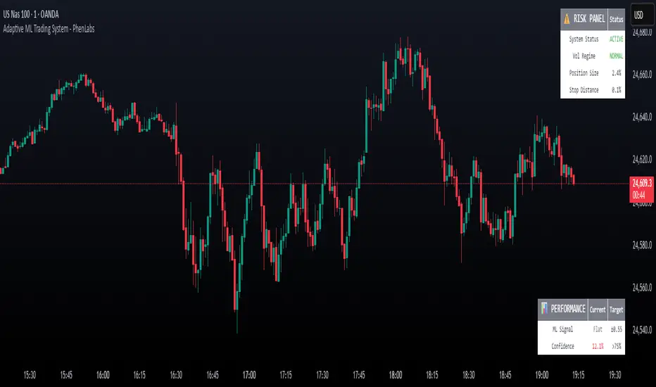
Adaptive Machine Learning Trading System [PhenLabs]📊Adaptive ML Trading System
Version: PineScript™v6
📌Description
The Adaptive ML Trading System is a sophisticated machine learning indicator that combines ensemble modeling with advanced technical analysis. This system uses XGBoost, Random Forest, and Neural Network algorithms to generate high-confidence trading signals while incorporating robust risk management features. Traders benefit from objective, data-driven decision-making that adapts to changing market conditions.
🚀Points of Innovation
• Machine Learning Ensemble - Three integrated models (XGBoost, Random Forest, Neural Network)
• Confidence-Based Trading - Only executes trades when ML confidence exceeds threshold
• Dynamic Risk Management - ATR-based stop loss and max drawdown protection
• Adaptive Position Sizing - Volatility-adjusted position sizing with confidence weighting
• Real-Time Performance Metrics - Live tracking of win rate, Sharpe ratio, and performance
• Multi-Timeframe Feature Analysis - Adaptive lookback periods for different market regimes
🔧Core Components
• ML Ensemble Engine - Weighted combination of XGBoost, Random Forest, and Neural Network outputs
• Feature Normalization System - Advanced preprocessing with custom tanh/sigmoid activation
• Risk Management Module - Dynamic position sizing and drawdown protection
• Performance Dashboard - Real-time metrics and risk status monitoring
• Alert System - Comprehensive alert conditions for entries, exits, and risk events
🔥Key Features
• High-confidence ML signals with customizable confidence thresholds
• Multiple trading modes (Conservative, Balanced, Aggressive) for different risk profiles
• Integrated stop loss and risk management with ATR-based calculations
• Real-time performance metrics including win rate and Sharpe ratio
• Comprehensive alert system with entry, exit, and risk management notifications
• Visual confidence bands and threshold indicators for easy signal interpretation
🎨Visualization
• ML Signal Line - Primary signal output ranging from -1 to +1
• Confidence Bands - Visual representation of model confidence levels
• Threshold Lines - Customizable buy/sell threshold levels
• Position Histogram - Current market position visualization
• Performance Tables - Real-time metrics display in customizable positions
📖Usage Guidelines
Model Configuration
• Confidence Threshold: Default 0.55, Range 0.5-0.95 - Minimum confidence for signals
• Model Sensitivity: Default 0.9, Range 0.1-2.0 - Adjusts signal sensitivity
• Ensemble Mode: Conservative/Balanced/Aggressive - Trading style preference
• Signal Threshold: Default 0.55, Range 0.3-0.9 - ML signal threshold for entries
Risk Management
• Position Size %: Default 10%, Range 1-50% - Portfolio percentage per trade
• Max Drawdown %: Default 15%, Range 5-30% - Maximum allowed drawdown
• Stop Loss ATR: Default 2.0, Range 0.5-5.0 - Stop loss in ATR multiples
• Dynamic Sizing: Default true - Volatility-based position adjustment
Display Settings
• Show Signals: Default true - Display entry/exit signals
• Show Threshold Signals: Default true - Display ±0.6 threshold crosses
• Show Confidence Bands: Default true - Display ML confidence levels
• Performance Dashboard: Default true - Show metrics table
✅Best Use Cases
• Swing trading with 1-5 day holding periods
• Trend-following strategies in established trends
• Volatility breakout trading during high-confidence periods
• Risk-adjusted position sizing for portfolio management
• Multi-timeframe confirmation for existing strategies
⚠️Limitations
• Requires sufficient historical data for accurate ML predictions
• May experience low confidence periods in choppy markets
• Performance varies across different asset classes and timeframes
• Not suitable for very short-term scalping strategies
• Requires understanding of basic risk management principles
💡What Makes This Unique
• True machine learning ensemble with multiple model types
• Confidence-based trading rather than simple signal generation
• Integrated risk management with dynamic position sizing
• Real-time performance tracking and metrics
• Adaptive parameters that adjust to market conditions
🔬How It Works
Feature Calculation: Computes 20+ technical features from price/volume data
Feature Normalization: Applies custom normalization for ML compatibility
Ensemble Prediction: Combines XGBoost, Random Forest, and Neural Network outputs
Signal Generation: Produces confidence-weighted trading signals
Risk Management: Applies position sizing and stop loss rules
Execution: Generates alerts and visual signals based on thresholds
💡Note:
This indicator works best on daily and 4-hour timeframes for most assets. Ensure you understand the risk management settings before live trading. The system includes automatic risk-off modes that halt trading during excessive drawdown periods.
Institutional Levels (CNN) - [PhenLabs]📊Institutional Levels (Convolutional Neural Network-inspired)
Version : PineScript™v6
📌Description
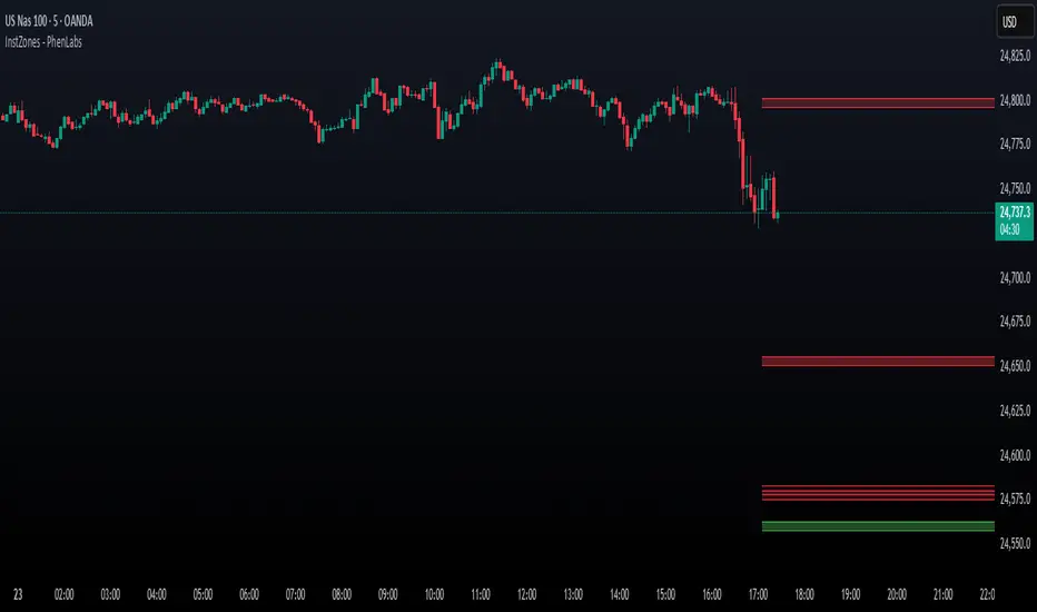
The CNN-IL Institutional Levels indicator represents a breakthrough in automated zone detection technology, combining convolutional neural network principles with advanced statistical modeling. This sophisticated tool identifies high-probability institutional trading zones by analyzing pivot patterns, volume dynamics, and price behavior using machine learning algorithms.
The indicator employs a proprietary 9-factor logistic regression model that calculates real-time reaction probabilities for each detected zone. By incorporating CNN-inspired filtering techniques and dynamic zone management, it provides traders with unprecedented accuracy in identifying where institutional money is likely to react to price action.
🚀Points of Innovation
● CNN-Inspired Pivot Analysis - Advanced binning system using convolutional neural network principles for superior pattern recognition
● Real-Time Probability Engine - Live reaction probability calculations using 9-factor logistic regression model
● Dynamic Zone Intelligence - Automatic zone merging using Intersection over Union (IoU) algorithms
● Volume-Weighted Scoring - Time-of-day volume Z-score analysis for enhanced zone strength assessment
● Adaptive Decay System - Intelligent zone lifecycle management based on touch frequency and recency
● Multi-Filter Architecture - Optional gradient, smoothing, and Difference of Gaussians (DoG) convolution filters
🔧Core Components
● Pivot Detection Engine - Advanced pivot identification with configurable left/right bars and ATR-normalized strength calculations
● Neural Network Binning - Price level clustering using CNN-inspired algorithms with ATR-based bin sizing
● Logistic Regression Model - 9-factor probability calculation including distance, width, volume, VWAP deviation, and trend analysis
● Zone Management System - Intelligent creation, merging, and decay algorithms for optimal zone lifecycle control
● Visualization Layer - Dynamic line drawing with opacity-based scoring and optional zone fills
🔥Key Features
● High-Probability Zone Detection - Automatically identifies institutional levels with reaction probabilities above configurable thresholds
● Real-Time Probability Scoring - Live calculation of zone reaction likelihood using advanced statistical modeling
● Session-Aware Analysis - Optional filtering to specific trading sessions for enhanced accuracy during active market hours
● Customizable Parameters - Full control over lookback periods, zone sensitivity, merge thresholds, and probability models
● Performance Optimized - Efficient processing with controlled update frequencies and pivot processing limits
● Non-Repainting Mode - Strict mode available for backtesting accuracy and live trading reliability
🎨Visualization
● Dynamic Zone Lines - Color-coded support and resistance levels with opacity reflecting zone strength and confidence scores
● Probability Labels - Real-time display of reaction probabilities, touch counts, and historical hit rates for active zones
● Zone Fills - Optional semi-transparent zone highlighting for enhanced visual clarity and immediate pattern recognition
● Adaptive Styling - Automatic color and opacity adjustments based on zone scoring and statistical significance
📖Usage Guidelines
● Lookback Bars - Default 500, Range 100-1000, Controls the historical data window for pivot analysis and zone calculation
● Pivot Left/Right - Default 3, Range 1-10, Defines the pivot detection sensitivity and confirmation requirements
● Bin Size ATR units - Default 0.25, Range 0.1-2.0, Controls price level clustering granularity for zone creation
● Base Zone Half-Width ATR units - Default 0.25, Range 0.1-1.0, Sets the minimum zone width in ATR units for institutional level boundaries
● Zone Merge IoU Threshold - Default 0.5, Range 0.1-0.9, Intersection over Union threshold for automatic zone merging algorithms
● Max Active Zones - Default 5, Range 3-20, Maximum number of zones displayed simultaneously to prevent chart clutter
● Probability Threshold for Labels - Default 0.6, Range 0.3-0.9, Minimum reaction probability required for zone label display and alerts
● Distance Weight w1 - Controls influence of price distance from zone center on reaction probability
● Width Weight w2 - Adjusts impact of zone width on probability calculations
● Volume Weight w3 - Modifies volume Z-score influence on zone strength assessment
● VWAP Weight w4 - Controls VWAP deviation impact on institutional level significance
● Touch Count Weight w5 - Adjusts influence of historical zone interactions on probability scoring
● Hit Rate Weight w6 - Controls prior success rate impact on future reaction likelihood predictions
● Wick Penetration Weight w7 - Modifies wick penetration analysis influence on probability calculations
● Trend Weight w8 - Adjusts trend context impact using ADX analysis for directional bias assessment
✅Best Use Cases
● Swing Trading Entries - Enter positions at high-probability institutional zones with 60%+ reaction scores
● Scalping Opportunities - Quick entries and exits around frequently tested institutional levels
● Risk Management - Use zones as dynamic stop-loss and take-profit levels based on institutional behavior
● Market Structure Analysis - Identify key institutional levels that define current market structure and sentiment
● Confluence Trading - Combine with other technical indicators for high-probability trade setups
● Session-Based Strategies - Focus analysis during high-volume sessions for maximum effectiveness
⚠️Limitations
● Historical Pattern Dependency - Algorithm effectiveness relies on historical patterns that may not repeat in changing market conditions
● Computational Intensity - Complex calculations may impact chart performance on lower-end devices or with multiple indicators
● Probability Estimates - Reaction probabilities are statistical estimates and do not guarantee actual market outcomes
● Session Sensitivity - Performance may vary significantly between different market sessions and volatility regimes
● Parameter Sensitivity - Results can be highly dependent on input parameters requiring optimization for different instruments
💡What Makes This Unique
● CNN Architecture - First indicator to apply convolutional neural network principles to institutional-level detection
● Real-Time ML Scoring - Live machine learning probability calculations for each zone interaction
● Advanced Zone Management - Sophisticated algorithms for zone lifecycle management and automatic optimization
● Statistical Rigor - Comprehensive 9-factor logistic regression model with extensive backtesting validation
● Performance Optimization - Efficient processing algorithms designed for real-time trading applications
🔬How It Works
● Multi-timeframe pivot identification - Uses configurable sensitivity parameters for advanced pivot detection
● ATR-normalized strength calculations - Standardizes pivot significance across different volatility regimes
● Volume Z-score integration - Enhanced pivot weighting based on time-of-day volume patterns
● Price level clustering - Neural network binning algorithms with ATR-based sizing for zone creation
● Recency decay applications - Weights recent pivots more heavily than historical data for relevance
● Statistical filtering - Eliminates low-significance price levels and reduces market noise
● Dynamic zone generation - Creates zones from statistically significant pivot clusters with minimum support thresholds
● IoU-based merging algorithms - Combines overlapping zones while maintaining accuracy using Intersection over Union
● Adaptive decay systems - Automatic removal of outdated or low-performing zones for optimal performance
● 9-factor logistic regression - Incorporates distance, width, volume, VWAP, touch history, and trend analysis
● Real-time scoring updates - Zone interaction calculations with configurable threshold filtering
● Optional CNN filters - Gradient detection, smoothing, and Difference of Gaussians processing for enhanced accuracy
💡Note
This indicator represents advanced quantitative analysis and should be used by traders familiar with statistical modeling concepts. The probability scores are mathematical estimates based on historical patterns and should be combined with proper risk management and additional technical analysis for optimal trading decisions.
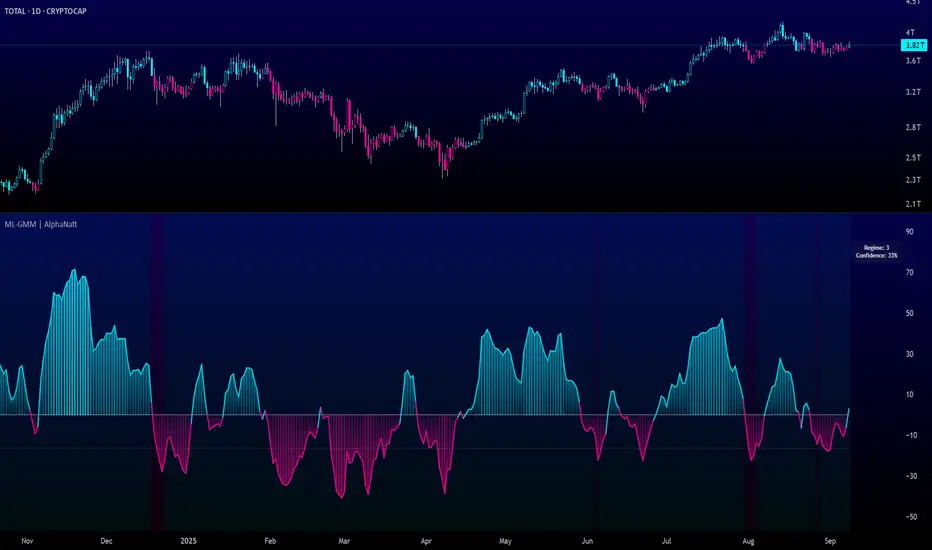
Machine Learning Gaussian Mixture Model | AlphaNattMachine Learning Gaussian Mixture Model | AlphaNatt
A revolutionary oscillator that uses Gaussian Mixture Models (GMM) with unsupervised machine learning to identify market regimes and automatically adapt momentum calculations - bringing statistical pattern recognition techniques to trading.
"Markets don't follow a single distribution - they're a mixture of different regimes. This oscillator identifies which regime we're in and adapts accordingly."
━━━━━━━━━━━━━━━━━━━━━━━━━━━━━━━━━━━━━━━━
🤖 THE MACHINE LEARNING
Gaussian Mixture Models (GMM):
Unlike K-means clustering which assigns hard boundaries, GMM uses probabilistic clustering :
Models data as coming from multiple Gaussian distributions
Each market regime is a different Gaussian component
Provides probability of belonging to each regime
More sophisticated than simple clustering
Expectation-Maximization Algorithm:
The indicator continuously learns and adapts using the E-M algorithm:
E-step: Calculate probability of current market belonging to each regime
M-step: Update regime parameters based on new data
Continuous learning without repainting
Adapts to changing market conditions
━━━━━━━━━━━━━━━━━━━━━━━━━━━━━━━━━━━━━━━━
🎯 THREE MARKET REGIMES
The GMM identifies three distinct market states:
Regime 1 - Low Volatility:
Quiet, ranging markets
Uses RSI-based momentum calculation
Reduces false signals in choppy conditions
Background: Pink tint
Regime 2 - Normal Market:
Standard trending conditions
Uses Rate of Change momentum
Balanced sensitivity
Background: Gray tint
Regime 3 - High Volatility:
Strong trends or volatility events
Uses Z-score based momentum
Captures extreme moves
Background: Cyan tint
━━━━━━━━━━━━━━━━━━━━━━━━━━━━━━━━━━━━━━━━
💡 KEY INNOVATIONS
1. Probabilistic Regime Detection:
Instead of binary regime assignment, provides probabilities:
30% Regime 1, 60% Regime 2, 10% Regime 3
Smooth transitions between regimes
No sudden indicator jumps
2. Weighted Momentum Calculation:
Combines three different momentum formulas
Weights based on regime probabilities
Automatically adapts to market conditions
3. Confidence Indicator:
Shows how certain the model is (white line)
High confidence = strong regime identification
Low confidence = transitional market state
Line transparency changes with confidence
━━━━━━━━━━━━━━━━━━━━━━━━━━━━━━━━━━━━━━━━
⚙️ PARAMETER OPTIMIZATION
Training Period (50-500):
50-100: Quick adaptation to recent conditions
100: Balanced (default)
200-500: Stable regime identification
Number of Components (2-5):
2: Simple bull/bear regimes
3: Low/Normal/High volatility (default)
4-5: More granular regime detection
Learning Rate (0.1-1.0):
0.1-0.3: Slow, stable learning
0.3: Balanced (default)
0.5-1.0: Fast adaptation
━━━━━━━━━━━━━━━━━━━━━━━━━━━━━━━━━━━━━━━━
📊 TRADING STRATEGIES
Visual Signals:
Cyan gradient: Bullish momentum
Magenta gradient: Bearish momentum
Background color: Current regime
Confidence line: Model certainty
1. Regime-Based Trading:
Regime 1 (pink): Expect mean reversion
Regime 2 (gray): Standard trend following
Regime 3 (cyan): Strong momentum trades
2. Confidence-Filtered Signals:
Only trade when confidence > 70%
High confidence = clearer market state
Avoid transitions (low confidence)
3. Adaptive Position Sizing:
Regime 1: Smaller positions (choppy)
Regime 2: Normal positions
Regime 3: Larger positions (trending)
━━━━━━━━━━━━━━━━━━━━━━━━━━━━━━━━━━━━━━━━
🚀 ADVANTAGES OVER OTHER ML INDICATORS
vs K-Means Clustering:
Soft clustering (probabilities) vs hard boundaries
Captures uncertainty and transitions
More mathematically robust
vs KNN (K-Nearest Neighbors):
Unsupervised learning (no historical labels needed)
Continuous adaptation
Lower computational complexity
vs Neural Networks:
Interpretable (know what each regime means)
No overfitting issues
Works with limited data
━━━━━━━━━━━━━━━━━━━━━━━━━━━━━━━━━━━━━━━━
📈 PERFORMANCE CHARACTERISTICS
Best Market Conditions:
Markets with clear regime shifts
Volatile to trending transitions
Multi-timeframe analysis
Cryptocurrency markets (high regime variation)
Key Strengths:
Automatically adapts to market changes
No manual parameter adjustment needed
Smooth transitions between regimes
Probabilistic confidence measure
━━━━━━━━━━━━━━━━━━━━━━━━━━━━━━━━━━━━━━━━
🔬 TECHNICAL BACKGROUND
Gaussian Mixture Models are used extensively in:
Speech recognition (Google Assistant)
Computer vision (facial recognition)
Astronomy (galaxy classification)
Genomics (gene expression analysis)
Finance (risk modeling at investment banks)
The E-M algorithm was developed at Stanford in 1977 and is one of the most important algorithms in unsupervised machine learning.
━━━━━━━━━━━━━━━━━━━━━━━━━━━━━━━━━━━━━━━━
💡 PRO TIPS
Watch regime transitions: Best opportunities often occur when regimes change
Combine with volume: High volume + regime change = strong signal
Use confidence filter: Avoid low confidence periods
Multi-timeframe: Compare regimes across timeframes
Adjust position size: Scale based on identified regime
━━━━━━━━━━━━━━━━━━━━━━━━━━━━━━━━━━━━━━━━
⚠️ IMPORTANT NOTES
Machine learning adapts but doesn't predict the future
Best used with other confirmation indicators
Allow time for model to learn (100+ bars)
Not financial advice - educational purposes
Backtest thoroughly on your instruments
━━━━━━━━━━━━━━━━━━━━━━━━━━━━━━━━━━━━━━━━
🏆 CONCLUSION
The GMM Momentum Oscillator brings institutional-grade machine learning to retail trading. By identifying market regimes probabilistically and adapting momentum calculations accordingly, it provides:
Automatic adaptation to market conditions
Clear regime identification with confidence levels
Smooth, professional signal generation
True unsupervised machine learning
This isn't just another indicator with "ML" in the name - it's a genuine implementation of Gaussian Mixture Models with the Expectation-Maximization algorithm, the same technology used in:
Google's speech recognition
Tesla's computer vision
NASA's data analysis
Wall Street risk models
"Let the machine learn the market regimes. Trade with statistical confidence."
━━━━━━━━━━━━━━━━━━━━━━━━━━━━━━━━━━━━━━━━
Developed by AlphaNatt | Machine Learning Trading Systems
Version: 1.0
Algorithm: Gaussian Mixture Model with E-M
Classification: Unsupervised Learning Oscillator
Not financial advice. Always DYOR.
AI-Weighted RSI (Zeiierman)█ Overview
AI-Weighted RSI (Zeiierman) is an adaptive oscillator that enhances classic RSI by applying a correlation-weighted prediction layer. Instead of looking only at RSI values directly, this indicator continuously evaluates how other price- and volume-based features (returns, volatility, volume shifts) correlate with RSI, and then weights them accordingly to project the next RSI state.
The result is a smoother, forward-looking RSI framework that adapts to market conditions in real time.
By leveraging feature correlation instead of static formulas, AI-Weighted RSI behaves like a lightweight learning model, adjusting its emphasis depending on which features are most aligned with RSI behavior during the current regime.
█ How It Works
⚪ Feature Extraction
Each bar, the script computes features: log returns, RSI itself, ATR% (volatility), volume, and volume log-change.
⚪ Correlation Screening
Over a rolling learning window, it measures the correlation of each feature against RSI. The strongest relationships are ranked and selected.
⚪ Adaptive Weighting
Features are standardized (z-scored), then combined using their signed correlations as weights, building a rolling, adaptive prediction of RSI.
⚪ Prediction to RSI Weight
The predicted RSI is mapped back into a “weight” scale (±2 by default). Above 0 = bullish bias, below 0 = bearish bias, with color-graded fills to visualize overbought/oversold pressure.
⚪ Signal Line
A smoothing option (signal length) overlays a moving average of the AI-Weighted RSI for clearer trend confirmation.
█ Why AI-Weighted RSI
⚪ Adaptive to Market Regime
Because the model re-evaluates correlations continuously, it naturally shifts which features dominate, sometimes volatility explains RSI best, sometimes volume, sometimes returns.
⚪ Forward-Looking Bias
Instead of simply reflecting RSI, the model provides a projection, helping anticipate shifts in momentum before RSI itself flips.
█ How to Use
⚪ Directional Bias
Read the RSI relative to 0. Above = bullish momentum bias, below = bearish.
⚪ Overbought / Oversold Zones
Shaded fills beyond +0.5 or -0.5 highlight extremes where RSI pressure often exhausts.
⚪ Divergences
When price makes new highs/lows but AI-Weighted RSI fails to confirm, it often signals weakening momentum.
█ Settings
RSI Length: Lookback for the core RSI calculation.
Signal Length: Smoothing applied to the AI-Weighted RSI output.
Learning Window: Bars used for correlation learning and z-scoring.
-----------------
Disclaimer
The content provided in my scripts, indicators, ideas, algorithms, and systems is for educational and informational purposes only. It does not constitute financial advice, investment recommendations, or a solicitation to buy or sell any financial instruments. I will not accept liability for any loss or damage, including without limitation any loss of profit, which may arise directly or indirectly from the use of or reliance on such information.
All investments involve risk, and the past performance of a security, industry, sector, market, financial product, trading strategy, backtest, or individual's trading does not guarantee future results or returns. Investors are fully responsible for any investment decisions they make. Such decisions should be based solely on an evaluation of their financial circumstances, investment objectives, risk tolerance, and liquidity needs.

Machine Learning-Inspired Supply & Demand Zones [AlgoPoint]This indicator is a Smart Supply & Demand Zone tool, developed with principles inspired by Machine Learning (ML). It intelligently filters out market noise, allowing you to focus only on the most significant zones where institutional order flow is likely present.
💡 How It Works: Why Is This Indicator "Smart"?
Unlike traditional indicators that only measure simple price movements, this script uses an algorithm that asks the same critical questions an experienced market analyst would to qualify a zone:
- 1. Price Imbalance: How fast and aggressively did the price leave the zone? Our algorithm measures the body size of the "departure candle" relative to the current market volatility (ATR). A zone is only considered if it was formed by an explosive move that is statistically significant, indicating a major imbalance between buyers and sellers.
- 2. Volume Confirmation: Did the "smart money" participate in this move? The script checks if the volume on the departure candle was significantly higher than the recent average volume. A spike in volume confirms that the move was backed by institutional interest, adding strength and validity to the zone.
- 3. Valid Pivot Structure: Did the zone originate from a meaningful swing high or low? The algorithm first identifies a valid pivot structure, ensuring that zones are not drawn from insignificant or random price fluctuations.
Only when a potential zone passes these three critical tests—our "quality filter"—is it drawn on your chart.
🚀 Features & How to Use
Using the indicator is straightforward. You will see two primary types of boxes on your chart:
* 🟥 Red Box (Supply Zone): An area of potential resistance where selling pressure is likely to be strong. Look for potential shorting opportunities as the price approaches this zone.
* 🟩 Green Box (Demand Zone): An area of potential support where buying pressure is likely to be strong. Look for potential long opportunities as the price pulls back into this zone.
Dynamic Zone Management
This indicator is not static; it lives and breathes with the market:
- Fresh Zone: A newly formed zone appears in its full, vibrant color. These are the highest-probability zones as they have not yet been re-tested.
- Broken / Flipped Zone: You have full control over what happens when a zone is broken! In the settings, you can choose:
- Delete Zone: The zone will be removed completely when the price closes through it.
- Show as Broken (Flip): When broken, the zone will turn gray, stop extending, and remain on your chart. This is extremely useful for identifying Support/Resistance Flips, where a broken demand zone becomes new resistance, or a broken supply zone becomes new support.
⚙️ Settings & Customization
Fine-tune the indicator to match your personal trading style via the settings menu:
- Breakout Behavior: The most powerful feature. Choose between Delete Zone and Show as Broken (Flip) to customize your chart.
- Zone Finding Logic: Control the indicator's sensitivity.
- Selective: Requires both strong imbalance and high volume. Finds fewer, but higher-quality, zones.
- Moderate: Requires either strong imbalance or high volume. Finds more potential zones.
- Sensitivity Settings: Adjust the ATR Multiplier and Volume Multiplier to make the criteria for a "strong" zone stricter or looser.
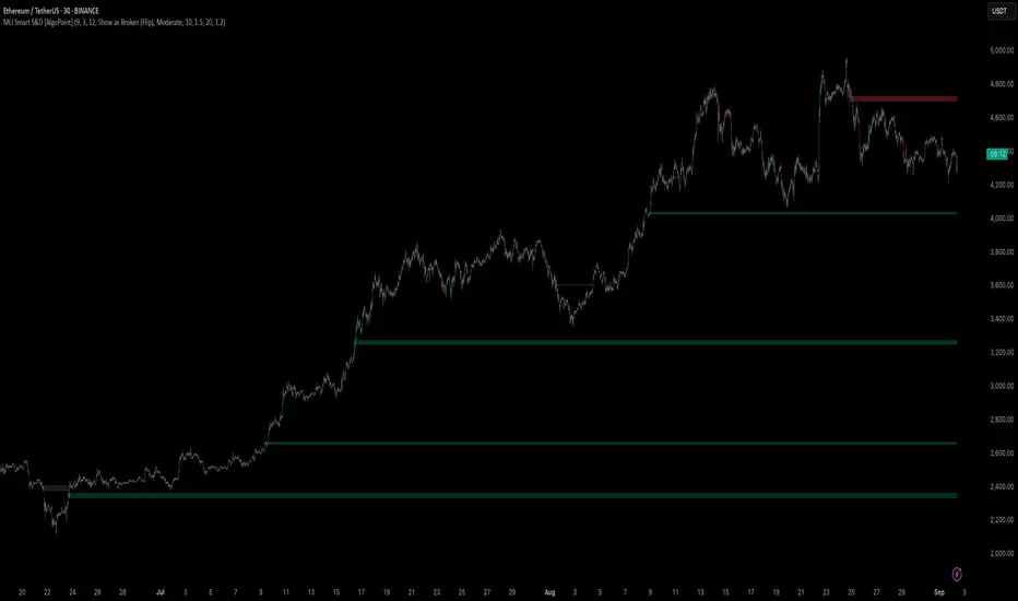
Machine Learning BBPct [BackQuant]Machine Learning BBPct
What this is (in one line)
A Bollinger Band %B oscillator enhanced with a simplified K-Nearest Neighbors (KNN) pattern matcher. The model compares today’s context (volatility, momentum, volume, and position inside the bands) to similar situations in recent history and blends that historical consensus back into the raw %B to reduce noise and improve context awareness. It is informational and diagnostic—designed to describe market state, not to sell a trading system.
Background: %B in plain terms
Bollinger %B measures where price sits inside its dynamic envelope: 0 at the lower band, 1 at the upper band, ~ 0.5 near the basis (the moving average). Readings toward 1 indicate pressure near the envelope’s upper edge (often strength or stretch), while readings toward 0 indicate pressure near the lower edge (often weakness or stretch). Because bands adapt to volatility, %B is naturally comparable across regimes.
Why add (simplified) KNN?
Classic %B is reactive and can be whippy in fast regimes. The simplified KNN layer builds a “nearest-neighbor memory” of recent market states and asks: “When the market looked like this before, where did %B tend to be next bar?” It then blends that estimate with the current %B. Key ideas:
• Feature vector . Each bar is summarized by up to five normalized features:
– %B itself (normalized)
– Band width (volatility proxy)
– Price momentum (ROC)
– Volume momentum (ROC of volume)
– Price position within the bands
• Distance metric . Euclidean distance ranks the most similar recent bars.
• Prediction . Average the neighbors’ prior %B (lagged to avoid lookahead), inverse-weighted by distance.
• Blend . Linearly combine raw %B and KNN-predicted %B with a configurable weight; optional filtering then adapts to confidence.
This remains “simplified” KNN: no training/validation split, no KD-trees, no scaling beyond windowed min-max, and no probabilistic calibration.
How the script is organized (by input groups)
1) BBPct Settings
• Price Source – Which price to evaluate (%B is computed from this).
• Calculation Period – Lookback for SMA basis and standard deviation.
• Multiplier – Standard deviation width (e.g., 2.0).
• Apply Smoothing / Type / Length – Optional smoothing of the %B stream before ML (EMA, RMA, DEMA, TEMA, LINREG, HMA, etc.). Turning this off gives you the raw %B.
2) Thresholds
• Overbought/Oversold – Default 0.8 / 0.2 (inside ).
• Extreme OB/OS – Stricter zones (e.g., 0.95 / 0.05) to flag stretch conditions.
3) KNN Machine Learning
• Enable KNN – Switch between pure %B and hybrid.
• K (neighbors) – How many historical analogs to blend (default 8).
• Historical Period – Size of the search window for neighbors.
• ML Weight – Blend between raw %B and KNN estimate.
• Number of Features – Use 2–5 features; higher counts add context but raise the risk of overfitting in short windows.
4) Filtering
• Method – None, Adaptive, Kalman-style (first-order),
or Hull smoothing.
• Strength – How aggressively to smooth. “Adaptive” uses model confidence to modulate its alpha: higher confidence → stronger reliance on the ML estimate.
5) Performance Tracking
• Win-rate Period – Simple running score of past signal outcomes based on target/stop/time-out logic (informational, not a robust backtest).
• Early Entry Lookback – Horizon for forecasting a potential threshold cross.
• Profit Target / Stop Loss – Used only by the internal win-rate heuristic.
6) Self-Optimization
• Enable Self-Optimization – Lightweight, rolling comparison of a few canned settings (K = 8/14/21 via simple rules on %B extremes).
• Optimization Window & Stability Threshold – Governs how quickly preferred K changes and how sensitive the overfitting alarm is.
• Adaptive Thresholds – Adjust the OB/OS lines with volatility regime (ATR ratio), widening in calm markets and tightening in turbulent ones (bounded 0.7–0.9 and 0.1–0.3).
7) UI Settings
• Show Table / Zones / ML Prediction / Early Signals – Toggle informational overlays.
• Signal Line Width, Candle Painting, Colors – Visual preferences.
Step-by-step logic
A) Compute %B
Basis = SMA(source, len); dev = stdev(source, len) × multiplier; Upper/Lower = Basis ± dev.
%B = (price − Lower) / (Upper − Lower). Optional smoothing yields standardBB .
B) Build the feature vector
All features are min-max normalized over the KNN window so distances are in comparable units. Features include normalized %B, normalized band width, normalized price ROC, normalized volume ROC, and normalized position within bands. You can limit to the first N features (2–5).
C) Find nearest neighbors
For each bar inside the lookback window, compute the Euclidean distance between current features and that bar’s features. Sort by distance, keep the top K .
D) Predict and blend
Use inverse-distance weights (with a strong cap for near-zero distances) to average neighbors’ prior %B (lagged by one bar). This becomes the KNN estimate. Blend it with raw %B via the ML weight. A variance of neighbor %B around the prediction becomes an uncertainty proxy ; combined with a stability score (how long parameters remain unchanged), it forms mlConfidence ∈ . The Adaptive filter optionally transforms that confidence into a smoothing coefficient.
E) Adaptive thresholds
Volatility regime (ATR(14) divided by its 50-bar SMA) nudges OB/OS thresholds wider or narrower within fixed bounds. The aim: comparable extremeness across regimes.
F) Early entry heuristic
A tiny two-step slope/acceleration probe extrapolates finalBB forward a few bars. If it is on track to cross OB/OS soon (and slope/acceleration agree), it flags an EARLY_BUY/SELL candidate with an internal confidence score. This is explicitly a heuristic—use as an attention cue, not a signal by itself.
G) Informational win-rate
The script keeps a rolling array of trade outcomes derived from signal transitions + rudimentary exits (target/stop/time). The percentage shown is a rough diagnostic , not a validated backtest.
Outputs and visual language
• ML Bollinger %B (finalBB) – The main line after KNN blending and optional filtering.
• Gradient fill – Greenish tones above 0.5, reddish below, with intensity following distance from the midline.
• Adaptive zones – Overbought/oversold and extreme bands; shaded backgrounds appear at extremes.
• ML Prediction (dots) – The KNN estimate plotted as faint circles; becomes bright white when confidence > 0.7.
• Early arrows – Optional small triangles for approaching OB/OS.
• Candle painting – Light green above the midline, light red below (optional).
• Info panel – Current value, signal classification, ML confidence, optimized K, stability, volatility regime, adaptive thresholds, overfitting flag, early-entry status, and total signals processed.
Signal classification (informational)
The indicator does not fire trade commands; it labels state:
• STRONG_BUY / STRONG_SELL – finalBB beyond extreme OS/OB thresholds.
• BUY / SELL – finalBB beyond adaptive OS/OB.
• EARLY_BUY / EARLY_SELL – forecast suggests a near-term cross with decent internal confidence.
• NEUTRAL – between adaptive bands.
Alerts (what you can automate)
• Entering adaptive OB/OS and extreme OB/OS.
• Midline cross (0.5).
• Overfitting detected (frequent parameter flipping).
• Early signals when early confidence > 0.7.
These are purely descriptive triggers around the indicator’s state.
Practical interpretation
• Mean-reversion context – In range markets, adaptive OS/OB with ML smoothing can reduce whipsaws relative to raw %B.
• Trend context – In persistent trends, the KNN blend can keep finalBB nearer the mid/upper region during healthy pullbacks if history supports similar contexts.
• Regime awareness – Watch the volatility regime and adaptive thresholds. If thresholds compress (high vol), “OB/OS” comes sooner; if thresholds widen (calm), it takes more stretch to flag.
• Confidence as a weight – High mlConfidence implies neighbors agree; you may rely more on the ML curve. Low confidence argues for de-emphasizing ML and leaning on raw %B or other tools.
• Stability score – Rising stability indicates consistent parameter selection and fewer flips; dropping stability hints at a shifting backdrop.
Methodological notes
• Normalization uses rolling min-max over the KNN window. This is simple and scale-agnostic but sensitive to outliers; the distance metric will reflect that.
• Distance is unweighted Euclidean. If you raise featureCount, you increase dimensionality; consider keeping K larger and lookback ample to avoid sparse-neighbor artifacts.
• Lag handling intentionally uses neighbors’ previous %B for prediction to avoid lookahead bias.
• Self-optimization is deliberately modest: it only compares a few canned K/threshold choices using simple “did an extreme anticipate movement?” scoring, then enforces a stability regime and an overfitting guard. It is not a grid search or GA.
• Kalman option is a first-order recursive filter (fixed gain), not a full state-space estimator.
• Hull option derives a dynamic length from 1/strength; it is a convenience smoothing alternative.
Limitations and cautions
• Non-stationarity – Nearest neighbors from the recent window may not represent the future under structural breaks (policy shifts, liquidity shocks).
• Curse of dimensionality – Adding features without sufficient lookback can make genuine neighbors rare.
• Overfitting risk – The script includes a crude overfitting detector (frequent parameter flips) and will fall back to defaults when triggered, but this is only a guardrail.
• Win-rate display – The internal score is illustrative; it does not constitute a tradable backtest.
• Latency vs. smoothness – Smoothing and ML blending reduce noise but add lag; tune to your timeframe and objectives.
Tuning guide
• Short-term scalping – Lower len (10–14), slightly lower multiplier (1.8–2.0), small K (5–8), featureCount 3–4, Adaptive filter ON, moderate strength.
• Swing trading – len (20–30), multiplier ~2.0, K (8–14), featureCount 4–5, Adaptive thresholds ON, filter modest.
• Strong trends – Consider higher adaptive_upper/lower bounds (or let volatility regime do it), keep ML weight moderate so raw %B still reflects surges.
• Chop – Higher ML weight and stronger Adaptive filtering; accept lag in exchange for fewer false extremes.
How to use it responsibly
Treat this as a state descriptor and context filter. Pair it with your execution signals (structure breaks, volume footprints, higher-timeframe bias) and risk management. If mlConfidence is low or stability is falling, lean less on the ML line and more on raw %B or external confirmation.
Summary
Machine Learning BBPct augments a familiar oscillator with a transparent, simplified KNN memory of recent conditions. By blending neighbors’ behavior into %B and adapting thresholds to volatility regime—while exposing confidence, stability, and a plain early-entry heuristic—it provides an informational, probability-minded view of stretch and reversion that you can interpret alongside your own process.
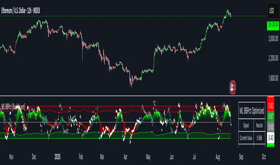
Markov Chain [3D] | FractalystWhat exactly is a Markov Chain?
This indicator uses a Markov Chain model to analyze, quantify, and visualize the transitions between market regimes (Bull, Bear, Neutral) on your chart. It dynamically detects these regimes in real-time, calculates transition probabilities, and displays them as animated 3D spheres and arrows, giving traders intuitive insight into current and future market conditions.
How does a Markov Chain work, and how should I read this spheres-and-arrows diagram?
Think of three weather modes: Sunny, Rainy, Cloudy.
Each sphere is one mode. The loop on a sphere means “stay the same next step” (e.g., Sunny again tomorrow).
The arrows leaving a sphere show where things usually go next if they change (e.g., Sunny moving to Cloudy).
Some paths matter more than others. A more prominent loop means the current mode tends to persist. A more prominent outgoing arrow means a change to that destination is the usual next step.
Direction isn’t symmetric: moving Sunny→Cloudy can behave differently than Cloudy→Sunny.
Now relabel the spheres to markets: Bull, Bear, Neutral.
Spheres: market regimes (uptrend, downtrend, range).
Self‑loop: tendency for the current regime to continue on the next bar.
Arrows: the most common next regime if a switch happens.
How to read: Start at the sphere that matches current bar state. If the loop stands out, expect continuation. If one outgoing path stands out, that switch is the typical next step. Opposite directions can differ (Bear→Neutral doesn’t have to match Neutral→Bear).
What states and transitions are shown?
The three market states visualized are:
Bullish (Bull): Upward or strong-market regime.
Bearish (Bear): Downward or weak-market regime.
Neutral: Sideways or range-bound regime.
Bidirectional animated arrows and probability labels show how likely the market is to move from one regime to another (e.g., Bull → Bear or Neutral → Bull).
How does the regime detection system work?
You can use either built-in price returns (based on adaptive Z-score normalization) or supply three custom indicators (such as volume, oscillators, etc.).
Values are statistically normalized (Z-scored) over a configurable lookback period.
The normalized outputs are classified into Bull, Bear, or Neutral zones.
If using three indicators, their regime signals are averaged and smoothed for robustness.
How are transition probabilities calculated?
On every confirmed bar, the algorithm tracks the sequence of detected market states, then builds a rolling window of transitions.
The code maintains a transition count matrix for all regime pairs (e.g., Bull → Bear).
Transition probabilities are extracted for each possible state change using Laplace smoothing for numerical stability, and frequently updated in real-time.
What is unique about the visualization?
3D animated spheres represent each regime and change visually when active.
Animated, bidirectional arrows reveal transition probabilities and allow you to see both dominant and less likely regime flows.
Particles (moving dots) animate along the arrows, enhancing the perception of regime flow direction and speed.
All elements dynamically update with each new price bar, providing a live market map in an intuitive, engaging format.
Can I use custom indicators for regime classification?
Yes! Enable the "Custom Indicators" switch and select any three chart series as inputs. These will be normalized and combined (each with equal weight), broadening the regime classification beyond just price-based movement.
What does the “Lookback Period” control?
Lookback Period (default: 100) sets how much historical data builds the probability matrix. Shorter periods adapt faster to regime changes but may be noisier. Longer periods are more stable but slower to adapt.
How is this different from a Hidden Markov Model (HMM)?
It sets the window for both regime detection and probability calculations. Lower values make the system more reactive, but potentially noisier. Higher values smooth estimates and make the system more robust.
How is this Markov Chain different from a Hidden Markov Model (HMM)?
Markov Chain (as here): All market regimes (Bull, Bear, Neutral) are directly observable on the chart. The transition matrix is built from actual detected regimes, keeping the model simple and interpretable.
Hidden Markov Model: The actual regimes are unobservable ("hidden") and must be inferred from market output or indicator "emissions" using statistical learning algorithms. HMMs are more complex, can capture more subtle structure, but are harder to visualize and require additional machine learning steps for training.
A standard Markov Chain models transitions between observable states using a simple transition matrix, while a Hidden Markov Model assumes the true states are hidden (latent) and must be inferred from observable “emissions” like price or volume data. In practical terms, a Markov Chain is transparent and easier to implement and interpret; an HMM is more expressive but requires statistical inference to estimate hidden states from data.
Markov Chain: states are observable; you directly count or estimate transition probabilities between visible states. This makes it simpler, faster, and easier to validate and tune.
HMM: states are hidden; you only observe emissions generated by those latent states. Learning involves machine learning/statistical algorithms (commonly Baum–Welch/EM for training and Viterbi for decoding) to infer both the transition dynamics and the most likely hidden state sequence from data.
How does the indicator avoid “repainting” or look-ahead bias?
All regime changes and matrix updates happen only on confirmed (closed) bars, so no future data is leaked, ensuring reliable real-time operation.
Are there practical tuning tips?
Tune the Lookback Period for your asset/timeframe: shorter for fast markets, longer for stability.
Use custom indicators if your asset has unique regime drivers.
Watch for rapid changes in transition probabilities as early warning of a possible regime shift.
Who is this indicator for?
Quants and quantitative researchers exploring probabilistic market modeling, especially those interested in regime-switching dynamics and Markov models.
Programmers and system developers who need a probabilistic regime filter for systematic and algorithmic backtesting:
The Markov Chain indicator is ideally suited for programmatic integration via its bias output (1 = Bull, 0 = Neutral, -1 = Bear).
Although the visualization is engaging, the core output is designed for automated, rules-based workflows—not for discretionary/manual trading decisions.
Developers can connect the indicator’s output directly to their Pine Script logic (using input.source()), allowing rapid and robust backtesting of regime-based strategies.
It acts as a plug-and-play regime filter: simply plug the bias output into your entry/exit logic, and you have a scientifically robust, probabilistically-derived signal for filtering, timing, position sizing, or risk regimes.
The MC's output is intentionally "trinary" (1/0/-1), focusing on clear regime states for unambiguous decision-making in code. If you require nuanced, multi-probability or soft-label state vectors, consider expanding the indicator or stacking it with a probability-weighted logic layer in your scripting.
Because it avoids subjectivity, this approach is optimal for systematic quants, algo developers building backtested, repeatable strategies based on probabilistic regime analysis.
What's the mathematical foundation behind this?
The mathematical foundation behind this Markov Chain indicator—and probabilistic regime detection in finance—draws from two principal models: the (standard) Markov Chain and the Hidden Markov Model (HMM).
How to use this indicator programmatically?
The Markov Chain indicator automatically exports a bias value (+1 for Bullish, -1 for Bearish, 0 for Neutral) as a plot visible in the Data Window. This allows you to integrate its regime signal into your own scripts and strategies for backtesting, automation, or live trading.
Step-by-Step Integration with Pine Script (input.source)
Add the Markov Chain indicator to your chart.
This must be done first, since your custom script will "pull" the bias signal from the indicator's plot.
In your strategy, create an input using input.source()
Example:
//@version=5
strategy("MC Bias Strategy Example")
mcBias = input.source(close, "MC Bias Source")
After saving, go to your script’s settings. For the “MC Bias Source” input, select the plot/output of the Markov Chain indicator (typically its bias plot).
Use the bias in your trading logic
Example (long only on Bull, flat otherwise):
if mcBias == 1
strategy.entry("Long", strategy.long)
else
strategy.close("Long")
For more advanced workflows, combine mcBias with additional filters or trailing stops.
How does this work behind-the-scenes?
TradingView’s input.source() lets you use any plot from another indicator as a real-time, “live” data feed in your own script (source).
The selected bias signal is available to your Pine code as a variable, enabling logical decisions based on regime (trend-following, mean-reversion, etc.).
This enables powerful strategy modularity : decouple regime detection from entry/exit logic, allowing fast experimentation without rewriting core signal code.
Integrating 45+ Indicators with Your Markov Chain — How & Why
The Enhanced Custom Indicators Export script exports a massive suite of over 45 technical indicators—ranging from classic momentum (RSI, MACD, Stochastic, etc.) to trend, volume, volatility, and oscillator tools—all pre-calculated, centered/scaled, and available as plots.
// Enhanced Custom Indicators Export - 45 Technical Indicators
// Comprehensive technical analysis suite for advanced market regime detection
//@version=6
indicator('Enhanced Custom Indicators Export | Fractalyst', shorttitle='Enhanced CI Export', overlay=false, scale=scale.right, max_labels_count=500, max_lines_count=500)
// |----- Input Parameters -----| //
momentum_group = "Momentum Indicators"
trend_group = "Trend Indicators"
volume_group = "Volume Indicators"
volatility_group = "Volatility Indicators"
oscillator_group = "Oscillator Indicators"
display_group = "Display Settings"
// Common lengths
length_14 = input.int(14, "Standard Length (14)", minval=1, maxval=100, group=momentum_group)
length_20 = input.int(20, "Medium Length (20)", minval=1, maxval=200, group=trend_group)
length_50 = input.int(50, "Long Length (50)", minval=1, maxval=200, group=trend_group)
// Display options
show_table = input.bool(true, "Show Values Table", group=display_group)
table_size = input.string("Small", "Table Size", options= , group=display_group)
// |----- MOMENTUM INDICATORS (15 indicators) -----| //
// 1. RSI (Relative Strength Index)
rsi_14 = ta.rsi(close, length_14)
rsi_centered = rsi_14 - 50
// 2. Stochastic Oscillator
stoch_k = ta.stoch(close, high, low, length_14)
stoch_d = ta.sma(stoch_k, 3)
stoch_centered = stoch_k - 50
// 3. Williams %R
williams_r = ta.stoch(close, high, low, length_14) - 100
// 4. MACD (Moving Average Convergence Divergence)
= ta.macd(close, 12, 26, 9)
// 5. Momentum (Rate of Change)
momentum = ta.mom(close, length_14)
momentum_pct = (momentum / close ) * 100
// 6. Rate of Change (ROC)
roc = ta.roc(close, length_14)
// 7. Commodity Channel Index (CCI)
cci = ta.cci(close, length_20)
// 8. Money Flow Index (MFI)
mfi = ta.mfi(close, length_14)
mfi_centered = mfi - 50
// 9. Awesome Oscillator (AO)
ao = ta.sma(hl2, 5) - ta.sma(hl2, 34)
// 10. Accelerator Oscillator (AC)
ac = ao - ta.sma(ao, 5)
// 11. Chande Momentum Oscillator (CMO)
cmo = ta.cmo(close, length_14)
// 12. Detrended Price Oscillator (DPO)
dpo = close - ta.sma(close, length_20)
// 13. Price Oscillator (PPO)
ppo = ta.sma(close, 12) - ta.sma(close, 26)
ppo_pct = (ppo / ta.sma(close, 26)) * 100
// 14. TRIX
trix_ema1 = ta.ema(close, length_14)
trix_ema2 = ta.ema(trix_ema1, length_14)
trix_ema3 = ta.ema(trix_ema2, length_14)
trix = ta.roc(trix_ema3, 1) * 10000
// 15. Klinger Oscillator
klinger = ta.ema(volume * (high + low + close) / 3, 34) - ta.ema(volume * (high + low + close) / 3, 55)
// 16. Fisher Transform
fisher_hl2 = 0.5 * (hl2 - ta.lowest(hl2, 10)) / (ta.highest(hl2, 10) - ta.lowest(hl2, 10)) - 0.25
fisher = 0.5 * math.log((1 + fisher_hl2) / (1 - fisher_hl2))
// 17. Stochastic RSI
stoch_rsi = ta.stoch(rsi_14, rsi_14, rsi_14, length_14)
stoch_rsi_centered = stoch_rsi - 50
// 18. Relative Vigor Index (RVI)
rvi_num = ta.swma(close - open)
rvi_den = ta.swma(high - low)
rvi = rvi_den != 0 ? rvi_num / rvi_den : 0
// 19. Balance of Power (BOP)
bop = (close - open) / (high - low)
// |----- TREND INDICATORS (10 indicators) -----| //
// 20. Simple Moving Average Momentum
sma_20 = ta.sma(close, length_20)
sma_momentum = ((close - sma_20) / sma_20) * 100
// 21. Exponential Moving Average Momentum
ema_20 = ta.ema(close, length_20)
ema_momentum = ((close - ema_20) / ema_20) * 100
// 22. Parabolic SAR
sar = ta.sar(0.02, 0.02, 0.2)
sar_trend = close > sar ? 1 : -1
// 23. Linear Regression Slope
lr_slope = ta.linreg(close, length_20, 0) - ta.linreg(close, length_20, 1)
// 24. Moving Average Convergence (MAC)
mac = ta.sma(close, 10) - ta.sma(close, 30)
// 25. Trend Intensity Index (TII)
tii_sum = 0.0
for i = 1 to length_20
tii_sum += close > close ? 1 : 0
tii = (tii_sum / length_20) * 100
// 26. Ichimoku Cloud Components
ichimoku_tenkan = (ta.highest(high, 9) + ta.lowest(low, 9)) / 2
ichimoku_kijun = (ta.highest(high, 26) + ta.lowest(low, 26)) / 2
ichimoku_signal = ichimoku_tenkan > ichimoku_kijun ? 1 : -1
// 27. MESA Adaptive Moving Average (MAMA)
mama_alpha = 2.0 / (length_20 + 1)
mama = ta.ema(close, length_20)
mama_momentum = ((close - mama) / mama) * 100
// 28. Zero Lag Exponential Moving Average (ZLEMA)
zlema_lag = math.round((length_20 - 1) / 2)
zlema_data = close + (close - close )
zlema = ta.ema(zlema_data, length_20)
zlema_momentum = ((close - zlema) / zlema) * 100
// |----- VOLUME INDICATORS (6 indicators) -----| //
// 29. On-Balance Volume (OBV)
obv = ta.obv
// 30. Volume Rate of Change (VROC)
vroc = ta.roc(volume, length_14)
// 31. Price Volume Trend (PVT)
pvt = ta.pvt
// 32. Negative Volume Index (NVI)
nvi = 0.0
nvi := volume < volume ? nvi + ((close - close ) / close ) * nvi : nvi
// 33. Positive Volume Index (PVI)
pvi = 0.0
pvi := volume > volume ? pvi + ((close - close ) / close ) * pvi : pvi
// 34. Volume Oscillator
vol_osc = ta.sma(volume, 5) - ta.sma(volume, 10)
// 35. Ease of Movement (EOM)
eom_distance = high - low
eom_box_height = volume / 1000000
eom = eom_box_height != 0 ? eom_distance / eom_box_height : 0
eom_sma = ta.sma(eom, length_14)
// 36. Force Index
force_index = volume * (close - close )
force_index_sma = ta.sma(force_index, length_14)
// |----- VOLATILITY INDICATORS (10 indicators) -----| //
// 37. Average True Range (ATR)
atr = ta.atr(length_14)
atr_pct = (atr / close) * 100
// 38. Bollinger Bands Position
bb_basis = ta.sma(close, length_20)
bb_dev = 2.0 * ta.stdev(close, length_20)
bb_upper = bb_basis + bb_dev
bb_lower = bb_basis - bb_dev
bb_position = bb_dev != 0 ? (close - bb_basis) / bb_dev : 0
bb_width = bb_dev != 0 ? (bb_upper - bb_lower) / bb_basis * 100 : 0
// 39. Keltner Channels Position
kc_basis = ta.ema(close, length_20)
kc_range = ta.ema(ta.tr, length_20)
kc_upper = kc_basis + (2.0 * kc_range)
kc_lower = kc_basis - (2.0 * kc_range)
kc_position = kc_range != 0 ? (close - kc_basis) / kc_range : 0
// 40. Donchian Channels Position
dc_upper = ta.highest(high, length_20)
dc_lower = ta.lowest(low, length_20)
dc_basis = (dc_upper + dc_lower) / 2
dc_position = (dc_upper - dc_lower) != 0 ? (close - dc_basis) / (dc_upper - dc_lower) : 0
// 41. Standard Deviation
std_dev = ta.stdev(close, length_20)
std_dev_pct = (std_dev / close) * 100
// 42. Relative Volatility Index (RVI)
rvi_up = ta.stdev(close > close ? close : 0, length_14)
rvi_down = ta.stdev(close < close ? close : 0, length_14)
rvi_total = rvi_up + rvi_down
rvi_volatility = rvi_total != 0 ? (rvi_up / rvi_total) * 100 : 50
// 43. Historical Volatility
hv_returns = math.log(close / close )
hv = ta.stdev(hv_returns, length_20) * math.sqrt(252) * 100
// 44. Garman-Klass Volatility
gk_vol = math.log(high/low) * math.log(high/low) - (2*math.log(2)-1) * math.log(close/open) * math.log(close/open)
gk_volatility = math.sqrt(ta.sma(gk_vol, length_20)) * 100
// 45. Parkinson Volatility
park_vol = math.log(high/low) * math.log(high/low)
parkinson = math.sqrt(ta.sma(park_vol, length_20) / (4 * math.log(2))) * 100
// 46. Rogers-Satchell Volatility
rs_vol = math.log(high/close) * math.log(high/open) + math.log(low/close) * math.log(low/open)
rogers_satchell = math.sqrt(ta.sma(rs_vol, length_20)) * 100
// |----- OSCILLATOR INDICATORS (5 indicators) -----| //
// 47. Elder Ray Index
elder_bull = high - ta.ema(close, 13)
elder_bear = low - ta.ema(close, 13)
elder_power = elder_bull + elder_bear
// 48. Schaff Trend Cycle (STC)
stc_macd = ta.ema(close, 23) - ta.ema(close, 50)
stc_k = ta.stoch(stc_macd, stc_macd, stc_macd, 10)
stc_d = ta.ema(stc_k, 3)
stc = ta.stoch(stc_d, stc_d, stc_d, 10)
// 49. Coppock Curve
coppock_roc1 = ta.roc(close, 14)
coppock_roc2 = ta.roc(close, 11)
coppock = ta.wma(coppock_roc1 + coppock_roc2, 10)
// 50. Know Sure Thing (KST)
kst_roc1 = ta.roc(close, 10)
kst_roc2 = ta.roc(close, 15)
kst_roc3 = ta.roc(close, 20)
kst_roc4 = ta.roc(close, 30)
kst = ta.sma(kst_roc1, 10) + 2*ta.sma(kst_roc2, 10) + 3*ta.sma(kst_roc3, 10) + 4*ta.sma(kst_roc4, 15)
// 51. Percentage Price Oscillator (PPO)
ppo_line = ((ta.ema(close, 12) - ta.ema(close, 26)) / ta.ema(close, 26)) * 100
ppo_signal = ta.ema(ppo_line, 9)
ppo_histogram = ppo_line - ppo_signal
// |----- PLOT MAIN INDICATORS -----| //
// Plot key momentum indicators
plot(rsi_centered, title="01_RSI_Centered", color=color.purple, linewidth=1)
plot(stoch_centered, title="02_Stoch_Centered", color=color.blue, linewidth=1)
plot(williams_r, title="03_Williams_R", color=color.red, linewidth=1)
plot(macd_histogram, title="04_MACD_Histogram", color=color.orange, linewidth=1)
plot(cci, title="05_CCI", color=color.green, linewidth=1)
// Plot trend indicators
plot(sma_momentum, title="06_SMA_Momentum", color=color.navy, linewidth=1)
plot(ema_momentum, title="07_EMA_Momentum", color=color.maroon, linewidth=1)
plot(sar_trend, title="08_SAR_Trend", color=color.teal, linewidth=1)
plot(lr_slope, title="09_LR_Slope", color=color.lime, linewidth=1)
plot(mac, title="10_MAC", color=color.fuchsia, linewidth=1)
// Plot volatility indicators
plot(atr_pct, title="11_ATR_Pct", color=color.yellow, linewidth=1)
plot(bb_position, title="12_BB_Position", color=color.aqua, linewidth=1)
plot(kc_position, title="13_KC_Position", color=color.olive, linewidth=1)
plot(std_dev_pct, title="14_StdDev_Pct", color=color.silver, linewidth=1)
plot(bb_width, title="15_BB_Width", color=color.gray, linewidth=1)
// Plot volume indicators
plot(vroc, title="16_VROC", color=color.blue, linewidth=1)
plot(eom_sma, title="17_EOM", color=color.red, linewidth=1)
plot(vol_osc, title="18_Vol_Osc", color=color.green, linewidth=1)
plot(force_index_sma, title="19_Force_Index", color=color.orange, linewidth=1)
plot(obv, title="20_OBV", color=color.purple, linewidth=1)
// Plot additional oscillators
plot(ao, title="21_Awesome_Osc", color=color.navy, linewidth=1)
plot(cmo, title="22_CMO", color=color.maroon, linewidth=1)
plot(dpo, title="23_DPO", color=color.teal, linewidth=1)
plot(trix, title="24_TRIX", color=color.lime, linewidth=1)
plot(fisher, title="25_Fisher", color=color.fuchsia, linewidth=1)
// Plot more momentum indicators
plot(mfi_centered, title="26_MFI_Centered", color=color.yellow, linewidth=1)
plot(ac, title="27_AC", color=color.aqua, linewidth=1)
plot(ppo_pct, title="28_PPO_Pct", color=color.olive, linewidth=1)
plot(stoch_rsi_centered, title="29_StochRSI_Centered", color=color.silver, linewidth=1)
plot(klinger, title="30_Klinger", color=color.gray, linewidth=1)
// Plot trend continuation
plot(tii, title="31_TII", color=color.blue, linewidth=1)
plot(ichimoku_signal, title="32_Ichimoku_Signal", color=color.red, linewidth=1)
plot(mama_momentum, title="33_MAMA_Momentum", color=color.green, linewidth=1)
plot(zlema_momentum, title="34_ZLEMA_Momentum", color=color.orange, linewidth=1)
plot(bop, title="35_BOP", color=color.purple, linewidth=1)
// Plot volume continuation
plot(nvi, title="36_NVI", color=color.navy, linewidth=1)
plot(pvi, title="37_PVI", color=color.maroon, linewidth=1)
plot(momentum_pct, title="38_Momentum_Pct", color=color.teal, linewidth=1)
plot(roc, title="39_ROC", color=color.lime, linewidth=1)
plot(rvi, title="40_RVI", color=color.fuchsia, linewidth=1)
// Plot volatility continuation
plot(dc_position, title="41_DC_Position", color=color.yellow, linewidth=1)
plot(rvi_volatility, title="42_RVI_Volatility", color=color.aqua, linewidth=1)
plot(hv, title="43_Historical_Vol", color=color.olive, linewidth=1)
plot(gk_volatility, title="44_GK_Volatility", color=color.silver, linewidth=1)
plot(parkinson, title="45_Parkinson_Vol", color=color.gray, linewidth=1)
// Plot final oscillators
plot(rogers_satchell, title="46_RS_Volatility", color=color.blue, linewidth=1)
plot(elder_power, title="47_Elder_Power", color=color.red, linewidth=1)
plot(stc, title="48_STC", color=color.green, linewidth=1)
plot(coppock, title="49_Coppock", color=color.orange, linewidth=1)
plot(kst, title="50_KST", color=color.purple, linewidth=1)
// Plot final indicators
plot(ppo_histogram, title="51_PPO_Histogram", color=color.navy, linewidth=1)
plot(pvt, title="52_PVT", color=color.maroon, linewidth=1)
// |----- Reference Lines -----| //
hline(0, "Zero Line", color=color.gray, linestyle=hline.style_dashed, linewidth=1)
hline(50, "Midline", color=color.gray, linestyle=hline.style_dotted, linewidth=1)
hline(-50, "Lower Midline", color=color.gray, linestyle=hline.style_dotted, linewidth=1)
hline(25, "Upper Threshold", color=color.gray, linestyle=hline.style_dotted, linewidth=1)
hline(-25, "Lower Threshold", color=color.gray, linestyle=hline.style_dotted, linewidth=1)
// |----- Enhanced Information Table -----| //
if show_table and barstate.islast
table_position = position.top_right
table_text_size = table_size == "Tiny" ? size.tiny : table_size == "Small" ? size.small : size.normal
var table info_table = table.new(table_position, 3, 18, bgcolor=color.new(color.white, 85), border_width=1, border_color=color.gray)
// Headers
table.cell(info_table, 0, 0, 'Category', text_color=color.black, text_size=table_text_size, bgcolor=color.new(color.blue, 70))
table.cell(info_table, 1, 0, 'Indicator', text_color=color.black, text_size=table_text_size, bgcolor=color.new(color.blue, 70))
table.cell(info_table, 2, 0, 'Value', text_color=color.black, text_size=table_text_size, bgcolor=color.new(color.blue, 70))
// Key Momentum Indicators
table.cell(info_table, 0, 1, 'MOMENTUM', text_color=color.purple, text_size=table_text_size, bgcolor=color.new(color.purple, 90))
table.cell(info_table, 1, 1, 'RSI Centered', text_color=color.purple, text_size=table_text_size)
table.cell(info_table, 2, 1, str.tostring(rsi_centered, '0.00'), text_color=color.purple, text_size=table_text_size)
table.cell(info_table, 0, 2, '', text_color=color.blue, text_size=table_text_size)
table.cell(info_table, 1, 2, 'Stoch Centered', text_color=color.blue, text_size=table_text_size)
table.cell(info_table, 2, 2, str.tostring(stoch_centered, '0.00'), text_color=color.blue, text_size=table_text_size)
table.cell(info_table, 0, 3, '', text_color=color.red, text_size=table_text_size)
table.cell(info_table, 1, 3, 'Williams %R', text_color=color.red, text_size=table_text_size)
table.cell(info_table, 2, 3, str.tostring(williams_r, '0.00'), text_color=color.red, text_size=table_text_size)
table.cell(info_table, 0, 4, '', text_color=color.orange, text_size=table_text_size)
table.cell(info_table, 1, 4, 'MACD Histogram', text_color=color.orange, text_size=table_text_size)
table.cell(info_table, 2, 4, str.tostring(macd_histogram, '0.000'), text_color=color.orange, text_size=table_text_size)
table.cell(info_table, 0, 5, '', text_color=color.green, text_size=table_text_size)
table.cell(info_table, 1, 5, 'CCI', text_color=color.green, text_size=table_text_size)
table.cell(info_table, 2, 5, str.tostring(cci, '0.00'), text_color=color.green, text_size=table_text_size)
// Key Trend Indicators
table.cell(info_table, 0, 6, 'TREND', text_color=color.navy, text_size=table_text_size, bgcolor=color.new(color.navy, 90))
table.cell(info_table, 1, 6, 'SMA Momentum %', text_color=color.navy, text_size=table_text_size)
table.cell(info_table, 2, 6, str.tostring(sma_momentum, '0.00'), text_color=color.navy, text_size=table_text_size)
table.cell(info_table, 0, 7, '', text_color=color.maroon, text_size=table_text_size)
table.cell(info_table, 1, 7, 'EMA Momentum %', text_color=color.maroon, text_size=table_text_size)
table.cell(info_table, 2, 7, str.tostring(ema_momentum, '0.00'), text_color=color.maroon, text_size=table_text_size)
table.cell(info_table, 0, 8, '', text_color=color.teal, text_size=table_text_size)
table.cell(info_table, 1, 8, 'SAR Trend', text_color=color.teal, text_size=table_text_size)
table.cell(info_table, 2, 8, str.tostring(sar_trend, '0'), text_color=color.teal, text_size=table_text_size)
table.cell(info_table, 0, 9, '', text_color=color.lime, text_size=table_text_size)
table.cell(info_table, 1, 9, 'Linear Regression', text_color=color.lime, text_size=table_text_size)
table.cell(info_table, 2, 9, str.tostring(lr_slope, '0.000'), text_color=color.lime, text_size=table_text_size)
// Key Volatility Indicators
table.cell(info_table, 0, 10, 'VOLATILITY', text_color=color.yellow, text_size=table_text_size, bgcolor=color.new(color.yellow, 90))
table.cell(info_table, 1, 10, 'ATR %', text_color=color.yellow, text_size=table_text_size)
table.cell(info_table, 2, 10, str.tostring(atr_pct, '0.00'), text_color=color.yellow, text_size=table_text_size)
table.cell(info_table, 0, 11, '', text_color=color.aqua, text_size=table_text_size)
table.cell(info_table, 1, 11, 'BB Position', text_color=color.aqua, text_size=table_text_size)
table.cell(info_table, 2, 11, str.tostring(bb_position, '0.00'), text_color=color.aqua, text_size=table_text_size)
table.cell(info_table, 0, 12, '', text_color=color.olive, text_size=table_text_size)
table.cell(info_table, 1, 12, 'KC Position', text_color=color.olive, text_size=table_text_size)
table.cell(info_table, 2, 12, str.tostring(kc_position, '0.00'), text_color=color.olive, text_size=table_text_size)
// Key Volume Indicators
table.cell(info_table, 0, 13, 'VOLUME', text_color=color.blue, text_size=table_text_size, bgcolor=color.new(color.blue, 90))
table.cell(info_table, 1, 13, 'Volume ROC', text_color=color.blue, text_size=table_text_size)
table.cell(info_table, 2, 13, str.tostring(vroc, '0.00'), text_color=color.blue, text_size=table_text_size)
table.cell(info_table, 0, 14, '', text_color=color.red, text_size=table_text_size)
table.cell(info_table, 1, 14, 'EOM', text_color=color.red, text_size=table_text_size)
table.cell(info_table, 2, 14, str.tostring(eom_sma, '0.000'), text_color=color.red, text_size=table_text_size)
// Key Oscillators
table.cell(info_table, 0, 15, 'OSCILLATORS', text_color=color.purple, text_size=table_text_size, bgcolor=color.new(color.purple, 90))
table.cell(info_table, 1, 15, 'Awesome Osc', text_color=color.blue, text_size=table_text_size)
table.cell(info_table, 2, 15, str.tostring(ao, '0.000'), text_color=color.blue, text_size=table_text_size)
table.cell(info_table, 0, 16, '', text_color=color.red, text_size=table_text_size)
table.cell(info_table, 1, 16, 'Fisher Transform', text_color=color.red, text_size=table_text_size)
table.cell(info_table, 2, 16, str.tostring(fisher, '0.000'), text_color=color.red, text_size=table_text_size)
// Summary Statistics
table.cell(info_table, 0, 17, 'SUMMARY', text_color=color.black, text_size=table_text_size, bgcolor=color.new(color.gray, 70))
table.cell(info_table, 1, 17, 'Total Indicators: 52', text_color=color.black, text_size=table_text_size)
regime_color = rsi_centered > 10 ? color.green : rsi_centered < -10 ? color.red : color.gray
regime_text = rsi_centered > 10 ? "BULLISH" : rsi_centered < -10 ? "BEARISH" : "NEUTRAL"
table.cell(info_table, 2, 17, regime_text, text_color=regime_color, text_size=table_text_size)
This makes it the perfect “indicator backbone” for quantitative and systematic traders who want to prototype, combine, and test new regime detection models—especially in combination with the Markov Chain indicator.
How to use this script with the Markov Chain for research and backtesting:
Add the Enhanced Indicator Export to your chart.
Every calculated indicator is available as an individual data stream.
Connect the indicator(s) you want as custom input(s) to the Markov Chain’s “Custom Indicators” option.
In the Markov Chain indicator’s settings, turn ON the custom indicator mode.
For each of the three custom indicator inputs, select the exported plot from the Enhanced Export script—the menu lists all 45+ signals by name.
This creates a powerful, modular regime-detection engine where you can mix-and-match momentum, trend, volume, or custom combinations for advanced filtering.
Backtest regime logic directly.
Once you’ve connected your chosen indicators, the Markov Chain script performs regime detection (Bull/Neutral/Bear) based on your selected features—not just price returns.
The regime detection is robust, automatically normalized (using Z-score), and outputs bias (1, -1, 0) for plug-and-play integration.
Export the regime bias for programmatic use.
As described above, use input.source() in your Pine Script strategy or system and link the bias output.
You can now filter signals, control trade direction/size, or design pairs-trading that respect true, indicator-driven market regimes.
With this framework, you’re not limited to static or simplistic regime filters. You can rigorously define, test, and refine what “market regime” means for your strategies—using the technical features that matter most to you.
Optimize your signal generation by backtesting across a universe of meaningful indicator blends.
Enhance risk management with objective, real-time regime boundaries.
Accelerate your research: iterate quickly, swap indicator components, and see results with minimal code changes.
Automate multi-asset or pairs-trading by integrating regime context directly into strategy logic.
Add both scripts to your chart, connect your preferred features, and start investigating your best regime-based trades—entirely within the TradingView ecosystem.
References & Further Reading
Ang, A., & Bekaert, G. (2002). “Regime Switches in Interest Rates.” Journal of Business & Economic Statistics, 20(2), 163–182.
Hamilton, J. D. (1989). “A New Approach to the Economic Analysis of Nonstationary Time Series and the Business Cycle.” Econometrica, 57(2), 357–384.
Markov, A. A. (1906). "Extension of the Limit Theorems of Probability Theory to a Sum of Variables Connected in a Chain." The Notes of the Imperial Academy of Sciences of St. Petersburg.
Guidolin, M., & Timmermann, A. (2007). “Asset Allocation under Multivariate Regime Switching.” Journal of Economic Dynamics and Control, 31(11), 3503–3544.
Murphy, J. J. (1999). Technical Analysis of the Financial Markets. New York Institute of Finance.
Brock, W., Lakonishok, J., & LeBaron, B. (1992). “Simple Technical Trading Rules and the Stochastic Properties of Stock Returns.” Journal of Finance, 47(5), 1731–1764.
Zucchini, W., MacDonald, I. L., & Langrock, R. (2017). Hidden Markov Models for Time Series: An Introduction Using R (2nd ed.). Chapman and Hall/CRC.
On Quantitative Finance and Markov Models:
Lo, A. W., & Hasanhodzic, J. (2009). The Heretics of Finance: Conversations with Leading Practitioners of Technical Analysis. Bloomberg Press.
Patterson, S. (2016). The Man Who Solved the Market: How Jim Simons Launched the Quant Revolution. Penguin Press.
TradingView Pine Script Documentation: www.tradingview.com
TradingView Blog: “Use an Input From Another Indicator With Your Strategy” www.tradingview.com
GeeksforGeeks: “What is the Difference Between Markov Chains and Hidden Markov Models?” www.geeksforgeeks.org
What makes this indicator original and unique?
- On‑chart, real‑time Markov. The chain is drawn directly on your chart. You see the current regime, its tendency to stay (self‑loop), and the usual next step (arrows) as bars confirm.
- Source‑agnostic by design. The engine runs on any series you select via input.source() — price, your own oscillator, a composite score, anything you compute in the script.
- Automatic normalization + regime mapping. Different inputs live on different scales. The script standardizes your chosen source and maps it into clear regimes (e.g., Bull / Bear / Neutral) without you micromanaging thresholds each time.
- Rolling, bar‑by‑bar learning. Transition tendencies are computed from a rolling window of confirmed bars. What you see is exactly what the market did in that window.
- Fast experimentation. Switch the source, adjust the window, and the Markov view updates instantly. It’s a rapid way to test ideas and feel regime persistence/switch behavior.
Integrate your own signals (using input.source())
- In settings, choose the Source . This is powered by input.source() .
- Feed it price, an indicator you compute inside the script, or a custom composite series.
- The script will automatically normalize that series and process it through the Markov engine, mapping it to regimes and updating the on‑chart spheres/arrows in real time.
Credits:
Deep gratitude to @RicardoSantos for both the foundational Markov chain processing engine and inspiring open-source contributions, which made advanced probabilistic market modeling accessible to the TradingView community.
Special thanks to @Alien_Algorithms for the innovative and visually stunning 3D sphere logic that powers the indicator’s animated, regime-based visualization.
Disclaimer
This tool summarizes recent behavior. It is not financial advice and not a guarantee of future results.

Correlation HeatMap [TradingFinder] Sessions Data Science Stats🔵 Introduction
n financial markets, correlation describes the statistical relationship between the price movements of two assets and how they interact over time. It plays a key role in both trading and investing by helping analyze asset behavior, manage portfolio risk, and understand intermarket dynamics. The Correlation Heatmap is a visual tool that shows how the correlation between multiple assets and a central reference asset (the Main Symbol) changes over time.
It supports four market types forex, stocks, crypto, and a custom mode making it adaptable to different trading environments. The heatmap uses a color-coded grid where warmer tones represent stronger negative correlations and cooler tones indicate stronger positive ones. This intuitive color system allows traders to quickly identify when assets move together or diverge, offering real-time insights that go beyond traditional correlation tables.
🟣 How to Interpret the Heatmap Visually ?
Each cell represents the correlation between the main symbol and one compared asset at a specific time.
Warm colors (e.g. red, orange) suggest strong negative correlation as one asset rises, the other tends to fall.
Cool colors (e.g. blue, green) suggest strong positive correlation both assets tend to move in the same direction.
Lighter shades indicate weaker correlations, while darker shades indicate stronger correlations.
The heatmap updates over time, allowing users to detect changes in correlation during market events or trading sessions.
One of the standout features of this indicator is its ability to overlay global market sessions such as Tokyo, London, New York, or major equity opens directly onto the heatmap timeline. This alignment lets traders observe how correlation structures respond to real-world session changes. For example, they can spot when assets shift from being inversely correlated to moving together as a new session opens, potentially signaling new momentum or macro flow. The customizable symbol setup (including up to 20 compared assets) makes it ideal not only for forex and crypto traders but also for multi-asset and sector-based stock analysis.
🟣 Use Cases and Advantages
Analyze sector rotation in equities by tracking correlation to major indices like SPX or DJI.
Monitor altcoin behavior relative to Bitcoin to find early entry opportunities in crypto markets.
Detect changes in currency alignment with DXY across trading sessions in forex.
Identify correlation breakdowns during market volatility, signaling possible new trends.
Use correlation shifts as confirmation for trade setups or to hedge multi-asset exposure
🔵 How to Use
Correlation is one of the core concepts in financial analysis and allows traders to understand how assets behave in relation to one another. The Correlation Heatmap extends this idea by going beyond a simple number or static matrix. Instead, it presents a dynamic visual map of how correlations shift over time.
In this indicator, a Main Symbol is selected as the reference point for analysis. In standard modes such as forex, stocks, or crypto, the symbol currently shown on the main chart is automatically used as the main symbol. This allows users to begin correlation analysis right away without adjusting any settings.
The horizontal axis of the heatmap shows time, while the vertical axis lists the selected assets. Each cell on the heatmap shows the correlation between that asset and the main symbol at a given moment.
This approach is especially useful for intermarket analysis. In forex, for example, tracking how currency pairs like OANDA:EURUSD EURUSD, FX:GBPUSD GBPUSD, and PEPPERSTONE:AUDUSD AUDUSD correlate with TVC:DXY DXY can give insight into broader capital flow.
If these pairs start showing increasing positive correlation with DXY say, shifting from blue to light green it could signal the start of a new phase or reversal. Conversely, if negative correlation fades gradually, it may suggest weakening relationships and more independent or volatile movement.
In the crypto market, watching how altcoins correlate with Bitcoin can help identify ideal entry points in secondary assets. In the stock market, analyzing how companies within the same sector move in relation to a major index like SP:SPX SPX or DJ:DJI DJI is also a highly effective technique for both technical and fundamental analysts.
This indicator not only visualizes correlation but also displays major market sessions. When enabled, this feature helps traders observe how correlation behavior changes at the start of each session, whether it's Tokyo, London, New York, or the opening of stock exchanges. Many key shifts, breakouts, or reversals tend to happen around these times, and the heatmap makes them easy to spot.
Another important feature is the market selection mode. Users can switch between forex, crypto, stocks, or custom markets and see correlation behavior specific to each one. In custom mode, users can manually select any combination of symbols for more advanced or personalized analysis. This makes the heatmap valuable not only for forex traders but also for stock traders, crypto analysts, and multi-asset strategists.
Finally, the heatmap's color-coded design helps users make sense of the data quickly. Warm colors such as red and orange reflect stronger negative correlations, while cool colors like blue and green represent stronger positive relationships. This simplicity and clarity make the tool accessible to both beginners and experienced traders.
🔵 Settings
Correlation Period: Allows you to set how many historical bars are used for calculating correlation. A higher number means a smoother, slower-moving heatmap, while a lower number makes it more responsive to recent changes.
Select Market: Lets you choose between Forex, Stock, Crypto, or Custom. In the first three options, the chart’s active symbol is automatically used as the Main Symbol. In Custom mode, you can manually define the Main Symbol and up to 20 Compared Symbols.
Show Open Session: Enables the display of major trading sessions such as Tokyo, London, New York, or equity market opening hours directly on the timeline. This helps you connect correlation shifts with real-world market activity.
Market Mode: Lets you select whether the displayed sessions relate to the forex or stock market.
🔵 Conclusion
The Correlation Heatmap is a robust and flexible tool for analyzing the relationship between assets across different markets. By tracking how correlations change in real time, traders can better identify alignment or divergence between symbols and gain valuable insights into market structure.
Support for multiple asset classes, session overlays, and intuitive visual cues make this one of the most effective tools for intermarket analysis.
Whether you’re looking to manage portfolio risk, validate entry points, or simply understand capital flow across markets, this heatmap provides a clear and actionable perspective that you can rely on.

Smart Money Scalper v1 [Structure | VIDYA | Oscillator | Delta]🧠 What’s Included in the Core Module:
Component Description-
🔹 Trend Structure + Bias- Detect BoS/ChoCH from Lux-style logic to define bullish/bearish intent.
🟩 Key Level Mapping Structure- based support/resistance and smart money reaction zones.
🔺 VIDYA Slope Filter- Detects smart money accumulation via adaptive volume/trend shifts.
🔸 Two Pole Oscillator- Fast trend strength + direction change confirmation.
🧃 Delta Volume Pressure- Measures real buy/sell aggression (accumulation vs distribution).
🚫 No Trade Zone Logic- Triggers in low volatility, mixed signals, or structure uncertainty.
📊 Bias Labels & Arrows- Display directional bias, trade zones, and visual entries only when clear.
📈 What You’ll See on Chart-
- Key structure swing highs/lows.
- Bull/Bear bias labels (top left).
- Buy/Sell arrows only when all smart money confirmations align.
- Gray zones showing no-trade periods (chop, conflict, low delta).

Composite Trend Trader Module [BackQuant]Composite Trend Trader Module
Overview and Purpose
The Composite Trend Trader Module (CTM) is an invite-only Pine Script indicator designed to provide traders with a comprehensive tool for trend-following, dip-buying, and market strength assessment. By integrating multiple market data inputs—price momentum, volatility, volume, and statistical baselines—the CTM generates actionable outputs for trend identification, swing trade entries, and dip-buying opportunities. The indicator is intended for traders seeking a systematic approach to market analysis with customizable settings, while maintaining simplicity in its user interface. As a closed-source script, the underlying calculations remain proprietary, but this description outlines its functionality, features, and practical applications in trading.
Visual Components
The CTM provides the following visual elements on the chart:
• Signal Spine – A colored line (default 25-period weighted moving average) that reflects the dominant trend—green for bullish, red for bearish, and grey for neutral or transitional periods.
• Swing Triggers – Unicode markers ("𝕃" for long, "𝕊" for short) appear below or above bars when the trend shifts, signaling potential swing trade entries.
• Dip-Hunter Signals – Green arrows mark dip-buying opportunities, accompanied by faint green background highlights and forward-projecting entry lines for precise entry levels.
• Heat Meter – A horizontal strip at the bottom of the chart, graded from -50 (overheated) to +50 (deep dip), visually indicates the strength of dip conditions using a red-to-green gradient.
Core Features
The CTM comprises several components that work together to deliver a cohesive trading framework. Below is a detailed explanation of each, without disclosing proprietary calculations.
1. Universal Trend Tracking (UTT)
The UTT combines multiple momentum and statistical indicators into a single composite score ranging from -1 to +1. This score is derived from:
• Price-based momentum metrics.
• Volatility-adjusted thresholds.
• Statistical measures of price deviation and market structure.
When the UTT score exceeds +0.2, the market is considered in an actionable uptrend; below -0.2, a downtrend is identified. Values between these thresholds indicate a neutral or choppy market, helping traders avoid low-probability setups during consolidation.
2. Signal Spine
The signal spine is a 25-period weighted moving average of price, colored according to the UTT score (green for bullish, red for bearish, grey for neutral). This line serves as a visual anchor for tracking the prevailing trend and highlights regime changes in real time, enabling traders to align their strategies with market direction.
3. Swing Triggers (𝕃/𝕊)
Swing trade signals are generated when the UTT crosses the zero line, indicating a shift in market regime. A "𝕃" marker appears below the bar for a bullish crossover (potential long entry), and a "𝕊" marker appears above for a bearish crossover (potential short entry). These signals incorporate volatility-adaptive thresholds to minimize false triggers during low-volatility periods, improving reliability compared to traditional moving-average crossovers.
4. Dip-Hunter Engine
The Dip-Hunter subsystem identifies high-probability dip-buying opportunities by evaluating five conditions:
• Dip Magnitude – The price must have fallen by a user-defined percentage (default 2%) from a recent swing high, calculated over a specified lookback period (default 5 bars).
• Volume Burst – Current volume must exceed the average volume over a user-defined lookback (default 65 bars) by a specified multiplier (default 2x).
• Volatility Spike – The intraday range or Average True Range (ATR) must exceed a statistical baseline by a user-defined multiplier (default 1.5x).
• Structural Permission – Price must be below a fast Exponential Moving Average (EMA, default 20 periods), and the market structure must be bearish (fast EMA below slow EMA, default 50 periods).
• Trend Filter (Optional) – When enabled, dip signals are only generated if the UTT indicates a bullish trend, preventing trades against a bearish macro environment.
When these conditions align, the Dip-Hunter plots a green arrow, highlights the candle background, and draws a forward-projecting horizontal line at a user-selected price level (Low, Close, or calculated dip percentage).
5. Strength Score and Heat Meter
Each bar is assigned a strength score (0 to 5, or -50 to +50 when scaled for the heat meter) based on the following criteria:
• +1 for meeting the dip threshold.
• +1 for a volume spike.
• +1 for a volume momentum spike (based on rate-of-change).
• +1 for a confirmed volatility spike.
• +1 if price is below the fast EMA.
• +2 if the macro trend filter is bullish (when enabled).
The heat meter visualizes this score as a pointer on a red-to-green gradient strip, enabling traders to quickly assess the intensity of dip conditions and prioritize high-quality setups.
6. Entry-Line Generator
For each dip signal, the CTM draws a forward-projecting horizontal line to mark potential entry levels. Traders can configure:
• The price level for the line (Low, Close, or exact dip percentage).
• The duration of the line (default 100 bars).
• A minimum gap between signals (default 5 bars) to prevent overlapping lines during clustered events.
These lines serve as visual guides for setting limit orders or stop-loss levels.
7. Alerts
The CTM includes seven pre-configured alert conditions to support automated workflows:
• CTM Long/Short – Triggered on bullish or bearish UTT zero-line crossovers for swing trades.
• Market Overheated – Activates when the strength score falls below -40, indicating potential exhaustion.
• Close to Dip – Signals when the strength score reaches 0.6, suggesting an impending dip opportunity.
• Dip Confirmed – Fires on the first bar meeting all dip conditions.
• Dip Active – Triggers while dip conditions remain valid.
• Dip Fading – Activates when the strength score crosses below 0.5, indicating a weakening dip.
• Trend-Blocked – Alerts when dip conditions are met but blocked by the trend filter.
These alerts can be routed to brokers or trading bots for seamless execution.
"CPM Long Signal {{exchange}}:{{ticker}}")
"CPM Short Signal {{exchange}}:{{ticker}}")
"Market overheated {{ticker}}")
"Close to a dip {{ticker}}")
"Dip confirmed {{ticker}}")
"Dip active {{ticker}}")
"Dip strength fading {{ticker}}")
"Signal blocked by trend filter {{ticker}}")
User Controls
The CTM offers extensive customization to adapt to different trading styles and preferences:
• Signal Settings – Toggle the signal spine, composite score plot, swing triggers, and bar coloring. Adjust line width for visibility.
• Display Settings – Customize bullish, bearish, and neutral colors to match chart templates.
• Dip-Hunter Settings – Configure volume lookback, spike multipliers, EMA periods, volatility thresholds, dip percentage, and lookback bars.
• Trend Filter – Enable or disable the requirement for a bullish UTT before dip signals are generated.
• Strength & Meter – Toggle bar coloring based on the strength score, adjust the number of meter cells (default 60), and select meter position (e.g., bottom-center).
• Entry Settings – Control entry line visibility, length, and price source (Low, Close, or dip percentage).
Trading Applications
The CTM supports multiple trading strategies, each leveraging its outputs for specific market conditions:
• Trend-Ride Mode – Trade in the direction of the signal spine. Enter long positions on the first "𝕃" marker in a green (bullish) regime, and scale out when the UTT returns to grey (neutral). This is ideal for trend-following traders seeking to capture sustained moves, with the first signal in a new trend regime offering high statistical expectancy.
• Forced Dip Entries – Enable the trend filter and focus on dip signals (green arrows). Place limit orders at the entry line, set stops below the line, and target the midpoint of the prior value area (e.g., using support/resistance levels). This suits mean-reversion traders aiming to buy dips in bullish trends, with clear risk management via entry lines.
• Scalp Confirmation – Hide the signal spine and use bar coloring to identify short-term momentum. Green bars indicate broad buying pressure, while red bars warn against long scalps in oversold conditions. This is useful for intraday scalpers seeking confirmation of momentum before entering trades.
• Event Guardrails – Avoid trading when the heat meter is below -40 before major economic releases (e.g., FOMC, CPI), as spreads and slippage may widen. This enhances risk management by flagging high-risk periods during macroeconomic events.
• Multi-Timeframe Analysis – Apply the CTM on a daily timeframe in a secondary pane and a lower timeframe (e.g., hourly) on the primary chart. Trade only when both timeframes align (e.g., both in bullish regimes). This increases conviction for swing or position traders by confirming trend alignment across timeframes.
Frequently Asked Questions
• How does the CTM differ from a moving-average ribbon? The CTM integrates multiple momentum, volatility, and statistical indicators, using adaptive thresholds and proprietary calculations to respond faster to structural changes while filtering noise more effectively than traditional dual-EMA systems.
• Can the underlying formulas be accessed? No, the script is closed-source, and calculations are protected to preserve intellectual property. Users receive all outputs, alerts, and customizable parameters.
• Does the indicator repaint? No, all calculations use confirmed historical data without look-ahead bias. Entry lines are static from the signal bar.
• Which markets is it suitable for? The CTM is optimized for equities, futures, and cryptocurrencies. Adjust dip percentage and volume multipliers for low-liquidity markets.
• What about latency? The script uses efficient Pine Script functions and lightweight loops, ensuring minimal performance impact.
Limitations and Best Practices
• Market-Specific Tuning – Thinly traded markets may require adjustments to dip percentage and volume thresholds to avoid excessive signals.
• Complementary Tools – Combine the CTM with price action, support/resistance levels, or order flow analysis to confirm signals and avoid over-reliance on the indicator.
• Event Risk – Be cautious during high-impact news events, as volatility spikes may trigger signals that are quickly reversed.
• Trend Filter Use – Enabling the trend filter reduces false dip signals in bearish markets but may delay entries in rapidly reversing markets.
Conclusion
The Composite Trend Trader Module consolidates trend-following, dip-buying, and strength assessment into a single, customizable indicator. By providing clear visual cues, actionable alerts, and flexible settings, it equips traders with a robust framework for navigating various market conditions. While the proprietary calculations remain protected, the CTM’s outputs enable traders to make informed decisions, align strategies with market regimes, and manage risk effectively. Use it as a strategic tool alongside sound risk management and complementary analysis for optimal results.

Lorentzian Key Support and Resistance Level Detector [mishy]🧮 Lorentzian Key S/R Levels Detector
Advanced Support & Resistance Detection Using Mathematical Clustering
The Problem
Traditional S/R indicators fail because they're either subjective (manual lines), rigid (fixed pivots), or break when price spikes occur. Most importantly, they don't tell you where prices actually spend time, just where they touched briefly.
The Solution: Lorentzian Distance Clustering
This indicator introduces a novel approach by using Lorentzian distance instead of traditional Euclidean distance for clustering. This is groundbreaking for financial data analysis.
Data Points Clustering:
🔬 Why Euclidean Distance Fails in Trading
Traditional K-means uses Euclidean distance:
• Formula: distance = (price_A - price_B)²
• Problem: Squaring amplifies differences exponentially
• Real impact: One 5% price spike has 25x more influence than a 1% move
• Result: Clusters get pulled toward outliers, missing real support/resistance zones
Example scenario:
Prices: ← flash spike
Euclidean: Centroid gets dragged toward 150
Actual S/R zone: Around 100 (where prices actually trade)
⚡ Lorentzian Distance: The Game Changer
Our approach uses Lorentzian distance:
• Formula: distance = log(1 + (price_difference)² / σ²)
• Breakthrough: Logarithmic compression keeps outliers in check
• Real impact: Large moves still matter, but don't dominate
• Result: Clusters focus on where prices actually spend time
Same example with Lorentzian:
Prices: ← flash spike
Lorentzian: Centroid stays near 100 (real trading zone)
Outlier (150): Acknowledged but not dominant
🧠 Adaptive Intelligence
The σ parameter isn't fixed,it's calculated from market disturbance/entropy:
• High volatility: σ increases, making algorithm more tolerant of large moves
• Low volatility: σ decreases, making algorithm more sensitive to small changes
• Self-calibrating: Adapts to any instrument or market condition automatically
Why this matters: Traditional methods treat a 2% move the same whether it's in a calm or volatile market. Lorentzian adapts the sensitivity based on current market behavior.
🎯 Automatic K-Selection (Elbow Method)
Instead of guessing how many S/R levels to draw, the indicator:
• Tests 2-6 clusters and calculates WCSS (tightness measure)
• Finds the "elbow" - where adding more clusters stops helping much
• Uses sharpness calculation to pick the optimal number automatically
Result: Perfect balance between detail and clarity.
How It Works
1. Collect recent closing prices
2. Calculate entropy to adapt to current market volatility
3. Cluster prices using Lorentzian K-means algorithm
4. Auto-select optimal cluster count via statistical analysis
5. Draw levels at cluster centers with deviation bands
📊 Manual K-Selection Guide (Using WCSS & Sharpness Analysis)
When you disable auto-selection, use both WCSS and Sharpness metrics from the analysis table to choose manually:
What WCSS tells you:
• Lower WCSS = tighter clusters = better S/R levels
• Higher WCSS = scattered clusters = weaker levels
What Sharpness tells you:
• Higher positive values = optimal elbow point = best K choice
• Lower/negative values = poor elbow definition = avoid this K
• Measures the "sharpness" of the WCSS curve drop-off
Decision strategy using both metrics:
K=2: WCSS = 150.42 | Sharpness = - | Selected =
K=3: WCSS = 89.15 | Sharpness = 22.04 | Selected = ✓ ← Best choice
K=4: WCSS = 76.23 | Sharpness = 1.89 | Selected =
K=5: WCSS = 73.91 | Sharpness = 1.43 | Selected =
Quick decision rules:
• Pick K with highest positive Sharpness (indicates optimal elbow)
• Confirm with significant WCSS drop (30%+ reduction is good)
• Avoid K values with negative or very low Sharpness (<1.0)
• K=3 above shows: Big WCSS drop (41%) + High Sharpness (22.04) = Perfect choice
Why this works:
The algorithm finds the "elbow" where adding more clusters stops being useful. High Sharpness pinpoints this elbow mathematically, while WCSS confirms the clustering quality.
Elbow Method Visualization:
Traditional clustering problems:
❌ Price spikes distort results
❌ Fixed parameters don't adapt
❌ Manual tuning is subjective
❌ No way to validate choices
Lorentzian solution:
☑️ Outlier-resistant distance metric
☑️ Entropy-based adaptation to volatility
☑️ Automatic optimal K selection
☑️ Statistical validation via WCSS & Sharpness
Features
Visual:
• Color-coded levels (red=highest resistance, green=lowest support)
• Optional deviation bands showing cluster spread
• Strength scores on labels: Each cluster shows a reliability score.
• Higher scores (0.8+) = very strong S/R levels with tight price clustering
• Lower scores (0.6-0.7) = weaker levels, use with caution
• Based on cluster tightness and data point density
• Clean line extensions and labels
Analytics:
• WCSS analysis table showing why K was chosen
• Cluster metrics and statistics
• Real-time entropy monitoring
Control:
• Auto/manual K selection toggle
• Customizable sample size (20-500 bars)
• Show/hide bands and metrics tables
The Result
You get mathematically validated S/R levels that focus on where prices actually cluster, not where they randomly spiked. The algorithm adapts to market conditions and removes guesswork from level selection.
Best for: Traders who want objective, data-driven S/R levels without manual chart analysis.
Credits: This script is for educational purposes and is inspired by the work of @ThinkLogicAI and an amazing mentor @DskyzInvestments . It demonstrates how Lorentzian geometrical concepts can be applied not only in ML classification but also quite elegantly in clustering.

AI Breakout Bands (Zeiierman)█ Overview
AI Breakout Bands (Zeiierman) is an adaptive trend and breakout detection system that combines Kalman filtering with advanced K-Nearest Neighbor (KNN) smoothing. The result is a smart, self-adjusting band structure that adapts to dynamic market behavior, identifying breakout conditions with precision and visual clarity.
At its core, this indicator estimates price behavior using a two-dimensional Kalman filter (position + velocity), then enhances the smoothing process with a nonlinear, similarity-based KNN filter. This unique blend enables it to handle noisy markets and directional shifts with both speed and stability — providing breakout traders and trend followers a reliable framework to act on.
Whether you're identifying volatility expansions, capturing trend continuations, or spotting early breakout conditions, AI Breakout Bands gives you a mathematically grounded, visually adaptive roadmap of real-time market structure.
█ How It Works
⚪ Kalman Filter Engine
The Kalman filter models price movement as a state system with two components:
Position (price)
Velocity (trend direction)
It recursively updates predictions using real-time price as a noisy observation, balancing responsiveness with smoothness.
Process Noise (Position) controls sensitivity to sudden moves.
Process Noise (Velocity) controls smoothing of directional flow.
Measurement Noise (R) defines how much the filter "trusts" live price data.
This component alone creates a responsive yet stable estimate of the market’s center of gravity.
⚪ Advanced K-Neighbor Smoothing
After the Kalman estimate is computed, the script applies a custom K-Nearest Neighbor (KNN) smoother.
Rather than averaging raw values, this method:
Finds K most similar past Kalman values
Weighs them by similarity (inverse of absolute distance)
Produces a smoother that emphasizes structural similarity
This nonlinear approach gives the indicator an AI feature — reacting fast when needed, yet staying calm in consolidation.
█ How to Use
⚪ Trend Recognition
The line color shifts dynamically based on slope direction and breakout confirmation.
Bullish conditions: price above the mid band with positive slope
Bearish conditions: price below the mid band with negative slope
⚪ Breakout Signals
Price breaking above or below the bands may signal momentum acceleration.
Combine with your own volume or momentum confirmation for stronger entries.
Bands adapt to market noise, helping filter out low-quality whipsaws.
█ Settings
Process Noise (Position): Controls Kalman filter’s sensitivity to price changes.
Process Noise (Velocity): Controls smoothing of directional component.
Measurement Noise (R): Defines how much trust is placed in price data.
K-Neighbor Length: Number of historical Kalman values considered for smoothing.
Slope Calculation Window: Number of bars used to compute trend slope of the smoothed Kalman.
Band Lookback (MAE): Rolling period for average absolute error.
Band Multiplier: Multiplies MAE to determine band width.
-----------------
Disclaimer
The content provided in my scripts, indicators, ideas, algorithms, and systems is for educational and informational purposes only. It does not constitute financial advice, investment recommendations, or a solicitation to buy or sell any financial instruments. I will not accept liability for any loss or damage, including without limitation any loss of profit, which may arise directly or indirectly from the use of or reliance on such information.
All investments involve risk, and the past performance of a security, industry, sector, market, financial product, trading strategy, backtest, or individual's trading does not guarantee future results or returns. Investors are fully responsible for any investment decisions they make. Such decisions should be based solely on an evaluation of their financial circumstances, investment objectives, risk tolerance, and liquidity needs.
