ALT Risk Metric StrategyHere's a professional write-up for your ALT Risk Strategy script:
ALT/BTC Risk Strategy - Multi-Crypto DCA with Bitcoin Correlation Analysis
Overview
This strategy uses Bitcoin correlation as a risk indicator to time entries and exits for altcoins. By analyzing how your chosen altcoin performs relative to Bitcoin, the strategy identifies optimal accumulation periods (when alt/BTC is oversold) and profit-taking opportunities (when alt/BTC is overbought). Perfect for traders who want to outperform Bitcoin by strategically timing altcoin positions.
Key Innovation: Why Alt/BTC Matters
Most traders focus solely on USD price, but Alt/BTC ratios reveal true altcoin strength:
When Alt/BTC is low → Altcoin is undervalued relative to Bitcoin (buy opportunity)
When Alt/BTC is high → Altcoin has outperformed Bitcoin (take profits)
This approach captures the rotation between BTC and alts that drives crypto cycles
Key Features
📊 Advanced Technical Analysis
RSI (60% weight): Primary momentum indicator on weekly timeframe
Long-term MA Deviation (35% weight): Measures distance from 150-period baseline
MACD (5% weight): Minor confirmation signal
EMA Smoothing: Filters noise while maintaining responsiveness
All calculations performed on Alt/BTC pairs for superior market timing
💰 3-Tier DCA System
Level 1 (Risk ≤ 70): Conservative entry, base allocation
Level 2 (Risk ≤ 50): Increased allocation, strong opportunity
Level 3 (Risk ≤ 30): Maximum allocation, extreme undervaluation
Continuous buying: Executes every bar while below threshold for true DCA behavior
Cumulative sizing: L3 triggers = L1 + L2 + L3 amounts combined
📈 Smart Profit Management
Sequential selling: Must complete L1 before L2, L2 before L3
Percentage-based exits: Sell portions of position, not fixed amounts
Auto-reset on re-entry: New buy signals reset sell progression
Prevents premature full exits during volatile conditions
🤖 3Commas Automation
Pre-configured JSON webhooks for Custom Signal Bots
Multi-exchange support: Binance, Coinbase, Kraken, Bitfinex, Bybit
Flexible quote currency: USD, USDT, or BUSD
Dynamic order sizing: Automatically adjusts to your tier thresholds
Full webhook documentation compliance
🎨 Multi-Asset Support
Pre-configured for popular altcoins:
ETH (Ethereum)
SOL (Solana)
ADA (Cardano)
LINK (Chainlink)
UNI (Uniswap)
XRP (Ripple)
DOGE
RENDER
Custom option for any other crypto
How It Works
Risk Metric Calculation (0-100 scale):
Fetches weekly Alt/BTC price data for stability
Calculates RSI, MACD, and deviation from 150-period MA
Normalizes MACD to 0-100 range using 500-bar lookback
Combines weighted components: (MACD × 0.05) + (RSI × 0.60) + (Deviation × 0.35)
Applies 5-period EMA smoothing for cleaner signals
Color-Coded Risk Zones:
Green (0-30): Extreme buying opportunity - Alt heavily oversold vs BTC
Lime/Yellow (30-70): Accumulation range - favorable risk/reward
Orange (70-85): Caution zone - consider taking initial profits
Red/Maroon (85-100+): Euphoria zone - aggressive profit-taking
Entry Logic:
Buys execute every candle when risk is below threshold
As risk decreases, position sizing automatically scales up
Example: If risk drops from 60→25, you'll be buying at L1 rate until it hits 50, then L2 rate, then L3 rate
Exit Logic:
Sells only trigger when in profit AND risk exceeds thresholds
Sequential execution ensures partial profit-taking
If new buy signal occurs before all sells complete, sell levels reset to L1
Configuration Guide
Choosing Your Altcoin:
Select crypto from dropdown (or use CUSTOM for unlisted coins)
Pick your exchange
Choose quote currency (USD, USDT, BUSD)
Risk Metric Tuning:
Long Term MA (default 150): Higher = more extreme signals, Lower = more frequent
RSI Length (default 10): Lower = more volatile, Higher = smoother
Smoothing (default 5): Increase for less noise, decrease for faster reaction
Buy Settings (Aggressive DCA Example):
L1 Threshold: 70 | Amount: $5
L2 Threshold: 50 | Amount: $6
L3 Threshold: 30 | Amount: $7
Total L3 buy = $18 per candle when deeply oversold
Sell Settings (Balanced Exit Example):
L1: 70 threshold, 25% position
L2: 85 threshold, 35% position
L3: 100 threshold, 40% position (final exit)
3Commas Setup
Bot Configuration:
Create Custom Signal Bot in 3Commas
Set trading pair to your altcoin/USD (e.g., ETH/USD, SOL/USDT)
Order size: Select "Send in webhook, quote" to use strategy's dollar amounts
Copy Bot UUID and Secret Token
Script Configuration:
Paste credentials into 3Commas section inputs
Check "Enable 3Commas Alerts"
Save and apply to chart
TradingView Alert:
Create Alert → Condition: "alert() function calls only"
Webhook URL: api.3commas.io
Enable "Webhook URL" checkbox
Expiration: Open-ended
Strategy Advantages
✅ Outperform Bitcoin: Designed specifically to beat BTC by timing alt rotations
✅ Capture Alt Seasons: Automatically accumulates when alts lag, sells when they pump
✅ Risk-Adjusted Sizing: Buys more when cheaper (better risk/reward)
✅ Emotional Discipline: Systematic approach removes fear and FOMO
✅ Multi-Asset: Run same strategy across multiple altcoins simultaneously
✅ Proven Indicators: Combines RSI, MACD, and MA deviation - battle-tested tools
Backtesting Insights
Optimal Timeframes:
Daily chart: Best for backtesting and signal generation
Weekly data is fetched internally regardless of display timeframe
Historical Performance Characteristics:
Accumulates heavily during bear markets and BTC dominance periods
Captures explosive altcoin rallies when BTC stagnates
Sequential selling preserves capital during extended downtrends
Works best on established altcoins with multi-year history
Risk Considerations:
Requires capital reserves for extended accumulation periods
Some altcoins may never recover if fundamentals deteriorate
Past correlation patterns may not predict future performance
Always size positions according to personal risk tolerance
Visual Interface
Indicator Panel Displays:
Dynamic color line: Green→Lime→Yellow→Orange→Red as risk increases
Horizontal threshold lines: Dashed lines mark your buy/sell levels
Entry/Exit labels: Green labels for buys, Orange/Red/Maroon for sells
Real-time risk value: Numerical display on price scale
Customization:
All threshold lines are adjustable via inputs
Color scheme clearly differentiates buy zones (green spectrum) from sell zones (red spectrum)
Line weights emphasize most extreme thresholds (L3 buy and L3 sell)
Strategy Philosophy
This strategy is built on the principle that altcoins move in cycles relative to Bitcoin. During Bitcoin rallies, alts often bleed against BTC (high sell, accumulate). When Bitcoin consolidates, alts pump (take profits). By measuring risk on the Alt/BTC chart instead of USD price, we time these rotations with precision.
The 3-tier system ensures you're always averaging in at better prices and scaling out at better prices, maximizing your Bitcoin-denominated returns.
Advanced Tips
Multi-Bot Strategy:
Run this on 5-10 different altcoins simultaneously to:
Diversify correlation risk
Capture whichever alt is pumping
Smooth equity curve through rotation
Pairing with BTC Strategy:
Use alongside the BTC DCA Risk Strategy for complete portfolio coverage:
BTC strategy for core holdings
ALT strategies for alpha generation
Rebalance between them based on BTC dominance
Threshold Calibration:
Check 2-3 years of historical data for your chosen alt
Note where risk metric sat during major bottoms (set buy thresholds)
Note where it peaked during euphoria (set sell thresholds)
Adjust for your risk tolerance and holding period
Credits
Strategy Development & 3Commas Integration: Claude AI (Anthropic)
Technical Analysis Framework: RSI, MACD, Moving Average theory
Implementation: pommesUNDwurst
Disclaimer
This strategy is for educational purposes only. Cryptocurrency trading involves substantial risk of loss. Altcoins are especially volatile and many fail completely. The strategy assumes liquid markets and reliable Alt/BTC price data. Always do your own research, understand the fundamentals of any asset you trade, and never risk more than you can afford to lose. Past performance does not guarantee future results. The authors are not financial advisors and assume no liability for trading decisions.
Additional Warning: Using leverage or trading illiquid altcoins amplifies risk significantly. This strategy is designed for spot trading of established cryptocurrencies with deep liquidity.
Tags: Altcoin, Alt/BTC, DCA, Risk Metric, Dollar Cost Averaging, 3Commas, ETH, SOL, Crypto Rotation, Bitcoin Correlation, Automated Trading, Alt Season
Feel free to modify any sections to better match your style or add specific backtesting results you've observed! 🚀Claude is AI and can make mistakes. Please double-check responses. Sonnet 4.5
DCA

BTC DCA Risk Metric StrategyBTC DCA Risk Strategy - Automated Dollar Cost Averaging with 3Commas Integration
Overview
This strategy combines the proven Oakley Wood Risk Metric with an intelligent tiered Dollar Cost Averaging (DCA) system, designed to help traders systematically accumulate Bitcoin during periods of low risk and take profits during high-risk conditions.
Key Features
📊 Multi-Component Risk Assessment
4-Year SMA Deviation: Measures Bitcoin's distance from its long-term mean
20-Week MA Analysis: Tracks medium-term momentum shifts
50-Day/50-Week MA Ratio: Captures short-to-medium term trend strength
All metrics are normalized by time to account for Bitcoin's maturing market dynamics
💰 3-Tier DCA Buy System
Level 1 (Low Risk): Conservative entry with base allocation
Level 2 (Lower Risk): Increased allocation as opportunity improves
Level 3 (Extreme Low Risk): Maximum allocation during rare buying opportunities
Buys execute every bar while risk remains below thresholds, enabling true DCA accumulation
📈 Progressive Profit Taking
Sell Level 1: Take initial profits as risk increases
Sell Level 2: Scale out further positions during elevated risk
Sell Level 3: Final exit during extreme market conditions
Sell levels automatically reset when new buy signals occur, allowing flexible re-entry
🤖 3Commas Integration
Fully automated webhook alerts for Custom Signal Bots
JSON payloads formatted per 3Commas API specifications
Supports multiple exchanges (Binance, Coinbase, Kraken, Gemini, Bybit)
Configurable quote currency (USD, USDT, BUSD)
How It Works
The strategy calculates a composite risk metric (0-1 scale):
0.0-0.2: Extreme buying opportunity (green zone)
0.2-0.5: Favorable accumulation range (yellow zone)
0.5-0.8: Neutral to cautious territory (orange zone)
0.8-1.0+: High risk, profit-taking zone (red zone)
Buy Logic: As risk decreases, position sizes increase automatically. If risk drops from L1 to L3 threshold, the strategy combines all three tier allocations for maximum exposure.
Sell Logic: Sequential profit-taking ensures you capture gains progressively. The system won't advance to Sell L2 until L1 completes, preventing premature full exits.
Configuration
Risk Metric Parameters:
All calculations use Bitcoin price data (any BTC chart works)
Time-normalized formulas adapt to market maturity
No manual parameter tuning required
Buy Settings:
Set risk thresholds for each tier (default: 0.20, 0.10, 0.00)
Define dollar amounts per tier (default: $10, $15, $20)
Fully customizable to your risk tolerance and capital
Sell Settings:
Configure risk thresholds for profit-taking (default: 1.00, 1.50, 2.00)
Set percentage of position to sell at each level (default: 25%, 35%, 40%)
3Commas Setup:
Create a Custom Signal Bot in 3Commas
Copy Bot UUID and Secret Token into strategy inputs
Enable 3Commas Alerts checkbox
Create TradingView alert: Condition → "alert() function calls only", Webhook → api.3commas.io
Backtesting Results
Strengths:
Systematically buys dips without emotion
Averages down during extended bear markets
Captures explosive bull run profits through tiered exits
Pyramiding (1000 max orders) allows true DCA behavior
Considerations:
Requires sufficient capital for multiple buys during prolonged downtrends
Backtest on Daily timeframe for most reliable signals
Past performance does not guarantee future results
Visual Design
The indicator pane displays:
Color-coded risk metric line: Changes from white→red→orange→yellow→green as risk decreases
Background zones: Green (buy), yellow (hold), red (sell) areas
Dashed threshold lines: Clear visual markers for each buy/sell level
Entry/Exit labels: Green buy labels and orange/red sell labels mark all trades
Credits
Original Risk Metric: Oakley Wood
Strategy Development & 3Commas Integration: Claude AI (Anthropic)
Modifications: pommesUNDwurst
Disclaimer
This strategy is for educational and informational purposes only. Cryptocurrency trading carries substantial risk of loss. Always conduct your own research and never invest more than you can afford to lose. The authors are not financial advisors and assume no responsibility for trading decisions made using this tool.

SmartDCA by TradeAkademiSmartDCA is an advanced position-management strategy built to deliver consistent results even as market conditions shift. Its price-action–driven structure, intelligent DCA scaling model, and multiple entry options provide a powerful automation framework suitable for both beginners and professional traders. With flexible TP/DCA configurations and safety modules such as Smart Take Profit, Risk Reset Exit, and Fail Safe Stop, positions scale more efficiently, risks are managed proactively, and capital remains protected at every stage. SmartDCA is a fully customizable, modern trading engine that offers high adaptability across different assets and timeframes.
The strategy supports five entry methodologies:
ta_default – Opens positions on breakout confirmations based on the selected period’s local highs and lows.
ta_volatility – Uses the same breakout logic while filtering entries that would place the target level outside the system’s defined safety zone.
ta_safety – Extends the volatility model with an additional candle-quality filter, avoiding structurally weak entries and behaving more conservatively.
rsi_based – Generates entries when RSI drops below 30 or rises above 70.
ema_based – Opens positions based on directional shifts in the moving average.
SmartDCA is fully configurable: entry logic, DCA percentage and multiplier, take-profit (TP) settings, maximum DCA steps, order-size mode, and directional preferences can all be tailored to fit any asset, market condition, or timeframe .
Default parameters are optimized for the 30-minute chart.
The strategy also includes three optional protective mechanisms:
Smart Take Profit – Closes profitable trades early when price approaches the target within a configurable proximity, reducing exposure to potential reversal signals.
Risk Reset Exit – After a defined DCA step, the position is closed at breakeven once price returns to the average entry level.
Fail Safe Stop – If the maximum DCA step is reached and recovery fails to occur, the trade is closed at a controlled loss.
All protection modules can be enabled individually and configured to activate only after specific DCA levels, allowing SmartDCA to remain adaptive yet controlled under varying market dynamics.

DCA Ladder CalculatorThis script is a DCA (Dollar-Cost Averaging) Ladder Calculator with Risk & Leverage Management baked in.
It’s designed for both LONG and SHORT positions, and helps you:
🎯 Strategically scale into positions across multiple entry points
🔐 Control risk exposure via defined capital allocation
⚖️ Utilize leverage responsibly — for efficiency, not destruction
🧮 Visualize risk, stop loss level, and entry distribution
🔁 Adapt to trend reversals or key zones, especially when combined with reversal indicators or higher timeframe signals
🧠 How It Works
This tool takes a capital allocation approach to building a ladder of positions:
1. You define:
- Portfolio value
- Risk per trade (as %)
- Leverage
- Number of DCA levels
- Entry multiplier (e.g. 1x, 2x, 4x...)
2. The script then:
- Calculates total margin to risk = Portfolio × Risk %
- Calculates total leveraged position size = Margin × Leverage
- Distributes entries according to exponential weights (1x, 2x, 4x...), totaling 7 for 3 levels
- Calculates per-entry:
- Entry price (based on price zone spacing)
- Multiplier
- Exact margin per entry
- Leverage per entry (margin × leverage)
- Computes:
- Average entry price (margin-weighted)
- Approximate stop loss level based on recent ATR and price structure
- % drawdown to SL
- Total margin and position size
3. Displays all this in a clean on-chart table.
📈 How to Use It
1. Apply the indicator to a chart (default: 1D — ideal for clean zones).
2. Configure your:
- Portfolio Value (total trading capital)
- Risk per Trade (%) (your acceptable loss)
- Leverage (exchange or strategy-based)
- DCA Levels (e.g. 3 = anchor + 2 entries)
- Multiplier (typically 2.0 for doubling)
3. Choose LONG or SHORT mode depending on direction.
4. The table will show:
- Entry price ladder
- Margin used per entry
- Total position size
- Approx. stop loss (where your full risk is defined)
Use in conjunction with price action, S/R zones, trendline breaks, volume divergence, or reversal indicators.
✅ Best Practices for Using This Tool
- Leverage is a tool, not a weapon. Use it to scale smartly — not recklessly.
- Use fewer, higher-conviction entries. Don’t blindly ladder; combine with price structure and signals.
- Stick to your risk percent. Never risk more than you can afford to lose. Let this calculator enforce discipline.
- Combine with other confirmation tools, like RSI divergence, momentum shifts, OB zones, etc.
- Avoid martingale-style over-exposure. This is not a gambling tool — it’s for capital efficiency.
🛡️ What This Tool Does NOT Do
- This is not a trade signal indicator.
- It does not place trades or auto-manage positions.
- It does not replace personal responsibility or strategy — it's a tool to help apply structure.
⚠️ Disclaimer
This script is for educational and informational purposes only.
It does not constitute financial advice, nor is it a recommendation to buy or sell any financial instrument.
Always consult a licensed financial advisor before making investment decisions.
Use of leverage involves high risk and can lead to substantial losses.
The author and publisher assume no liability for any trading losses resulting from use of this script.

Adaptive Averaging Concept [NeuraAlgo]Adaptive Averaging Concept
A Quant-Engineered Dynamic Position Sizing & Optimization Framework
Adaptive Averaging Concept™ is a next-generation, research-driven trading framework that combines multistage entries, ATR-based intelligent scaling, real-time sentiment filtering, and a fully automated optimization engine.
It is designed for traders who want precision execution, adaptive risk control, and an architecture capable of learning from market structure.
🔹 Core Concept
Unlike traditional averaging or DCA methods, this engine uses Adaptive Averaging — a controlled, mathematically tuned accumulation system that adjusts entries based on volatility, trend conditions, and signal confidence.
Each additional entry intelligently recalculates average price and updates a volatility-sensitive dynamic Take Profit.
🔹 Main Features
1. Intelligent Multi-Stage Entry System
Initial entries triggered by SMA crossover, rising volume, or Always-On mode
Secondary entries triggered only when price retraces by a volatility-adjusted threshold
Every added position recalculates:
Total quantities
Capital distribution
Average price
Adaptive Take Profit (ATR-based)
2. Adaptive Risk & Position Management
ATR-driven take-profit using Exit Sensitivity
ATR-driven add-entry logic using Exit Tuner
Dynamic or Fixed lot sizing
Capital-per-entry control
Automatic minimum lot protection
3. High-Level Market Filters
Trend Filter
A volatility-normalized EMA slope filter that identifies:
1.Bullish trend
2.Bearish trend
3.Neutral trend
Sentiment Cloud Filter
A structural sentiment engine analyzing:
1.Micro-gaps
2.Bull and bear pressure
3.Range compression
4.Market regime bias
Trades only execute when filters align with your directional bias.
4. NeuraAlgo Optimization Engine
The strategy includes a built-in optimizer allowing you to test & tune with no loops and no external computation.
You can automatically optimize:
Smooth Period (ATR)
Exit Sensitivity
Exit Tuner
SMA Period
Trend Filter Length
Trend Filter Smooth
Sentiment Cloud Period
Optimization Goals:
Maximize Winrate
Maximize Net Profits
This allows the strategy to self-configure based on live market conditions.
Here, the optimization is finally complete.
🔹 Summary
Adaptive Averaging Concept™ is not a simple indicator or basic DCA script.
It is a complete quant-grade execution engine capable of dynamically adjusting its behavior to volatility, price structure, trend strength, and sentiment.
Engineered for traders who demand:
High-precision entry logic
Adaptive position sizing
Volatility-calibrated exits
Smart accumulation
Built-in optimization
Professional-grade backtesting
It is a powerful framework suitable for swing traders, intraday traders, and automated system developers.

DCA + Liquidation LevelsThe indicator combines a Dollar-Cost Averaging (DCA) strategy after downtrends with liquidation level detection, providing comprehensive market analysis.
📈 Working Principle
1. DCA Strategy Foundation
EMA 50 and EMA 200 - used as primary trend indicators
EMA-CD Histogram - difference between EMA50 and EMA200 with signal line
BHD Levels - dynamic support/resistance levels based on volatility
2. DCA Entry Logic
pinescript
// Entry Conditions
entry_condition1 = nPastCandles > entryNumber * 24 * 30 // Monthly interval
entry_condition2 = emacd < 0 and hist < 0 and hist > hist // Downtrend reversal
ENTRY_CONDITIONS = entry_condition1 and entry_condition2
Entry triggers when:
Specified time has passed since last entry (monthly intervals)
EMA-CD is negative but showing reversal signs (histogram increasing)
Market is emerging from downtrend
3. Price Zone Coloring System
pinescript
// BHD Unit Calculation
bhd_unit = ta.rma(high - low, 200) * 2
price_level = (close - ema200) / bhd_unit
Color Zones:
🔴 Red Zone: Level > 5 (Extreme Overbought)
🟠 Orange Zone: Level 4-5 (Strong Overbought)
🟡 Yellow Zone: Level 3-4 (Overbought)
🟢 Green Zone: Level 2-3 (Moderate Overbought)
🔵 Light Blue: Level 1-2 (Slightly Overbought)
🔵 Blue: Level 0-1 (Near EMA200)
🔵 Dark Blue: Level -1 to -4 (Oversold)
🔵 Extreme Blue: Level < -4 (Extreme Oversold)
4. Liquidation Levels Detection
pinescript
// Open Interest Delta Analysis
OI_delta = OI - nz(OI )
OI_delta_abs_MA = ta.sma(math.abs(OI_delta), maLength)
Liquidation Level Types:
Large Liquidation Level: OI Delta ≥ 3x MA
Middle Liquidation Level: OI Delta 2x-3x MA
Small Liquidation Level: OI Delta 1.2x-2x MA
Leverage Calculations:
5x, 10x, 25x, 50x, 100x leverage levels
Both long and short liquidation prices
⚙️ Technical Components
1. Moving Averages
EMA 50: Short-term trend direction
EMA 200: Long-term trend foundation
EMA-CD: Momentum and trend strength measurement
2. BHD Levels Calculation
pinescript
bhd_unit = ta.rma(high - low, 200) * 2
bhd_upper = ema200 + bhd_unit * N // Resistance levels
bhd_lower = ema200 - bhd_unit * N // Support levels
Where N = 1 to 5 for multiple levels
3. Open Interest Integration
Fetches Binance USDT perpetual contract OI data
Calculates OI changes to detect large position movements
Identifies potential liquidation clusters
🔔 Alert System
Zone Transition Alerts
Triggers: When price moves between different BHD zones
Customizable: Each zone alert can be enabled/disabled individually
Information: Includes exact level, price, and EMA200 value
Alert Types Available:
🔴 Red Zone Alert
🟠 Orange Zone Alert
🟡 Yellow Zone Alert
🟢 Green Zone Alert
🔵 Light Blue Zone Alert
🔵 Blue Zone Alert
🔵 Dark Blue Zone Alert
🔵 Extreme Blue Zone Alert
🎨 Visual Features
1. Candle Coloring
Real-time color coding based on price position relative to EMA200
Immediate visual identification of market conditions
2. Level Displays
EMA lines (50 & 200)
BHD support/resistance levels
Liquidation level lines with different styles based on significance
3. Entry Markers
Green upward labels below bars indicating DCA entry points
Numbered sequentially for tracking
📊 Input Parameters
DCA Settings
Start/End dates for backtesting
EMA periods customization
Liquidation Levels Settings
MA Length for OI Delta
Threshold multipliers for different liquidation levels
Display toggles for lines and histogram
Alert Settings
Individual zone alert enable/disable
Customizable sensitivity
🔧 Usage Recommendations
For DCA Strategy:
Enter positions at marked DCA points after downtrends
Use BHD levels for position sizing and take-profit targets
Monitor zone transitions for market condition changes
For Liquidation Analysis:
Watch for price approaches to liquidation levels
Use histogram for density of liquidation clusters
Combine with zone analysis for entry/exit timing
⚠️ Limitations
Data Dependency: Requires Binance OI data availability
Market Specific: Optimized for cryptocurrency markets
Timeframe: Works best on 1H+ timeframes for reliable signals
Volatility: BHD levels may need adjustment for different volatility regimes
🔄 Updates and Maintenance
Regular compatibility checks with TradingView updates
Performance optimization for different market conditions
User feedback incorporation for feature improvements
This indicator provides institutional-grade market analysis combined with systematic DCA strategy implementation, suitable for both manual trading and algorithmic strategy development.

Bitcoin 4 Year SMA Deviation / DCA HODL gauge Bitcoin 4‑Year SMA Deviation (Daily‑Locked) – Long‑Term Baseline & DCA Guide for HODLers. Bitcoin’s price swings wildly in the short term, but over several years it tends to settle around a smoother trend. A 4‑year simple moving average (SMA) captures that long‑term trajectory, filtering out daily noise, and giving a reliable “baseline” that reflects Bitcoin’s underlying growth path.
Historical consistency: Most of Bitcoin’s major cycles have respected the 4‑year SMA, making it a trustworthy yardstick for anyone who holds the asset for the long term.
What the indicator does
Calculates deviation – Shows the percentage distance between today’s price and the 4‑year SMA.
Displays a histogram – Visualizes the deviation in real‑time, colour‑coded to highlight how far the price sits above or below the baseline.
Daily‑locked logic – All calculations are performed on daily candles, so the signal looks the same whether you view the chart on a 1‑minute, 4‑hour, or weekly timeframe.
How it helps with DCA (Dollar‑Cost Averaging) for HODLers
Spot buying opportunities: When the histogram dips deep into the green zone , Bitcoin is trading at a relative discount to its long‑term trend—an ideal moment to increase your regular DCA contributions.
Guard against over‑buying: A strong positive deviation indicates a "red zone" , the market is stretched above its historic baseline, suggesting a smaller or paused DCA pace.
Quantify confidence: The exact percentage off the SMA gives you a concrete metric to size each DCA tranche, turning gut feeling into a data‑driven plan.
Bottom line for HODLers
Treat the 4‑year SMA as your long‑term compass for Bitcoin. This indicator tells you how far the current price has drifted from that compass, allowing you to decide how aggressively—or conservatively—to execute your DCA strategy. Use it alongside your personal risk tolerance and holding horizon to fine‑tune the cadence and size of your regular Bitcoin purchases. When in doubt, zoom out!

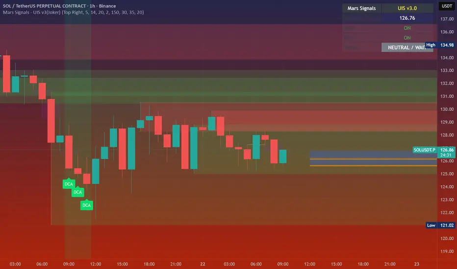
Mars Signals - Ultimate Institutional Suite v3.0(Joker)Comprehensive Trading Manual
Mars Signals – Ultimate Institutional Suite v3.0 (Joker)
## Chapter 1 – Philosophy & System Architecture
This script is not a simple “buy/sell” indicator.
Mars Signals – UIS v3.0 (Joker) is designed as an institutional-style analytical assistant that layers several methodologies into a single, coherent framework.
The system is built on four core pillars:
1. Smart Money Concepts (SMC)
- Detection of Order Blocks (professional demand/supply zones).
- Detection of Fair Value Gaps (FVGs) (price imbalances).
2. Smart DCA Strategy
- Combination of RSI and Bollinger Bands
- Identifies statistically discounted zones for scaling into spot positions or exiting shorts.
3. Volume Profile (Visible Range Simulation)
- Distribution of volume by price, not by time.
- Identification of POC (Point of Control) and high-/low-volume areas.
4. Wyckoff Helper – Spring
- Detection of bear traps, liquidity grabs, and sharp bullish reversals.
All four pillars feed into a Confluence Engine (Scoring System).
The final output is presented in the Dashboard, with a clear, human-readable signal:
- STRONG LONG 🚀
- WEAK LONG ↗
- NEUTRAL / WAIT
- WEAK SHORT ↘
- STRONG SHORT 🩸
This allows the trader to see *how many* and *which* layers of the system support a bullish or bearish bias at any given time.
## Chapter 2 – Settings Overview
### 2.1 General & Dashboard Group
- Show Dashboard Panel (`show_dash`)
Turns the dashboard table in the corner of the chart ON/OFF.
- Show Signal Recommendation (`show_rec`)
- If enabled, the textual signal (STRONG LONG, WEAK SHORT, etc.) is displayed.
- If disabled, you only see feature status (ON/OFF) and the current price.
- Dashboard Position (`dash_pos`)
Determines where the dashboard appears on the chart:
- `Top Right`
- `Bottom Right`
- `Top Left`
### 2.2 Smart Money (SMC) Group
- Enable SMC Strategy (`show_smc`)
Globally enables or disables the Order Block and FVG logic.
- Order Block Pivot Lookback (`ob_period`)
Main parameter for detecting key pivot highs/lows (swing points).
- Default value: 5
- Concept:
A bar is considered a pivot low if its low is lower than the lows of the previous 5 and the next 5 bars.
Similarly, a pivot high has a high higher than the previous 5 and the next 5 bars.
These pivots are used as anchors for Order Blocks.
- Increasing `ob_period`:
- Fewer levels.
- But levels tend to be more significant and reliable.
- In highly volatile markets (major news, war events, FOMC, etc.),
using values 7–10 is recommended to filter out weak levels.
- Show Fair Value Gaps (`show_fvg`)
Enables/disables the drawing of FVG zones (imbalances).
- Bullish OB Color (`c_ob_bull`)
- Color of Bullish Order Blocks (Demand Zones).
- Default: semi-transparent green (transparency ≈ 80).
- Bearish OB Color (`c_ob_bear`)
- Color of Bearish Order Blocks (Supply Zones).
- Default: semi-transparent red.
- Bullish FVG Color (`c_fvg_bull`)
- Color of Bullish FVG (upward imbalance), typically yellow.
- Bearish FVG Color (`c_fvg_bear`)
- Color of Bearish FVG (downward imbalance), typically purple.
### 2.3 Smart DCA Strategy Group
- Enable DCA Zones (`show_dca`)
Enables the Smart DCA logic and visual labels.
- RSI Length (`rsi_len`)
Lookback period for RSI (default: 14).
- Shorter → more sensitive, more noise.
- Longer → fewer signals, higher reliability.
- Bollinger Bands Length (`bb_len`)
Moving average period for Bollinger Bands (default: 20).
- BB Multiplier (`bb_mult`)
Standard deviation multiplier for Bollinger Bands (default: 2.0).
- For extremely volatile markets, values like 2.5–3.0 can be used so that only extreme deviations trigger a DCA signal.
### 2.4 Volume Profile (Visible Range Sim) Group
- Show Volume Profile (`show_vp`)
Enables the simulated Volume Profile bars on the right side of the chart.
- Volume Lookback Bars (`vp_lookback`)
Number of bars used to compute the Volume Profile (default: 150).
- Higher values → broader historical context, heavier computation.
- Row Count (`vp_rows`)
Number of vertical price segments (rows) to divide the total price range into (default: 30).
- Width (%) (`vp_width`)
Relative width of each volume bar as a percentage.
In the code, bar widths are scaled relative to the row with the maximum volume.
> Technical note: Volume Profile calculations are executed only on the last bar (`barstate.islast`) to keep the script performant even on higher timeframes.
### 2.5 Wyckoff Helper Group
- Show Wyckoff Events (`show_wyc`)
Enables detection and plotting of Wyckoff Spring events.
- Volume MA Length (`vol_ma_len`)
Length of the moving average on volume.
A bar is considered to have Ultra Volume if its volume is more than 2× the volume MA.
## Chapter 3 – Smart Money Strategy (Order Blocks & FVG)
### 3.1 What Is an Order Block?
An Order Block (OB) represents the footprint of large institutional orders:
- Bullish Order Block (Demand Zone)
The last selling region (bearish candle/cluster) before a strong upward move.
- Bearish Order Block (Supply Zone)
The last buying region (bullish candle/cluster) before a strong downward move.
Institutions and large players place heavy orders in these regions. Typical price behavior:
- Price moves away from the zone.
- Later returns to the same zone to fill unfilled orders.
- Then continues the larger trend.
In the script:
- If `pl` (pivot low) forms → a Bullish OB is created.
- If `ph` (pivot high) forms → a Bearish OB is created.
The box is drawn:
- From `bar_index ` to `bar_index`.
- Between `low ` and `high `.
- `extend=extend.right` extends the OB into the future, so it acts as a dynamic support/resistance zone.
- Only the last 4 OB boxes are kept to avoid clutter.
### 3.2 Order Block Color Guide
- Semi-transparent Green (`c_ob_bull`)
- Represents a Bullish Order Block (Demand Zone).
- Interpretation: a price region with a high probability of bullish reaction.
- Semi-transparent Red (`c_ob_bear`)
- Represents a Bearish Order Block (Supply Zone).
- Interpretation: a price region with a high probability of bearish reaction.
Overlap (Multiple OBs in the Same Area)
When two or more Order Blocks overlap:
- The shared area appears visually denser/stronger.
- This suggests higher order density.
- Such zones can be treated as high-priority levels for entries, exits, and stop-loss placement.
### 3.3 Demand/Supply Logic in the Scoring Engine
is_in_demand = low <= ta.lowest(low, 20)
is_in_supply = high >= ta.highest(high, 20)
- If current price is near the lowest lows of the last 20 bars, it is considered in a Demand Zone → positive impact on score.
- If current price is near the highest highs of the last 20 bars, it is considered in a Supply Zone → negative impact on score.
This logic complements Order Blocks and helps the Dashboard distinguish whether:
- Market is currently in a statistically cheap (long-friendly) area, or
- In a statistically expensive (short-friendly) area.
### 3.4 Fair Value Gaps (FVG)
#### Concept
When the market moves aggressively:
- Some price levels are skipped and never traded.
- A gap between wicks/shadows of consecutive candles appears.
- These regions are called Fair Value Gaps (FVGs) or Imbalances.
The market generally “dislikes” imbalance and often:
- Returns to these zones in the future.
- Fills the gap (rebalance).
- Then resumes its dominant direction.
#### Implementation in the Code
Bullish FVG (Yellow)
fvg_bull_cond = show_smc and show_fvg and low > high and close > high
if fvg_bull_cond
box.new(bar_index , high , bar_index, low, ...)
Core condition:
`low > high ` → the current low is above the high of two bars ago; the space between them is an untraded gap.
Bearish FVG (Purple)
fvg_bear_cond = show_smc and show_fvg and high < low and close < low
if fvg_bear_cond
box.new(bar_index , low , bar_index, high, ...)
Core condition:
`high < low ` → the current high is below the low of two bars ago; again a price gap exists.
#### FVG Color Guide
- Transparent Yellow (`c_fvg_bull`) – Bullish FVG
Often acts like a magnet for price:
- Price tends to retrace into this zone,
- Fill the imbalance,
- And then continue higher.
- Transparent Purple (`c_fvg_bear`) – Bearish FVG
Price tends to:
- Retrace upward into the purple area,
- Fill the imbalance,
- And then resume downward movement.
#### Trading with FVGs
- FVGs are *not* standalone entry signals.
They are best used as:
- Targets (take-profit zones), or
- Reaction areas where you expect a pause or reversal.
Examples:
- If you are long, a bearish FVG above is often an excellent take-profit zone.
- If you are short, a bullish FVG below is often a good cover/exit zone.
### 3.5 Core SMC Trading Templates
#### Reversal Long
1. Price trades down into a green Order Block (Demand Zone).
2. A bullish confirmation candle (Close > Open) forms inside or just above the OB.
3. If this zone is close to or aligned with a bullish FVG (yellow), the signal is reinforced.
4. Entry:
- At the close of the confirmation candle, or
- Using a limit order near the upper boundary of the OB.
5. Stop-loss:
- Slightly below the OB.
- If the OB is broken decisively and price consolidates below it, the zone loses validity.
6. Targets:
- The next FVG,
- Or the next red Order Block (Supply Zone) above.
#### Reversal Short
The mirror scenario:
- Price rallies into a red Order Block (Supply).
- A bearish confirmation candle forms (Close < Open).
- FVG/premium structure above can act as a confluence.
- Stop-loss goes above the OB.
- Targets: lower FVGs or subsequent green OBs below.
## Chapter 4 – Smart DCA Strategy (RSI + Bollinger Bands)
### 4.1 Smart DCA Concept
- Classic DCA = buying at fixed time intervals regardless of price.
- Smart DCA = scaling in only when:
- Price is statistically cheaper than usual, and
- The market is in a clear oversold condition.
Code logic:
rsi_val = ta.rsi(close, rsi_len)
= ta.bb(close, bb_len, bb_mult)
dca_buy = show_dca and rsi_val < 30 and close < bb_lower
dca_sell = show_dca and rsi_val > 70 and close > bb_upper
Conditions:
- DCA Buy – Smart Scale-In Zone
- RSI < 30 → oversold.
- Close < lower Bollinger Band → price has broken below its typical volatility envelope.
- DCA Sell – Overbought/Distribution Zone
- RSI > 70 → overbought.
- Close > upper Bollinger Band → price is extended far above the mean.
### 4.2 Visual Representation on the Chart
- Green “DCA” Label Below Candle
- Shape: `labelup`.
- Color: lime background, white text.
- Meaning: statistically attractive level for laddered spot entries or short exits.
- Red “SELL” Label Above Candle
- Warning that the market is in an extended, overbought condition.
- Suitable for profit-taking on longs or considering short entries (with proper confluence and risk management).
- Light Green Background (`bgcolor`)
- When `dca_buy` is true, the candle background turns very light green (high transparency).
- This helps visually identify DCA Zones across the chart at a glance.
### 4.3 Practical Use in Trading
#### Spot Trading
Used to build a better average entry price:
- Every time a DCA label appears, allocate a fixed portion of capital (e.g., 2–5%).
- Combining DCA signals with:
- Green OBs (Demand Zones), and/or
- The Volume Profile POC
makes the zone structurally more important.
#### Futures Trading
- Longs
- Use DCA Buy signals as low-risk zones for opening or adding to longs when:
- Price is inside a green OB, or
- The Dashboard already leans LONG.
- Shorts
- Use DCA Sell signals as:
- Exit zones for longs, or
- Areas to initiate shorts with stops above structural highs.
## Chapter 5 – Volume Profile (Visible Range Simulation)
### 5.1 Concept
Traditional volume (histogram under the chart) shows volume over time.
Volume Profile shows volume by price level:
- At which prices has the highest trading activity occurred?
- Where did buyers and sellers agree the most (High Volume Nodes – HVNs)?
- Where did price move quickly due to low participation (Low Volume Nodes – LVNs)?
### 5.2 Implementation in the Script
Executed only when `show_vp` is enabled and on the last bar:
1. The last `vp_lookback` bars (default 150) are processed.
2. The minimum low and maximum high over this window define the price range.
3. This price range is divided into `vp_rows` segments (e.g., 30 rows).
4. For each row:
- All bars are scanned.
- If the mid-price `(high + low ) / 2` falls inside a row, that bar’s volume is added to the row total.
5. The row with the greatest volume is stored as `max_vol_idx` (the POC row).
6. For each row, a volume box is drawn on the right side of the chart.
### 5.3 Color Scheme
- Semi-transparent Orange
- The row with the maximum volume – the Point of Control (POC).
- Represents the strongest support/resistance level from a volume perspective.
- Semi-transparent Blue
- Other volume rows.
- The taller the bar → the higher the volume → the stronger the interest at that price band.
### 5.4 Trading Applications
- If price is above POC and retraces back into it:
→ POC often acts as support, suitable for long setups.
- If price is below POC and rallies into it:
→ POC often acts as resistance, suitable for short setups or profit-taking.
HVNs (Tall Blue Bars)
- Represent areas of equilibrium where the market has spent time and traded heavily.
- Price tends to consolidate here before choosing a direction.
LVNs (Short or Nearly Empty Bars)
- Represent low participation zones.
- Price often moves quickly through these areas – useful for targeting fast moves.
## Chapter 6 – Wyckoff Helper – Spring
### 6.1 Spring Concept
In the Wyckoff framework:
- A Spring is a false break of support.
- The market briefly trades below a well-defined support level, triggers stop losses,
then sharply reverses upward as institutional buyers absorb liquidity.
This movement:
- Clears out weak hands (retail sellers).
- Provides large players with liquidity to enter long positions.
- Often initiates a new uptrend.
### 6.2 Code Logic
Conditions for a Spring:
1. The current low is lower than the lowest low of the previous 50 bars
→ apparent break of a long-standing support.
2. The bar closes bullish (Close > Open)
→ the breakdown was rejected.
3. Volume is significantly elevated:
→ `volume > 2 × volume_MA` (Ultra Volume).
When all conditions are met and `show_wyc` is enabled:
- A pink diamond is plotted below the bar,
- With the label “Spring” – one of the strongest long signals in this system.
### 6.3 Trading Use
- After a valid Spring, markets frequently enter a meaningful bullish phase.
- The highest quality setups occur when:
- The Spring forms inside a green Order Block, and
- Near or on the Volume Profile POC.
Entries:
- At the close of the Spring bar, or
- On the first pullback into the mid-range of the Spring candle.
Stop-loss:
- Slightly below the Spring’s lowest point (wick low plus a small buffer).
## Chapter 7 – Confluence Engine & Dashboard
### 7.1 Scoring Logic
For each bar, the script:
1. Resets `score` to 0.
2. Adjusts the score based on different signals.
SMC Contribution
if show_smc
if is_in_demand
score += 1
if is_in_supply
score -= 1
- Being in Demand → `+1`
- Being in Supply → `-1`
DCA Contribution
if show_dca
if dca_buy
score += 2
if dca_sell
score -= 2
- DCA Buy → `+2` (strong, statistically driven long signal)
- DCA Sell → `-2`
Wyckoff Spring Contribution
if show_wyc
if wyc_spring
score += 2
- Spring → `+2` (entry of strong money)
### 7.2 Mapping Score to Dashboard Signal
- score ≥ 2 → STRONG LONG 🚀
Multiple bullish conditions aligned.
- score = 1 → WEAK LONG ↗
Some bullish bias, but only one layer clearly positive.
- score = 0 → NEUTRAL / WAIT
Rough balance between buying and selling forces; staying flat is usually preferable.
- score = -1 → WEAK SHORT ↘
Mild bearish bias, suited for cautious or short-term plays.
- score ≤ -2 → STRONG SHORT 🩸
Convergence of several bearish signals.
### 7.3 Dashboard Structure
The dashboard is a two-column table:
- Row 0
- Column 0: `"Mars Signals"` – black background, white text.
- Column 1: `"UIS v3.0"` – black background, yellow text.
- Row 1
- Column 0: `"Price:"` (light grey background).
- Column 1: current closing price (`close`) with a semi-transparent blue background.
- Row 2
- Column 0: `"SMC:"`
- Column 1:
- `"ON"` (green) if `show_smc = true`
- `"OFF"` (grey) otherwise.
- Row 3
- Column 0: `"DCA:"`
- Column 1:
- `"ON"` (green) if `show_dca = true`
- `"OFF"` (grey) otherwise.
- Row 4
- Column 0: `"Signal:"`
- Column 1: signal text (`status_txt`) with background color `status_col`
(green, red, teal, maroon, etc.)
- If `show_rec = false`, these cells are cleared.
## Chapter 8 – Visual Legend (Colors, Shapes & Actions)
For quick reading inside TradingView, the visual elements are described line by line instead of a table.
Chart Element: Green Box
Color / Shape: Transparent green rectangle
Core Meaning: Bullish Order Block (Demand Zone)
Suggested Trader Response: Look for longs, Smart DCA adds, closing or reducing shorts.
Chart Element: Red Box
Color / Shape: Transparent red rectangle
Core Meaning: Bearish Order Block (Supply Zone)
Suggested Trader Response: Look for shorts, or take profit on existing longs.
Chart Element: Yellow Area
Color / Shape: Transparent yellow zone
Core Meaning: Bullish FVG / upside imbalance
Suggested Trader Response: Short take-profit zone or expected rebalance area.
Chart Element: Purple Area
Color / Shape: Transparent purple zone
Core Meaning: Bearish FVG / downside imbalance
Suggested Trader Response: Long take-profit zone or temporary supply region.
Chart Element: Green "DCA" Label
Color / Shape: Green label with white text, plotted below the candle
Core Meaning: Smart ladder-in buy zone, DCA buy opportunity
Suggested Trader Response: Spot DCA entry, partial short exit.
Chart Element: Red "SELL" Label
Color / Shape: Red label with white text, plotted above the candle
Core Meaning: Overbought / distribution zone
Suggested Trader Response: Take profit on longs, consider initiating shorts.
Chart Element: Light Green Background (bgcolor)
Color / Shape: Very transparent light-green background behind bars
Core Meaning: Active DCA Buy zone
Suggested Trader Response: Treat as a discount zone on the chart.
Chart Element: Orange Bar on Right
Color / Shape: Transparent orange horizontal bar in the volume profile
Core Meaning: POC – price with highest traded volume
Suggested Trader Response: Strong support or resistance; key reference level.
Chart Element: Blue Bars on Right
Color / Shape: Transparent blue horizontal bars in the volume profile
Core Meaning: Other volume levels, showing high-volume and low-volume nodes
Suggested Trader Response: Use to identify balance zones (HVN) and fast-move corridors (LVN).
Chart Element: Pink "Spring" Diamond
Color / Shape: Pink diamond with white text below the candle
Core Meaning: Wyckoff Spring – liquidity grab and potential major bullish reversal
Suggested Trader Response: One of the strongest long signals in the suite; look for high-quality long setups with tight risk.
Chart Element: STRONG LONG in Dashboard
Color / Shape: Green background, white text in the Signal row
Core Meaning: Multiple bullish layers in confluence
Suggested Trader Response: Consider initiating or increasing longs with strict risk management.
Chart Element: STRONG SHORT in Dashboard
Color / Shape: Red background, white text in the Signal row
Core Meaning: Multiple bearish layers in confluence
Suggested Trader Response: Consider initiating or increasing shorts with a logical, well-placed stop.
## Chapter 9 – Timeframe-Based Trading Playbook
### 9.1 Timeframe Selection
- Scalping
- Timeframes: 1M, 5M, 15M
- Objective: fast intraday moves (minutes to a few hours).
- Recommendation: focus on SMC + Wyckoff.
Smart DCA on very low timeframes may introduce excessive noise.
- Day Trading
- Timeframes: 15M, 1H, 4H
- Provides a good balance between signal quality and frequency.
- Recommendation: use the full stack – SMC + DCA + Volume Profile + Wyckoff + Dashboard.
- Swing Trading & Position Investing
- Timeframes: Daily, Weekly
- Emphasis on Smart DCA + Volume Profile.
- SMC and Wyckoff are used mainly to fine-tune swing entries within larger trends.
### 9.2 Scenario A – Scalping Long
Example: 5-Minute Chart
1. Price is declining into a green OB (Bullish Demand).
2. A candle with a long lower wick and bullish close (Pin Bar / Rejection) forms inside the OB.
3. A Spring diamond appears below the same candle → very strong confluence.
4. The Dashboard shows at least WEAK LONG ↗, ideally STRONG LONG 🚀.
5. Entry:
- On the close of the confirmation candle, or
- On the first pullback into the mid-range of that candle.
6. Stop-loss:
- Slightly below the OB.
7. Targets:
- Nearby bearish FVG above, and/or
- The next red OB.
### 9.3 Scenario B – Day-Trading Short
Recommended Timeframes: 1H or 4H
1. The market completes a strong impulsive move upward.
2. Price enters a red Order Block (Supply).
3. In the same zone, a purple FVG appears or remains unfilled.
4. On a lower timeframe (e.g., 15M), RSI enters overbought territory and a DCA Sell signal appears.
5. The main timeframe Dashboard (1H) shows WEAK SHORT ↘ or STRONG SHORT 🩸.
Trade Plan
- Open a short near the upper boundary of the red OB.
- Place the stop above the OB or above the last swing high.
- Targets:
- A yellow FVG lower on the chart, and/or
- The next green OB (Demand) below.
### 9.4 Scenario C – Swing / Investment with Smart DCA
Timeframes: Daily / Weekly
1. On the daily or weekly chart, each time a green “DCA” label appears:
- Allocate a fixed fraction of your capital (e.g., 3–5%) to that asset.
2. Check whether this DCA zone aligns with the orange POC of the Volume Profile:
- If yes → the quality of the entry zone is significantly higher.
3. If the DCA signal sits inside a daily green OB, the probability of a medium-term bottom increases.
4. Always build the position laddered, never all-in at a single price.
Exits for investors:
- Near weekly red OBs or large purple FVG zones.
- Ideally via partial profit-taking rather than closing 100% at once.
### 9.5 Case Study 1 – BTCUSDT (15-Minute)
- Context: Price has sold off down towards 65,000 USD.
- A green OB had previously formed at that level.
- Near the lower boundary of this OB, a partially filled yellow FVG is present.
- As price returns to this region, a Spring appears.
- The Dashboard shifts from NEUTRAL / WAIT to WEAK LONG ↗.
Plan
- Enter a long near the OB low.
- Place stop below the Spring low.
- First target: a purple FVG around 66,200.
- Second (optional) target: the first red OB above that level.
### 9.6 Case Study 2 – Meme Coin (PEPE – 4H)
- After a strong pump, price enters a corrective phase.
- On the 4H chart, RSI drops below 30; price breaks below the lower Bollinger Band → a DCA label prints.
- The Volume Profile shows the POC at approximately the same level.
- The Dashboard displays STRONG LONG 🚀.
Plan
- Execute laddered buys in the combined DCA + POC zone.
- Place a protective stop below the last significant swing low.
- Target: an expected 20–30% upside move towards the next red OB or purple FVG.
## Chapter 10 – Risk Management, Psychology & Advanced Tuning
### 10.1 Risk Management
No signal, regardless of its strength, replaces risk control.
Recommendations:
- In futures, do not expose more than 1–3% of account equity to risk per trade.
- Adjust leverage to the volatility of the instrument (lower leverage for highly volatile altcoins).
- Place stop-losses in zones where the idea is clearly invalidated:
- Below/above the relevant Order Block or Spring, not randomly in the middle of the structure.
### 10.2 Market-Specific Parameter Tuning
- Calmer Markets (e.g., major FX pairs)
- `ob_period`: 3–5.
- `bb_mult`: 2.0 is usually sufficient.
- Highly Volatile Markets (Crypto, news-driven assets)
- `ob_period`: 7–10 to highlight only the most robust OBs.
- `bb_mult`: 2.5–3.0 so that only extreme deviations trigger DCA.
- `vol_ma_len`: increase (e.g., to ~30) so that Spring triggers only on truly exceptional
volume spikes.
### 10.3 Trading Psychology
- STRONG LONG 🚀 does not mean “risk-free”.
It means the probability of a successful long, given the model’s logic, is higher than average.
- Treat Mars Signals as a confirmation and context system, not a full replacement for your own decision-making.
- Example of disciplined thinking:
- The Dashboard prints STRONG LONG,
- But price is simultaneously testing a multi-month macro resistance or a major negative news event is imminent,
- In such cases, trade smaller, widen stops appropriately, or skip the trade.
## Chapter 11 – Technical Notes & FAQ
### 11.1 Does the Script Repaint?
- Order Blocks and Springs are based on completed pivot structures and confirmed candles.
- Until a pivot is confirmed, an OB does not exist; after confirmation, behavior is stable under classic SMC assumptions.
- The script is designed to be structurally consistent rather than repainting signals arbitrarily.
### 11.2 Computational Load of Volume Profile
- On the last bar, the script processes up to `vp_lookback` bars × `vp_rows` rows.
- On very low timeframes with heavy zooming, this can become demanding.
- If you experience performance issues:
- Reduce `vp_lookback` or `vp_rows`, or
- Temporarily disable Volume Profile (`show_vp = false`).
### 11.3 Multi-Timeframe Behavior
- This version of the script is not internally multi-timeframe.
All logic (OB, DCA, Spring, Volume Profile) is computed on the active timeframe only.
- Practical workflow:
- Analyze overall structure and key zones on higher timeframes (4H / Daily).
- Use lower timeframes (15M / 1H) with the same tool for timing entries and exits.
## Conclusion
Mars Signals – Ultimate Institutional Suite v3.0 (Joker) is a multi-layer trading framework that unifies:
- Price structure (Order Blocks & FVG),
- Statistical behavior (Smart DCA via RSI + Bollinger),
- Volume distribution by price (Volume Profile with POC, HVN, LVN),
- Liquidity events (Wyckoff Spring),
into a single, coherent system driven by a transparent Confluence Scoring Engine.
The final output is presented in clear, actionable language:
> STRONG LONG / WEAK LONG / NEUTRAL / WEAK SHORT / STRONG SHORT
The system is designed to support professional decision-making, not to replace it.
Used together with strict risk management and disciplined execution,
Mars Signals – UIS v3.0 (Joker) can serve as a central reference manual and operational guide
for your trading workflow, from scalping to swing and investment positioning.
Average Price Calculator / VisualizerDCA Average Price Calculator - Visualize Your Breakeven & TP!
Ever wished you could visualize your trades and instantly see your average entry price right here on TradingView? Especially if you're a DCA (Dollar-Cost Averaging) trader like me, tracking multiple entries can be a hassle. You're constantly switching to a spreadsheet or calculator to figure out your breakeven and take-profit levels. Well I've developed this DCA Average Price Calculator to solve exactly that problem, bringing all your position planning directly onto your chart.
What It Does
This indicator is a interactive tool designed to calculate the weighted average price of up to 10 separate trade entries. It then plots your crucial breakeven (average price) and a customizable take-profit target directly on your chart, giving you a clear visual of your position.
Key Features
Up to 10 Order Entries: Plan complex DCA strategies with support for up to ten individual buys.
Flexible Size Input: Enter your position size in either USD Amount or Number of Shares/Contracts. The script is smart enough to know which one you're using.
Instant Average Price Calculation: Your weighted average price (your breakeven point) is calculated and plotted in real-time as a clean yellow line.
Customizable Take-Profit Target: Set your desired profit percentage and see your take-profit level instantly plotted as a green line.
Detailed On-Chart Labels: Each order you plot is marked with a detailed label showing the entry price, the number of shares purchased, and the total USD value of that entry.
Clean & Uncluttered UI: The main Average and TP labels are intelligently shifted to the right, ensuring they don't overlap with your entry markers, keeping your chart readable.
How to Use It - Simple Steps
Add the indicator to your chart.
Open the script's 'Settings' menu.
In the 'Take Profit' section, set your desired profit percentage (e.g., 1 for 1%).
Under the 'Orders' section, begin filling in your entries. For each 'Order #', enter the Price.
Next, enter the size. You can either fill in the 'Size (USD)' box OR the '/ Shares' box. Leave the one you're not using at 0.
As you add orders, the 'Avg' (yellow) and 'TP' (green) lines, along with the blue order labels, will automatically appear and adjust on your chart!
Who Is This For?
DCA Traders: This is the ultimate tool for you!
Position Traders: Keep track of scaling into a larger position over time.
Manual Backtesters: Quickly simulate and visualize how a series of buys would have played out.
Any Trader who wants a quick and easy way to calculate their average entry without leaving TradingView.
I built this tool to improve my own trading workflow, and I hope it helps you as much as it has helped me. If you find it useful, please consider giving it a 'Like' and feel free to leave any feedback or suggestions in the comments!
Happy trading

Basic DCA Strategy by Wongsakon KhaisaengThe Core Principle and Philosophy Behind the Basic DCA Strategy
1. Introduction
The Basic DCA Strategy (Dollar-Cost Averaging) represents one of the most fundamental and enduring investment methodologies in the realm of systematic accumulation. The philosophy underpinning DCA is rooted not in speculation or prediction, but in disciplined participation. It assumes that the consistent act of investing a fixed amount of capital over time—regardless of short-term price volatility—can yield superior long-term outcomes through the natural smoothing effect of cost averaging.
This strategy, expressed through the Pine Script code above, formalizes the DCA concept into a fully systematic trading framework, enabling quantitative backtesting and objective evaluation of long-term accumulation efficiency.
2. Mechanism of Operation
At its technical core, the strategy executes a fixed-value buy order at every predefined interval within a specific accumulation period.
Each DCA event invests a constant “Investment Amount (USD)” irrespective of price fluctuations. When prices decline, this constant investment buys a larger quantity of the asset; when prices rise, it purchases fewer units. Over time, this behavior lowers the average cost basis of the accumulated position, effectively neutralizing short-term timing risks.
Mathematically, this is represented as:
Units Purchased = Investment Amount / Closing Price
Cost Basis = Total Invested USD / Total Units Acquired
Portfolio Value = Total Units Acquired × Current Price
The algorithm tracks cumulative investment, acquired units, and commissions dynamically, continuously recalculating key portfolio metrics such as total profit/loss (PnL), CAGR (Compound Annual Growth Rate), and maximum drawdown (peak-to-trough equity decline).
Furthermore, the script juxtaposes DCA results with a Buy & Hold benchmark, where the entire initial capital is invested at once. This comparison highlights the behavioral resilience and volatility resistance of the DCA method relative to market-timing strategies.
3. The Essence of DCA Philosophy
At its philosophical core, DCA is not a trading system, but a behavioral framework for rational capital deployment under uncertainty. It embodies the principle that time in the market often outweighs timing the market.
The DCA approach rejects the illusion of precision forecasting and embraces probabilistic humility—the recognition that even the most skilled investors cannot consistently predict short-term market fluctuations. Instead, it focuses on controlling what is controllable: the frequency, consistency, and size of investment actions.
This mindset reflects a broader principle of risk dispersion through temporal diversification. Rather than concentrating entry risk into a single price point (as in lump-sum investing), DCA spreads exposure across multiple time intervals, thereby converting volatility into opportunity.
In essence, volatility—often perceived as risk—is reframed as a mechanism for mean reversion advantage. The strategy thrives precisely because markets oscillate; each fluctuation provides a chance to accumulate at varied price levels, improving the weighted-average entry over time.
4. Long-Term Rationality Over Short-Term Emotion
DCA’s endurance stems from its ability to neutralize emotional biases inherent in human decision-making. Investors tend to overreact to market euphoria or panic—buying high out of greed and selling low out of fear. By automating purchases through predefined intervals, the DCA model enforces mechanical discipline, detaching decision-making from sentiment.
This transforms investing from an emotional endeavor into a systematic, algorithmic routine governed by rules rather than reactions. In doing so, DCA serves not only as a financial model but also as a psychological safeguard—aligning investor behavior with long-term compounding logic rather than short-term speculation.
5. Comparative Insight: DCA vs. Buy & Hold
While both DCA and Buy & Hold share a long-term investment horizon, they diverge in their treatment of entry timing. The Buy & Hold model assumes full deployment of capital at the beginning, maximizing exposure to growth but also to volatility. Conversely, DCA smooths the entry curve, trading off short-term returns for long-term stability and improved average entry price.
In environments characterized by volatility and cyclical corrections, DCA tends to outperform in terms of risk-adjusted returns, lower drawdowns, and improved investor adherence—since it reduces the psychological pain of entering at local peaks.
6. Conclusion
The Basic DCA Strategy exemplifies the synthesis of mathematical rigor and behavioral discipline. Its algorithmic construction in Pine Script transforms a classical investment philosophy into a quantifiable, testable, and transparent framework.
By automating fixed-amount purchases across time, the system operationalizes the central axiom of DCA: consistency over conviction. It is not concerned with predicting future prices but with ensuring persistent participation—trusting that the market’s upward bias and the power of compounding will reward patience more than precision.
Ultimately, DCA embodies the timeless principle that successful investing is less about forecasting markets, and more about designing behavior that can endure them.

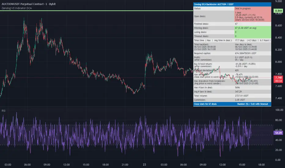
Zendog V3 Indicator DCAThis strategy is same as Zendog v3 but edited to be backtest compatible for SO additions through indicator
for Longs
Safety order type = External indicator
External indicator = RSI 30/70 : Long Trigger
Safety Order Value = 1
for Shorts
Safety order type = External indicator
External indicator = RSI 30/70 : Short Trigger
Safety Order Value = 2
DCA Percent SignalOverview
The DCA Percent Signal Indicator generates buy and sell signals based on percentage drops from all-time highs and percentage gains from lowest lows since ATH. This indicator is designed for pyramiding strategies where each signal represents a configurable percentage of equity allocation.
Definitions
DCA (Dollar-Cost Averaging): An investment strategy where you invest a fixed amount at regular intervals, regardless of price fluctuations. This indicator generates signals for a DCA-style pyramiding approach.
Gann Bar Types: Classification system for price bars based on their relationship to the previous bar:
Up Bar: High > previous high AND low ≥ previous low
Down Bar: High ≤ previous high AND low < previous low
Inside Bar: High ≤ previous high AND low ≥ previous low
Outside Bar: High > previous high AND low < previous low
ATH (All-Time High): The highest price level reached during the entire chart period
ATL (All-Time Low): The lowest price level reached since the most recent ATH
Pyramiding: A trading strategy that adds to positions on favorable price movements
Look-Ahead Bias: Using future information that wouldn't be available in real-time trading
Default Properties
Signal Thresholds:
Buy Threshold: 10% (triggers every 10% drop from ATH)
Sell Threshold: 30% (triggers every 30% gain from lowest low since ATH)
Price Sources:
ATH Tracking: High (ATH detection)
ATL Tracking: Low (low detection)
Buy Signal Source: Low (buy signals)
Sell Signal Source: High (sell signals)
Filter Options:
Apply Gann Filter: False (disabled by default)
Buy Sets ATL: False (disabled by default)
Display Options:
Show Buy/Sell Signals: True
Show Reference Lines: True
Show Info Table: False
Show Bar Type: False
How It Works
Buy Signals: Trigger every 10% drop from the all-time highest price reached
Sell Signals: Trigger every 30% increase from the lowest low since the most recent all-time high
Smart Tracking: Uses configurable price sources for signal generation
Key Features
Configurable Thresholds: Adjustable buy/sell percentage thresholds (default: 10%/30%)
Separate Price Sources: Independent sources for ATH tracking, ATL tracking, and signal triggers
Configurable Signals: Uses low for buy signals and high for sell signals by default
Optional Gann Filter: Apply Gann bar analysis for additional signal filtering
Optional Buy Sets ATL: Option to set ATL reference point when buy signals occur
Visual Debug: Detailed labels showing signal parameters and values
Usage Instructions
Apply to Chart: Use on any timeframe (recommended: 1D or higher for better signal quality)
Risk Management: Adjust thresholds based on your risk tolerance and market volatility
Signal Analysis: Monitor debug labels for detailed signal information and validation
Signal Logic
Buy signals are blocked when ATH increases to prevent buying at peaks
Sell signals are blocked when ATL decreases to prevent selling at lows
This ensures signals only trigger on subsequent bars, not the same bar that establishes new reference points
Buy Signals:
Calculate drop percentage from ATH to buy signal source
Trigger when drop reaches threshold increments (10%, 20%, 30%, etc.)
Always blocked on ATH bars to prevent buying at peaks
Optional: Also blocked on up/outside bars when Gann filter enabled
Sell Signals:
Calculate gain percentage from lowest low to sell signal source
Trigger when gain reaches threshold increments (30%, 60%, 90%, etc.)
Always blocked when ATL decreases to prevent selling at lows
Optional: Also blocked on down bars when Gann filter enabled
Limitations
Designed for trending markets; may generate many signals in sideways/ranging markets
Requires sufficient price movement to be effective
Not suitable for scalping or very short timeframes
Implementation Notes
Signals use optimistic price sources (low for buys, high for sells), these can be configured to be more conservative
Gann filter provides additional signal filtering based on bar types
Debug information available in data window for real-time analysis
Detailed labels on each signal show ATH, lowest low, buy level, sell level, and drop/gain percentages

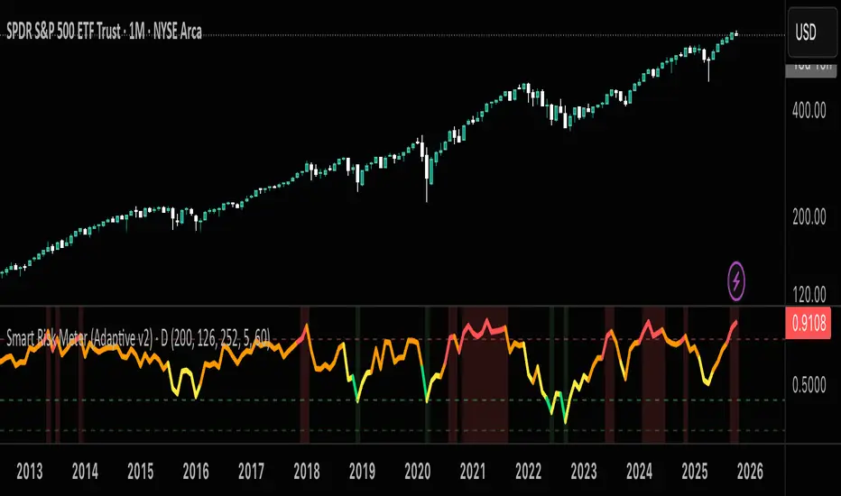
Smart Risk DCA Meter — Adaptive Market Risk EngineThe **Smart Risk DCA Meter** is an adaptive market-risk indicator that helps you invest smarter by scaling your DCA buys based on actual market conditions instead of emotion. It combines momentum, distance from trend, and drawdown factors into a single 0–1 risk score that automatically adjusts to each asset’s volatility — from stable indices like SPX to high-beta assets like BTC. Low readings (green zones) signal opportunity to buy heavier, while high readings (red zones) warn to slow down and protect capital.
DCA with the Money Supply Index DCA with the Money Supply Index (MSI) by zdmre
This strategy is based on the Money Supply Index (MSI) by zdmre and enhances it with two functional options for users: a DCA (Dollar-Cost Averaging) approach and a signal-based buy/sell mode. It’s designed to help traders and investors make data-driven, disciplined entry decisions based on monetary supply trends.
🧠 Concept Overview
The Money Supply Index (MSI) provides insight into how liquidity (money supply) influences market movements. This strategy builds upon that foundation by allowing users to either:
Accumulate positions over time using DCA, based on favorable MSI conditions.
Execute a single buy and sell trade, optimized for bull market conditions.
⚙️ Inputs Explained
General Parameters
Start Bar Index / Stop Bar Index
Defines the range of bars (historical data) for backtesting or strategy visualization.
Long DCA
Activates the DCA mode. If unchecked, the strategy operates in single-entry/single-exit signal mode.
Trading Signal
Enables signal-based entries and exits when the MSI reaches predefined thresholds.
DCA Parameters
Entry Value
The MSI value that triggers a DCA buy event. When the MSI crosses below this value, the strategy considers it a favorable moment to deploy the saved capital.
Saved Amount
The amount of money set aside regularly (e.g., monthly) for investment. This simulates the DCA effect by accumulating capital and deploying it when conditions are optimal.
Data Inputs
Money Supply
The data source for the Money Supply Index (default: ECONOMICS:USM2).
Relational Symbol
The market instrument to compare against the money supply (default: NASDAQ_DLY:NDX). This allows the strategy to measure liquidity impact on a specific market.
Chart Display Options
You can toggle these metrics on the chart for better visualization:
Entry Price (green) – The price level of executed buys.
Cash Balance (yellow) – Remaining uninvested capital.
Invested Capital (red) – Total amount currently invested.
Current Value (blue) – The current valuation of the investment.
Profit (purple) – The total realized and unrealized profit.
Trades on Chart / Signal Labels / Quantity – Enables trade markers, signal text, and position size visualization.
📈 How the Strategy Works
1️⃣ DCA Mode
In DCA mode, the strategy simulates periodic savings and only invests when the MSI indicates favorable liquidity conditions (based on the Entry Value).
This approach aims to achieve the best possible average entry price over time — a powerful strategy for long-term investors seeking stable accumulation with reduced emotional bias.
2️⃣ Signal-Based Mode
In signal mode (with DCA disabled), the strategy performs one buy and one sell trade based on MSI turning points.
It’s most effective during bull markets, where liquidity expansion supports upward momentum.
This mode helps identify high-probability entry and exit zones rather than averaging in continuously.
💡 Additional Notes
This strategy includes helpful metrics to monitor your personal investment performance — showing invested capital, cash reserves, and profit in real-time.
The goal is to combine macroeconomic insight (money supply) with disciplined execution and capital management.
⚠️ Disclaimer
This strategy is for educational and research purposes only. It does not constitute financial advice. Always conduct your own analysis before making investment decisions.

Cost Basis of DCA Strategy (Enhanced)“Cost Basis of DCA Strategy (Enhanced): An Analytical Tool for Smarter DCA Investing”
The indicator designed here serves as a comprehensive analytical tool for evaluating a Dollar-Cost Averaging (DCA) strategy. Instead of merely recording scattered buy transactions, it integrates all purchases into a clear framework that reveals the real cost basis, portfolio performance, and capital allocation. Its primary function is to transform the concept of DCA from a mechanical process into a measurable and strategic decision-making system.
At the foundation of its operation, the user provides essential inputs such as the initial capital, the price and size of each buy transaction, and an optional sell price for hypothetical exit scenarios. With these inputs, the indicator calculates how many units were acquired in total, how much money was spent, and what the average cost per unit—the cost basis—truly is. This cost basis acts as the anchor for evaluating whether the market price has moved in favor or against the investor’s average entry point.
Beyond this, the indicator goes further by calculating both realized and unrealized dimensions of performance. It presents the current market value of holdings based on live price data and contrasts it with the total cost to derive unrealized profit or loss in both absolute terms and percentages. If the user sets a sell price, the tool simulates a full liquidation scenario, displaying the expected profit or loss should all holdings be sold at that level. This dual perspective enables the user to examine their strategy both from a present-value standpoint and a forward-looking one.
In addition, the indicator keeps track of remaining capital—the portion of initial funds not yet deployed into purchases—thus bridging the gap between portfolio construction and financial planning. It also reports the number of buy transactions, reinforcing awareness of execution discipline in DCA.
For visualization, the system is not confined to numbers alone. It marks each buy price directly on the price chart with distinct horizontal lines, labeled for clarity. This allows the trader to see not just statistics in a table but also the spatial relationship between historical entry points and ongoing market dynamics.
In essence, this indicator reframes the practice of DCA into a structured analytical exercise. It empowers investors to understand the true average entry cost, evaluate ongoing performance, and simulate future outcomes under different price scenarios. By doing so, it elevates DCA from a passive habit into an active, data-driven investment methodology, allowing users to make more informed, confident, and strategically grounded decisions.
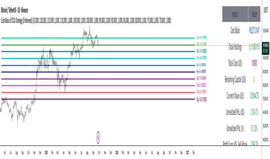
DCA Anchor (Weekly/Monthly/N Bars) [CHE] What is Dollar-Cost Averaging (DCA)?
DCA is a position-building method where you invest a fixed amount at fixed intervals (e.g., weekly or monthly) regardless of price. Over time, this:
reduces timing risk (you don’t need to guess tops/bottoms),
smooths entry price by buying more units when price is low and fewer when price is high,
keeps decisions simple and repeatable.
Trade-offs:
You’ll never catch the exact bottom.
In strong uptrends, lump-sum can outperform.
Fees matter if you buy very frequently.
Simple math:
Qty bought at time t = `amount / price_t` (net of fees if fees are not “on top”).
Total qty = sum of all buys.
Average price (cost basis) = `total invested / total qty`.
Equity = `total qty last price`.
P\&L = `equity − total invested` (and `%` = `P&L / total invested`).
DCA Anchor (Weekly/Monthly/N Bars)
Purpose: automate scheduled DCA buys on chart data, optionally add extra buys on drawdowns, track stats, and fire alerts.
Core features
Schedules:
1. Every N bars,
2. Weekly (first bar of a new week),
3. Monthly (first bar of a new month).
A Start time input gates when the logic begins.
Fees model:
Fee on top: you pay `amount + fee` in cash; quantity = `amount / close`.
Fee from amount: fee is deducted from the amount; quantity is smaller, cash outlay equals `amount`.
Optional drawdown buys:
Trigger when `close ≤ avgCost (1 − ddPct/100)`.
Controls: drawdown % threshold, multiplier (extra size vs. base amount), and cooldown in bars.
State & metrics: tracks total invested, total quantity, average price, equity, P\&L (abs/%).
Visuals:
Line plot of Average Price.
Buy labels at execution bars (plan and drawdown).
Compact table (positionable) with key stats (trades, invested, qty, avg price, equity, P\&L).
Alerts:
Plan Buy (Bar Close) and Drawdown Buy (Bar Close) — robust, non-repainting.
Optional Intrabar Preview alerts for early heads-up (can fire before bar close).
How to use it (quick start)
1. Add to chart → Inputs:
Buy frequency: pick Every N bars, Weekly, or Monthly.
Start time: date from which buys may begin.
Buy amount: fixed cash per planned buy.
Fees % and Fee on top? to match your broker/exchange model.
(Optional) Enable drawdown buy, set threshold %, multiplier, and cooldown.
Toggle Show buy labels and Show stats table.
2. Alerts (recommended):
Use “DCA Plan Buy (Bar Close)” and/or “DCA Drawdown Buy (Bar Close)” with Once per bar close.
If you need early signals, enable Intrabar pre-alerts and add the two Intrabar Preview alerts with Once per bar.
3. Interpretation:
The yellow line is your average price.
Green/orange markers show plan buys and drawdown buys.
The table summarizes total trades, invested capital, quantity, average price, current equity, and P\&L.
Practical notes
All executions occur at bar close by default to avoid intrabar repainting.
Weekly/monthly roll depends on the symbol’s exchange calendar.
Backtest realism: no slippage, no partial fills. Fees are modeled as configured.
If you buy very frequently, consider higher “N” or weekly/monthly to keep fees under control.
If you want, I can tailor the defaults (amount, fee model, drawdown rules) to your typical markets and timeframes.
Disclaimer
No indicator guarantees profits. DCA Anchor (Weekly/Monthly/N Bars) is a decision aid; always combine with solid risk management and your own judgment. Backtest, forward test, and size responsibly.
The content provided, including all code and materials, is strictly for educational and informational purposes only. It is not intended as, and should not be interpreted as, financial advice, a recommendation to buy or sell any financial instrument, or an offer of any financial product or service. All strategies, tools, and examples discussed are provided for illustrative purposes to demonstrate coding techniques and the functionality of Pine Script within a trading context.
Any results from strategies or tools provided are hypothetical, and past performance is not indicative of future results. Trading and investing involve high risk, including the potential loss of principal, and may not be suitable for all individuals. Before making any trading decisions, please consult with a qualified financial professional to understand the risks involved.
By using this script, you acknowledge and agree that any trading decisions are made solely at your discretion and risk.
Enhance your trading precision and confidence 🚀
Best regards
Chervolino

Mean Reversion Channel [QuantAlgo]🟢 Overview
The Mean Reversion Channel indicator is a range-bound trading system that combines dynamic price channels with momentum-weighted analysis to identify optimal mean reversion opportunities. It creates adaptive upper and lower reversion zones based on recent price action and volatility, while incorporating a momentum-biased equilibrium line that shifts based on volume-weighted price momentum. This creates a three-tier system where traders and investors can identify overbought and oversold conditions within established ranges, detect momentum exhaustion points, and anticipate channel breakouts or breakdowns. This indicator is particularly valuable for strategic dollar cost averaging (DCA) strategies, as it helps identify optimal accumulation zones during oversold conditions and provides tactical risk management levels for systematic investment approaches across different market conditions and asset classes.
🟢 How It Works
The indicator employs a four-stage calculation process that transforms raw price and volume data into actionable mean reversion signals. First, it establishes the base channel by calculating the highest high and lowest low over a user-defined lookback period, creating the foundational price range for mean reversion analysis. This channel adapts continuously as new price data becomes available, ensuring the system remains relevant to current market conditions.
In the second stage, the system calculates volume-weighted momentum by combining price momentum with volume activity. The momentum calculation takes the price change over a specified period and multiplies it by the volume ratio (current volume versus 20-period average volume, for instance) and a volume factor multiplier. This creates momentum readings that are more significant during high-volume periods and less influential during low-volume conditions.
The third stage creates the dynamic reversion zones using Average True Range (ATR) calculations. The upper reversion zone is positioned below the channel high by an ATR-based distance, while the lower reversion zone is positioned above the channel low. These zones contract when momentum is negative (upper zone) or positive (lower zone), creating asymmetric reversion bands that adapt to momentum conditions.
The final stage establishes the momentum-biased equilibrium line by calculating the midpoint between the reversion zones and adjusting it based on momentum bias. When momentum is positive, the equilibrium shifts upward; when negative, it shifts downward. This creates a dynamic reference level that helps identify when price action is moving against the prevailing momentum trend, signaling potential mean reversion opportunities.
🟢 How to Use
1. Mean Reversion Signal Identification
Lower Reversion Zone Signals: When price reaches or falls below the lower reversion zone with bearish momentum, the system generates potential long/buy entry signals indicating oversold conditions within the established range.
Upper Reversion Zone Signals: When price reaches or exceeds the upper reversion zone with bullish momentum, the system generates potential short/sell entry signals indicating overbought conditions.
2. Equilibrium Line Analysis and Momentum Exhaustion
Equilibrium Breaks: The dynamic equilibrium line serves as a momentum bias indicator within the channel. Price crossing above equilibrium suggests shifting to bullish bias, while breaks below indicate bearish bias development within the mean reversion framework.
Momentum Exhaustion Signals: The system identifies momentum exhaustion when price breaks through the equilibrium line opposite to the prevailing momentum direction. Bullish exhaustion occurs when price falls below equilibrium despite positive momentum, while bearish exhaustion happens when price rises above equilibrium during negative momentum periods.
3. Channel Expansion and Breakout Detection
Channel Boundary Breaks: When price breaks above the upper reversion zone or below the lower reversion zone, it signals potential channel expansion or false breakout conditions. These events often precede significant trend changes or range expansion phases.
Range Expansion Alerts: Breaks above the channel high or below the channel low indicate potential breakout from the mean reversion range, suggesting trend continuation or new directional movement beyond the established boundaries.
🟢 Pro Tips for Trading and Investing
→ Strategic DCA Optimization: Use the lower reversion zone as primary accumulation levels for dollar cost averaging strategies. When price reaches oversold conditions with bearish momentum exhaustion signals, it often represents optimal entry points for systematic investment programs, allowing investors to accumulate positions at statistically favorable price levels within the established range.
→ DCA Pause and Acceleration Signals : Monitor equilibrium line breaks to adjust DCA frequency and amounts. When price consistently trades below equilibrium with momentum exhaustion signals, consider accelerating DCA intervals or increasing investment amounts. Conversely, when price reaches upper reversion zones, consider pausing or reducing DCA activity until more favorable conditions return.
→ Momentum Divergence Detection: Watch for divergences between price action and momentum readings within the channel. When price makes new lows but momentum shows improvement, or price makes new highs with deteriorating momentum, these signal high-probability mean reversion setups ideal for contrarian investment approaches.
→ Alert-Based Systematic Investing/Trading: Utilize the comprehensive alert system for automated DCA triggers. Set up alerts for lower reversion zone touches combined with momentum exhaustion signals to create systematic entry points that remove emotional decision-making from long-term investment strategies, particularly effective for volatile assets where timing improvements can significantly impact overall returns.
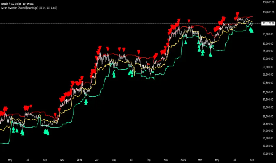
Crypto Perp Calc v1Advanced Perpetual Position Calculator for TradingView
Description
A comprehensive position sizing and risk management tool designed specifically for perpetual futures trading. This indicator eliminates the confusion of calculating leveraged positions by providing real-time position metrics directly on your chart.
Key Features:
Interactive Price Selection: Click directly on chart to set entry, stop loss, and take profit levels
Accurate Lot Size Calculation: Instantly calculates the exact position size needed for your margin and leverage
Multiple Entry Support: DCA into positions with up to 3 entry points with customizable allocation
Multiple Take Profit Levels: Scale out of positions with up to 3 TP targets
Comprehensive Risk Metrics: Shows dollar P&L, account risk percentage, and liquidation price
Visual Risk/Reward: Color-coded boxes and lines display your trade setup clearly
Real-time Info Table: All critical position data in one organized panel
Perfect for traders using perpetual futures who need precise position sizing with leverage.
---------
How to Use
Quick Start (3 Clicks)
1. Add the indicator to your chart
2. Click three times when prompted:
First click: Set your entry price
Second click: Set your stop loss
Third click: Set your take profit
3. Read the TOTAL LOTS value from the info table (highlighted in yellow)
4. Use this lot size in your exchange when placing the trade
Detailed Setup
Step 1: Configure Your Account
Enter your account balance (total USDT in account)
Set your margin amount (how much USDT to risk on this trade)
Choose your leverage (1x to 125x)
Select Long or Short position
Step 2: Set Price Levels
Main levels use interactive clicking (Entry, SL, TP)
For multiple entries or TPs, use the settings panel to manually input prices and percentages
Step 3: Read the Results
The info table shows:
TOTAL LOTS - The position size to enter on your exchange
Margin Used - Your actual capital at risk
Notional - Total position value (margin × leverage)
Max Risk - Dollar amount you'll lose at stop loss
Total Profit - Dollar amount you'll gain at take profit
R:R Ratio - Risk to reward ratio
Account Risk - Percentage of account at risk
Liquidation - Price where position gets liquidated
Step 4: Advanced Features (Optional)
Multiple Entries (DCA):
Enable "Use Multiple Entries"
Set up to 3 entry prices
Allocate percentage for each (must total 100%)
See individual lot sizes for each entry
Multiple Take Profits:
Enable "Use Multiple TPs"
Set up to 3 TP levels
Allocate percentage to close at each level (must total 100%)
View profit at each target
Visual Elements
Blue lines/labels: Entry points
Red lines/labels: Stop loss
Green lines/labels: Take profit targets
Colored boxes: Visual risk (red) and reward (green) zones
Info table: Can be positioned anywhere on screen
Alerts
Set price alerts for:
Entry zones reached
Stop loss approached
Take profit levels hit
Works with TradingView's alert system
Tips for Best Results
Always verify the lot size matches your intended risk
Check the liquidation price stays far from your stop loss
Monitor the account risk percentage (recommended: keep under 2-3%)
Use the warning indicators if risk exceeds margin
For quick trades, use single entry/TP; for complex strategies, use multiple levels
Example Workflow
Find your trade setup using your analysis
Add this indicator and click to set levels
Check risk metrics in the table
Copy the TOTAL LOTS value
Enter this exact position size on your exchange
Set alerts for key levels if desired
This tool bridges the gap between TradingView charting and exchange execution, ensuring your position sizing is always accurate when trading with leverage.
Disclaimer, this was coded with help of AI, double check calculations if they are off.
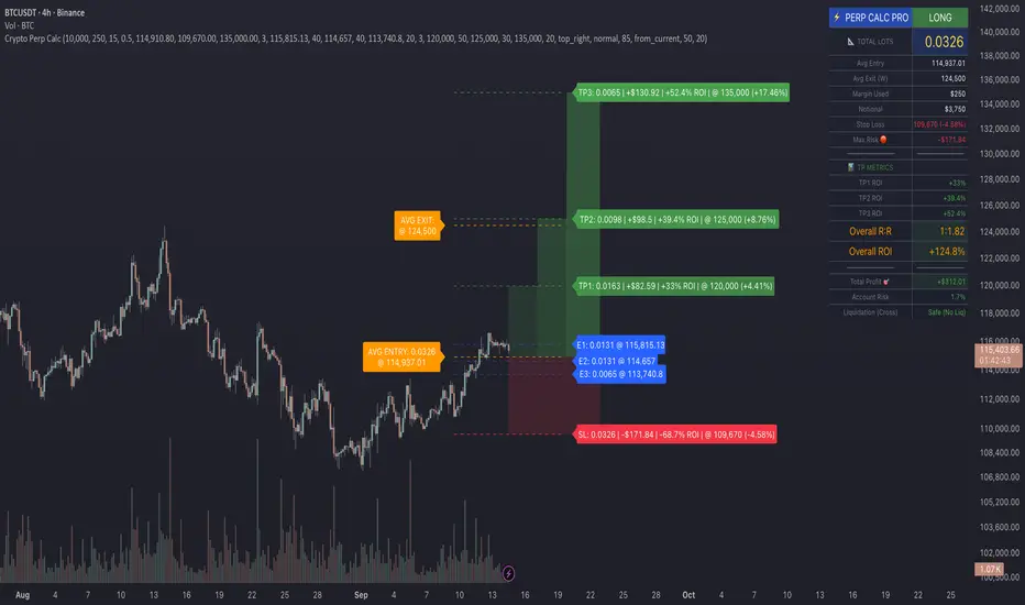
Multi Channel GRID & DCA LTF [trade_lexx]Multi Channel GRID & DCA LTF
Usage Guide
Part 1: The concept and general possibilities of the "Multi Channel GRID & DCA LTF" strategy
Introduction
Welcome to the guide to "Multi Channel GRID & DCA LTF", a powerful and versatile automated trading strategy for the TradingView platform. This tool was developed for traders who are looking for flexibility, control and a high degree of adaptability to various market conditions.
The strategy is based on a hybrid approach that combines two popular and time-tested techniques.:
1. GRID (grid trading): The classic method of averaging a position is by placing a grid of limit orders.
2. DCA (Dollar Cost averaging): Smart position averaging based on signals from external indicators.
However, "Multi Channel GRID & DCA LTF" goes far beyond the simple combination of these two techniques. The strategy includes a number of unique and innovative features, such as cascading MultiGRID grids for dealing with extreme volatility, Channel Mode range trading mode for profiting from sideways movement, and Low Time Frame analysis (LTF) to achieve surgical accuracy in backtesting. Deep customization options for risk management, capital, take profits, and stop losses allow you to configure a strategy for almost any trading style, asset, and timeframe.
The basic idea: How does it work?
Let's take a detailed look at each of the key concepts embedded in the logic of the strategy.
1. GRID — Automatic placement of buy and sell orders at certain price intervals.
This is a fundamental mode of operation. Its main goal is to systematically improve the average entry price for a position if the market is going against you.
* The principle of operation: After opening the base (first) order (`BO`), the strategy automatically places a series of pending limit orders (here they are called "safety orders" or "SO") at certain price intervals. For a long position, orders are placed below the entry price, and for a short position, orders are placed higher.
* Target: When the price moves against an open position, it consistently hits and executes safety orders. Each such execution adds additional volume to the position at a more favorable price, thereby shifting the overall average entry price (`position_avg_price') closer to the current market price. This means that a much smaller corrective movement will be required to gain ground.
* Flexibility: You have full control over the geometry of the grid: the number of safety orders, the percentage distance between them (`SO Step`), and you can even set a coefficient that will increase this step for each subsequent order (`SO Multiplier`), creating an expanding grid.
2. DCA (Signal Averaging) — Smart Averaging
This mode adds an additional layer of analysis to the averaging process. Instead of just buying/selling at the set price levels, the strategy waits for a confirmation signal.
* Working principle: You can connect any external indicator (for example, RSI, CCI, or even your own complex signal system) to the strategy, which outputs numerical values. As standard, 1 is used for a long signal, and -1 is used for a short signal. The strategy will place the next averaging order only at the moment when it receives the appropriate signal.
* Goal: To average a position not just during a fall (or a rise for a short), but at the moments that your main trading system considers the most favorable for this. This allows you to avoid "catching falling knives" and enter only if there are good reasons.
3. Hybrid Mode (GRID+DCA) is the best of the previous two modes
This mode is designed for maximum filtering and control. It requires two conditions to be fulfilled simultaneously.
* Working principle: The safety order will be executed only if the price has reached the calculated grid level and a confirmation signal has been received from your external indicator. If a confirmation signal is received from an external indicator, the next calculated grid level activates the limit order.
* Goal: To create the most reliable averaging system that protects against premature entries and requires double confirmation (both by price and indicator) before increasing the position size.
4. MultiGRID — Adaptation to extreme volatility
This is one of the most powerful and unique features of a strategy designed to survive and make a profit in the face of strong, protracted trends or "black swans".
* The problem it solves: The usual grid of orders has a limited depth. If the price goes beyond the last safety order, the strategy loses the opportunity to average and becomes vulnerable.
* The principle of operation: The MultiGRID function allows you to create "cascades" — several grids following one another. When all the orders of the first grid are executed, the strategy does not stop. Instead, she can activate the second, third (and so on) a grid of orders. The new grid can be activated by one of two triggers:
1. Offset: The new grid is activated when the price passes another set percentage deviation from the last executed order.
2. Signal: The new grid is activated when a signal is received from an external indicator.
* Goal: To significantly expand the working range of the strategy. This allows it to adapt to strong market movements that would "break" the usual grid, and continue to effectively average a position at a much greater depth of decline or growth.
5. Channel Mode — Trading in the range
This feature turns a standard averaging strategy into a machine for "farming" profits within a price channel that is formed during a sideways market movement.
* The problem it solves: In the standard grid strategy, after partially closing a take profit position, the volume of this part "leaves" the trade until the deal is fully closed. You are missing the opportunity to reuse this capital.
* Operating principle: When Channel Mode is enabled, the following happens. Suppose the price went against you, executed several safety orders, and then turned around and reached one of the partial take profits. At this point, the strategy is:
1. Fixes the profit, as it should be.
2. Instantly places a new limit order to buy (or sell for a short) at exactly the same price level where the last triggered safety order was executed. The volume of this order is equal to the volume of the part that was just closed for take profit.
3. If the price goes down again and executes this "repeat" order, the strategy immediately sets a corresponding take profit for it at the level where the previous profit was taken.
* Goal: To create a continuous buy-sell cycle within the local range (channel). The lower limit of the channel is the price of the last averaging, and the upper limit is the price of a partial take profit. This allows you to repeatedly profit from sideways price fluctuations, without waiting for the full closure of the main, large transaction.
6. LTF (Lower Timeframe Analysis) — Surgical precision of backtesting
This feature is critically important for obtaining reliable results during historical testing (backtesting) of grid strategies.
* The problem it solves: The standard testing mechanism in TradingView has a serious limitation. Working, for example, on a 4-hour chart, he sees only 4 candle points: Open, High, Low and Close. He does not know in what order the price moved within these 4 hours. He could have touched High first and then Low, or vice versa. For grid strategies, this is fatal — the engine can show that a take profit has been executed, although in reality the price first went down, collected the entire grid of orders and only then turned around.
* How it works: When you turn on the LTF mode, the strategy for each candle on your main chart (for example, 4H) requests and analyzes all candles from the lower timeframe you specified (for example, 1-minute). Then it virtually trades the entire price path for these minute candles, executing orders, take profits and stop losses in the sequence in which they would occur in reality. It works in the single take profit mode of the Grid strategy.
* Goal: To provide the most realistic and reliable backtest that reflects the real dynamics of the market. This allows you to avoid false expectations and accurately assess the potential performance of the strategy.
// ------------------------
Part 2: Detailed description of the strategy settings
This section is your main guide to all the switches and options available in the strategy. Understanding each setting is the key to unlocking the full potential of this powerful tool.
1. 🛡️ Risk Management 🛡️
This group contains fundamental parameters that determine the basic logic of risk management and the geometry of grid orders.
* Strategy type: Determines the direction of transactions.
* Long: The strategy will only open long positions (buy).
* Short: The strategy will only open short positions (sell).
* Both: The strategy will work both ways, opening long or short depending on the incoming signal.
* SO Count: Sets the maximum number of Safety (averaging) Orders (SO) that the strategy will place within the same grid. If you have MultiGRID enabled, this number applies to each individual grid.
* SO Step (%): This is the base percentage deviation from the entry price at which the first safety order will be placed. For example, at a value of 0.5, the first SO in a long trade will be placed 0.5% lower than the opening price of the base order.
* SO Multiplier: A coefficient that exponentially increases the step for each subsequent safety order. This allows you to create an expanding grid where averaging orders are placed further and further apart, which is effective with strong and accelerating price movements.
* *The step formula for the nth order*: Step(N) = (SO Step) * (SO Multiplier ^(N-1)).
* If the value is 1, all steps will be the same.
* With a value of 1.6, the step of the second SO will be 1.6 times larger than the first, the step of the third will be 1.6 times larger than the second, and so on.
* 1️⃣ TP/SL: These are simplified settings for quick configuration. They allow you to turn on/off the main take profit and stop loss and set basic percentage values for them. More detailed settings for these parameters can be found in the relevant sections below.
// ------------------------
2. 💰 Money Management 💰
Everything related to position size, leverage, and capital is configured here.
* Volume BO (Base Order): Determines the size of the trade's opening order.
* Volume BO: A fixed amount in the quote currency (for example, in USDT).
* USDT (check mark): Manages the information in the comments to the orders. If enabled, the volume of orders in USDT will be displayed in the comments. This is convenient for visual analysis and for sending the amount of USDT by the placeholder {{strategy.order.comment}} via webhooks when connecting the strategy to the exchange or trading terminals.
* or % of deposit: The amount calculated as a percentage of the available capital of the strategy. The check mark to the right of this field enables this mode. Important: using a percentage activates the effect of compounding (compound interest), as the amount of each new transaction will be automatically recalculated based on the current capital (initial capital + profit/loss). If enabled, the percentage of orders will be displayed in the comments. This is convenient for visual analysis and for sending percentages on the placeholder {{strategy.order.comment}} via webhooks when connecting the strategy to the stock exchange, trading terminals, or creating Copy trading.
* Martingale: The coefficient applied to the volume of orders. It increases the size of each subsequent insurance order compared to the base one.
* Volume formula for the nth SO: Volume SO (N) = (Volume BO) * (Martingale^N).
* With a value of 1.2, the volume of the first SO will be 1.2 times greater than the base, the second — 1.44 times (`1.2 * 1.2`) and so on.
* Leverage: Specify the size of your leverage. This parameter is used exclusively for calculating and displaying the approximate liquidation price. It does not affect the size of positions, but it helps to visually assess the risks.
* Liquidation: Enables or disables the calculation and display of the liquidation line on the chart.
* Margin type: Allows you to select a method for calculating the liquidation price, simulating the logic of exchanges:
* Isolated: The liquidation price is calculated based on the size and leverage of the current open position only.
* Cross: The calculation simulates using the entire available balance to maintain a position. In the strategy, the liquidation price is calculated as the level at which the loss on the current transaction is equal to the current capital.
* Commission (%): Specify the percentage of your exchange's commission per transaction. The correct value of this parameter is crucial for obtaining realistic backtest results.
// ------------------------
3. 🕸️ Grid Management 🕸️
This group is responsible for the logic of safety orders and advanced mechanics such as Channel Mode and MultiGRID.
* SO Type: Defines the logic of placing averaging orders.
* GRID: Classic grid. All safety orders are placed in advance as limit orders.
* DCA: Signal averaging. The strategy is waiting for a signal from an external indicator to place a market averaging order.
* GRID+DCA: Hybrid. The strategy waits for a signal, and if it arrives, places a limit order at the appropriate price level of the grid or executes a market order if the signal has arrived below the limit order level.
* Signal for SO: A data source (indicator) that will be used for signals in DCA and GRID+DCA modes.
* ↔️ Channel Mode: When this option is enabled, the strategy tries to trade in a sideways range. After partially closing a take profit position, it immediately places a limit order for re-entry at the price of the last triggered safety order. This creates a buy-sell cycle within the local channel.
* Best Price Only: This filter adds an additional condition for averaging in DCA and MultiGRID modes (when it operates on a signal). The next averaging order or a new grid will be activated only if the current price is more favorable (lower for long, higher for short) than the price of the previous entry.
* 🧩 MultiGRID ⮕ Enables cascading grid mode.
* Grid Count: The total number of grids that can be activated sequentially.
* Offset: Percentage deviation from the price of the last order of the previous grid. When this margin is reached, the following grid of orders is activated (this mode does not require a signal).
* Or signal: Allows you to use the signal from an external indicator as a trigger to activate the next grid. The checkmark on the right turns on this mode.
// ------------------------
4. 🎯 Entry and Stop 🎯
This group of settings allows you to fine-tune the conditions for starting a new trade and all aspects related to protective stop orders, including the complex mechanics of trailing and managing SL after partial take profits.
* 🎯 Signal: A data source (indicator) that will be used to determine when to enter a trade. The strategy expects a value of 1 for the start of a long trade and -1 for a short trade.
* Min Bars: Sets the minimum number of candles that must pass from the moment of opening the previous trade to the moment of opening the next one. A value of 0 disables this filter. This is a useful tool to prevent overly frequent entries in a "noisy" market.
* Non-stop: If this option is enabled, the strategy ignores the Entry Signal and opens a new trade immediately after closing the previous one (taking into account the Min Bars filter, if it is set). This turns the strategy into a constantly working mechanism that is always on the market.
* 🛑 SL Type: Defines the base price from which the stop loss percentage will be calculated. The stop loss in the first section must be enabled for this block of settings to work.
* From the entry point: SL is always calculated from the opening price of the very first base order. It remains static throughout the entire transaction unless it is moved by other functions.
* From breakeven line: SL is dynamically recalculated and shifted each time a safety order is executed. It always follows the average price of the position, being at a given percentage distance from it.
* From last executed SO: SL is recalculated from the price of the last executed order, whether it is a base or a safety order.
* From last SO: SL is calculated from the price of the most recent possible safety order in the grid. This is usually the most remote and conservative type of SL.
* Trailing SL Type: Defines the algorithm by which the stop loss will move after its activation.
* Standard: Classic trailing. After activation, SL will follow the price at a fixed distance.
* ATR: SL will follow the price at a distance equal to the value of the ATR indicator multiplied by the specified multiplier.
* External Source: SL will follow any selected line of the third-party indicator.
* Period and Multiplier: Common parameters for all types of trailing.
* Source: The source of the line for the trailing SL of the third-party indicator.
* Trailing SL after entry: The mode of activation of the trailing SL after entering the transaction
* SL management after TP (sections 1️⃣, 2️⃣, 3️⃣): These three blocks allow you to create a complex stop loss management logic as profits are recorded.
For each take profit level (TP1, TP2, TP3), you can configure:
* SL BE / SL TP1 / SL TP2: When the corresponding TP is reached, the stop loss will be moved to the breakeven point (for TP1), to the TP1 price level (for TP2) or to the TP2 price level (for TP3).
* Trailing SL: When the corresponding TP is reached, the trailing stop loss is activated according to the settings above.
* By ↔️ Signal: A very powerful option. If it is enabled, the above action (SL transfer or trailing activation) will occur when the opposite trading signal is received from an external indicator. This allows you to protect profits or reduce losses if the market turns sharply, even before reaching the target.
* SL Delay ⮕ Allows you to delay the activation of the stop loss.
* Number of Bars: The Stop loss will be physically placed on the market only after the specified number of candles has passed since entering the trade. This can help to avoid "taking out" the stop with a random short movement (squiz) immediately after opening a position.
* SL Block: Unique defensive mechanics for trading both ways (`Strategy Type: Both`).
* Number of SL: If the strategy receives the specified number of stop losses in a row in one direction (for example, 2 stops long), it temporarily blocks the opportunity to open new trades in that direction.
* Lock Reset mode:
* By direction: The lock is lifted if a profitable trade is closed in the allowed direction or if a stop loss is triggered in the opposite direction.
* First profit: The lock is lifted after closing any profitable transaction, regardless of its direction.
// ------------------------
5. ✅ Take Profit ✅
This group of settings provides comprehensive control over profit taking, from a simple take profit to a complex system of partial closures and trailing.
* ✅ TP Type: Defines the base price for calculating the percentage deviation of the take profit.
* From entry point: TP is calculated from the base order price.
* From breakeven line: TP dynamically follows the average position price.
* From last executed SO: TP is calculated from the price of the last executed order.
* Filters for closing on signal
* Only ➕: If TP is triggered by a signal, the deal will be closed only if it is in the black relative to the average price.
* Or >TP: If TP is triggered by a signal, the trade will be closed only if the closing price is better than (or equal to) the estimated price of this TP.
* TP type of trailing: Yes, take profit has a trailing too! It works differently than the SL trailing.
* Standard / ATR: After the price touches the "virtual" TP level, the trailing is activated. He does not place a stop order, but begins to move away from the price, dynamically moving the limit order to close further and further in the profitable direction, allowing him to collect the maximum from the impulse movement.
* External Source: TP will follow any selected line of the third-party indicator.
* Period and Multiplier: Parameters for calculating the trailing margin TP.
* Source: The source of the line for the trailing TP of the third-party indicator.
* TP level settings (sections 1️⃣, 2️⃣, 3️⃣, 4️⃣): The strategy supports up to four independent take profit levels, which allows for a flexible system of partial commits.
For each level, you can set:
* TP: Enable the level and set its percentage deviation from the base price.
* Size: What percentage of the current position will be closed when this level is reached. For the last active TP, this parameter is ignored, and 100% of the remaining position is closed.
* Trailing TP: Enable the above-described trailing mechanism for this particular level.
* Signal: Enable closing based on the signal from the external indicator for this level.
* Or take: If both the closing on the signal and the limit order are enabled, then whatever comes first will work.
* After SO: Activate this TP level only after the specified number of safety orders has been executed. This allows you to set closer targets for riskier (deeply averaged) positions.
// ------------------------
6. 🔬 GRID and MultiGrid Analysis on Lower TFs (LTF) 🔬
This group activates one of the most important functions for accurate testing of grid strategies.
* Enable LTF Calculation ⮕ The main switch of the analysis mode on the lower timeframes.
* Timeframe selection: A drop-down list where you can select a timeframe for detailed analysis. For example, if your main schedule is 1 hour, you can select 1 minute here. The strategy will emulate the trading of minute candles within each hour candle.
❗️Important: As mentioned in the first part, the use of this mode is critically necessary to obtain realistic backtest results, especially for strategies with a dense grid of orders. Without it, the results may be overly optimistic and not reflect the real dynamics of the market. It should be remembered that TradingView imposes a limit on the number of intra-bars (minor TF bars) that can be requested. This is usually about 100,000 bars.
// ------------------------
7. 🕘 Backtest Date Range 🕘
This group allows you to focus testing on a specific historical period.
* Limit Date Range: Enables date filtering.
* Start time: The date and time when the strategy will start analyzing and opening deals.
* End time: The date and time after which the strategy will stop opening new deals and complete testing.
// ------------------------
8. 🎨 Visualization 🎨
All the options responsible for the appearance and information content of the chart are collected here.
* Show PnL labels: Enables/disables the display of text labels with the result (profit/loss) after closing each trade.
* Statistics Table: Enables/disables the main dashboard with detailed statistics on the results of the backtest.
* Strategy Settings Table: Enables/disables an additional panel that summarizes all the key parameters of the current configuration.
* Monthly Profit Table: Enables/disables a table with a breakdown of percentage returns by month and year.
* Table settings: For each of the three tables, you can individually adjust the Text size and Table Position on the screen to position them as conveniently as possible.
* Decimal places: Defines how many decimal places will be displayed in numeric values in tables and on labels.
// ------------------------
9. ✉️ Webhook Settings ✉️
This group is intended for traders who want to automate trading on strategy signals using third-party services and exchanges (for example, 3Commas, WunderTrading, Cryptorobotics, Cryptohopper, Bitsgap, Binance, ByBit, OKX, Pionex, Bitget or proprietary solutions).
For each key event in the strategy, there is a separate switch and a text field:
* Webhook for Open: Enable and set a message for the webhook that will be sent when the base order is opened.
* Webhook for Averaging: A message sent when executing any insurance order.
* Webhook for Take Profit: A message sent when closing on take profit (including partial ones).
* Webhook for Stop-Loss: A message sent when a stop loss is closed.
You can insert a JSON code or any other message format that your service requires for automation into the text fields. The strategy supports special placeholders (for example, `{{strategy.order.alert_message}}`), which allow you to dynamically insert the necessary data into the message, such as the amount of USDT or the percentage of the deposit for entry, averaging and take profit orders.

Adaptive MVRV & RSI Strategy V6 (Dynamic Thresholds)Strategy Explanation
This is an advanced Dollar-Cost Averaging (DCA) strategy for Bitcoin that aims to adapt to long-term market cycles and changing volatility. Instead of relying on fixed buy/sell signals, it uses a dynamic, weighted approach based on a combination of on-chain data and classic momentum.
Core Components:
Dual-Indicator Signal: The strategy combines two powerful indicators for a more robust signal:
MVRV Ratio: An on-chain metric to identify when Bitcoin is fundamentally over or undervalued relative to its historical cost basis.
Weekly RSI: A classic momentum indicator to gauge long-term market strength and identify overbought/oversold conditions.
Dynamic, Self-Adjusting Thresholds: The core innovation of this strategy is that it avoids fixed thresholds (e.g., "sell when RSI is 70"). Instead, the buy and sell zones are dynamically calculated based on a long-term (2-year) moving average and standard deviation of each indicator. This allows the strategy to automatically adapt to Bitcoin's decreasing volatility and changing market structure over time.
Weighted DCA (Scaling In & Out): The strategy doesn't just buy or sell a fixed amount. The size of its trades is scaled based on conviction:
Buying: As the MVRV and RSI fall deeper into their "undervalued" zones, the percentage of available cash used for each purchase increases.
Selling: As the indicators rise further into "overvalued" territory, the percentage of the current position sold also increases.
This creates an adaptive system that systematically accumulates during periods of fear and distributes during periods of euphoria, with the intensity of its actions directly tied to the extremity of market conditions.

Dynamic DCA Envelope – Beta V1.1Dynamic DCA Envelope-Beta V1.1 is a preview version of a Dollar-Cost Averaging (DCA) strategy designed for trending or volatile markets.
-Long Positions Only
-Intended for Cryptocurrency, but can be used in any market
-1 and 4 hour timeframe
-Average Commissions 0.1%-0.3% per trade (Cryptocurrency)
What it does:
This strategy identifies buying opportunities when price closes below a dynamic envelope (based on EMA). After 3 consecutive closes below the lower envelope, the system arms a buy condition. A DCA buy-in is triggered when price bounces by a configurable percentage from the trailing low. The strategy supports up to 3 buy-ins, each equally sized, and closes the entire position at a fixed take profit or stop loss.
How it works:
-Entry logic is based on price deviation from an EMA envelope
-Waits for 3 closes below the envelope to detect weakness
-Uses bounce percentage from the lowest point to trigger each buy
-Includes cooldown logic between buys to avoid clustering
-All positions are closed when TP or SL is hit
How to use it:
-Use on trending assets with volatility (e.g., crypto, tech stocks)
-Adjust inputs to match asset behavior:
-EMA Length
-Envelope Offset %
-Bounce % (Trailing DCA)
-Take Profit / Stop Loss
-View strategy performance in the Strategy Tester tab
What’s unique:
Unlike most DCA scripts that immediately average down, this version includes:
-Trigger logic requiring multiple closes below trend
-Bounce-based entry to avoid catching a falling knife
-Cooldown resets to prevent overtrading
-A true entry–wait–buy–reset loop mimicking disciplined execution
*This is a beta version intended as a preview. A full Pro version is in development, which includes:
-SmartScaling logic
-Trailing take profit
-Multi-symbol scanning
-Backtest range limits
-Risk-adjusted filtering
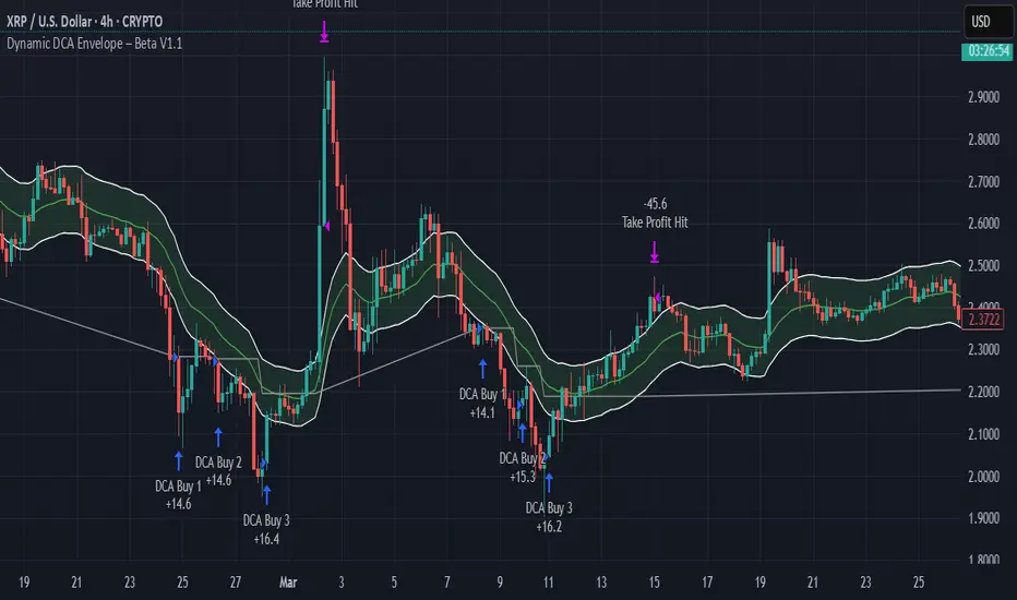
Ticker Pulse Meter BasicPairs nicely with the Contrarian 100 MA located here:
and the Enhanced Stock Ticker with 50MA vs 200MA located here:
Description
The Ticker Pulse Meter Basic is a dynamic Pine Script v6 indicator designed to provide traders with a visual representation of a stock’s price position relative to its short-term and long-term ranges, enabling clear entry and exit signals for long-only trading strategies. By calculating three normalized metrics—Percent Above Long & Above Short, Percent Above Long & Below Short, and Percent Below Long & Below Short—this indicator offers a unique "pulse" of market sentiment, plotted as stacked area charts in a separate pane. With customizable lookback periods, thresholds, and signal plotting options, it empowers traders to identify optimal entry points and profit-taking levels. The indicator leverages Pine Script’s force_overlay feature to plot signals on either the main price chart or the indicator pane, making it versatile for various trading styles.
Key Features
Pulse Meter Metrics:
Computes three percentages based on short-term (default: 50 bars) and long-term (default: 200 bars) lookback periods:
Percent Above Long & Above Short: Measures price strength when above both short and long ranges (green area).
Percent Above Long & Below Short: Indicates mixed momentum (orange area).
Percent Below Long & Below Short: Signals weakness when below both ranges (red area).
Flexible Signal Plotting:
Toggle between plotting entry (blue dots) and exit (white dots) signals on the main price chart (location.abovebar/belowbar) or in the indicator pane (location.top/bottom) using the Plot Signals on Main Chart option.
Entry/Exit Logic:
Long Entry: Triggered when Percent Above Long & Above Short crosses above the high threshold (default: 20%) and Percent Below Long & Below Short is below the low threshold (default: 40%).
Long Exit: Triggered when Percent Above Long & Above Short crosses above the profit-taking level (default: 95%).
Visual Enhancements:
Plots stacked area charts with semi-transparent colors (green, orange, red) for intuitive trend analysis.
Displays threshold lines for entry (high/low) and profit-taking levels.
Includes a ticker and timeframe table in the top-right corner for quick reference.
Alert Conditions: Supports alerts for long entry and exit signals, integrable with TradingView’s alert system for automated trading.
Technical Innovation: Combines normalized price metrics with Pine Script v6’s force_overlay for seamless signal integration on the price chart or indicator pane.
Technical Details
Calculation Logic:
Uses confirmed bars (barstate.isconfirmed) to calculate metrics, ensuring reliability.
Short-term percentage: (close - lowest(low, lookback_short)) / (highest(high, lookback_short) - lowest(low, lookback_short)).
Long-term percentage: (close - lowest(low, lookback_long)) / (highest(high, lookback_long) - lowest(low, lookback_long)).
Derived metrics:
pct_above_long_above_short = (pct_above_long * pct_above_short) * 100.
pct_above_long_below_short = (pct_above_long * (1 - pct_above_short)) * 100.
pct_below_long_below_short = ((1 - pct_above_long) * (1 - pct_above_short)) * 100.
Signal Plotting:
Entry signals (long_entry) use ta.crossover to detect when pct_above_long_above_short crosses above entryThresholdhigh and pct_below_long_below_short is below entryThresholdlow.
Exit signals (long_exit) use ta.crossover for pct_above_long_above_short crossing above profitTake.
Signals are plotted as tiny circles with force_overlay=true for main chart or standard plotting for the indicator pane.
Performance Considerations: Optimized for efficiency by calculating metrics only on confirmed bars and using lightweight plotting functions.
How to Use
Add to Chart:
Copy the script into TradingView’s Pine Editor and apply it to your chart.
Configure Settings:
Short Lookback Period: Adjust the short-term lookback (default: 50 bars) for sensitivity.
Long Lookback Period: Set the long-term lookback (default: 200 bars) for broader context.
Entry Thresholds: Modify high (default: 20%) and low (default: 40%) thresholds for entry conditions.
Profit Take Level: Set the exit threshold (default: 95%) for profit-taking.
Plot Signals on Main Chart: Check to display signals on the price chart; uncheck for the indicator pane.
Interpret Signals:
Long Entry: Blue dots indicate a strong bullish setup when price is high relative to both lookback ranges and weakness is low.
Long Exit: White dots signal profit-taking when strength reaches overbought levels.
Use the stacked area charts to assess trend strength and momentum.
Set Alerts:
Create alerts for Long Entry and Long Exit conditions using TradingView’s alert system.
Customize Visuals:
Adjust colors and thresholds via TradingView’s settings for better visibility.
The ticker table displays the symbol and timeframe in the top-right corner.
Example Use Cases
Swing Trading: Use entry signals to capture short-term bullish moves within a broader uptrend, exiting at profit-taking levels.
Trend Confirmation: Monitor the green area (Percent Above Long & Above Short) for sustained bullish momentum.
Market Sentiment Analysis: Use the stacked areas to gauge bullish vs. bearish sentiment across timeframes.
Notes
Testing: Backtest the indicator on your chosen market and timeframe to validate its effectiveness.
Compatibility: Built for Pine Script v6 and tested on TradingView as of June 20, 2025.
Limitations: Signals are long-only; adapt the script for short strategies if needed.
Enhancements: Consider adding a histogram for the difference between metrics or additional thresholds for nuanced trading.
Acknowledgments
Inspired by public Pine Script examples and designed to simplify complex market dynamics into a clear, actionable tool. For licensing or support, contact Chuck Schultz (@chuckaschultz) on TradingView. Share feedback in the comments, and happy trading!

DCA Investment Tracker Pro [tradeviZion]DCA Investment Tracker Pro: Educational DCA Analysis Tool
An educational indicator that helps analyze Dollar-Cost Averaging strategies by comparing actual performance with historical data calculations.
---
💡 Why I Created This Indicator
As someone who practices Dollar-Cost Averaging, I was frustrated with constantly switching between spreadsheets, calculators, and charts just to understand how my investments were really performing. I wanted to see everything in one place - my actual performance, what I should expect based on historical data, and most importantly, visualize where my strategy could take me over the long term .
What really motivated me was watching friends and family underestimate the incredible power of consistent investing. When Napoleon Bonaparte first learned about compound interest, he reportedly exclaimed "I wonder it has not swallowed the world" - and he was right! Yet most people can't visualize how their $500 monthly contributions today could become substantial wealth decades later.
Traditional DCA tracking tools exist, but they share similar limitations:
Require manual data entry and complex spreadsheets
Use fixed assumptions that don't reflect real market behavior
Can't show future projections overlaid on actual price charts
Lose the visual context of what's happening in the market
Make compound growth feel abstract rather than tangible
I wanted to create something different - a tool that automatically analyzes real market history, detects volatility periods, and shows you both current performance AND educational projections based on historical patterns right on your TradingView charts. As Warren Buffett said: "Someone's sitting in the shade today because someone planted a tree a long time ago." This tool helps you visualize your financial tree growing over time.
This isn't just another calculator - it's a visualization tool that makes the magic of compound growth impossible to ignore.
---
🎯 What This Indicator Does
This educational indicator provides DCA analysis tools. Users can input investment scenarios to study:
Theoretical Performance: Educational calculations based on historical return data
Comparative Analysis: Study differences between actual and theoretical scenarios
Historical Projections: Theoretical projections for educational analysis (not predictions)
Performance Metrics: CAGR, ROI, and other analytical metrics for study
Historical Analysis: Calculates historical return data for reference purposes
---
🚀 Key Features
Volatility-Adjusted Historical Return Calculation
Analyzes 3-20 years of actual price data for any symbol
Automatically detects high-volatility stocks (meme stocks, growth stocks)
Uses median returns for volatile stocks, standard CAGR for stable stocks
Provides conservative estimates when extreme outlier years are detected
Smart fallback to manual percentages when data insufficient
Customizable Performance Dashboard
Educational DCA performance analysis with compound growth calculations
Customizable table sizing (Tiny to Huge text options)
9 positioning options (Top/Middle/Bottom + Left/Center/Right)
Theme-adaptive colors (automatically adjusts to dark/light mode)
Multiple display layout options
Future Projection System
Visual future growth projections
Timeframe-aware calculations (Daily/Weekly/Monthly charts)
1-30 year projection options
Shows projected portfolio value and total investment amounts
Investment Insights
Performance vs benchmark comparison
ROI from initial investment tracking
Monthly average return analysis
Investment milestone alerts (25%, 50%, 100% gains)
Contribution tracking and next milestone indicators
---
📊 Step-by-Step Setup Guide
1. Investment Settings 💰
Initial Investment: Enter your starting lump sum (e.g., $60,000)
Monthly Contribution: Set your regular DCA amount (e.g., $500/month)
Return Calculation: Choose "Auto (Stock History)" for real data or "Manual" for fixed %
Historical Period: Select 3-20 years for auto calculations (default: 10 years)
Start Year: When you began investing (e.g., 2020)
Current Portfolio Value: Your actual portfolio worth today (e.g., $150,000)
2. Display Settings 📊
Table Sizes: Choose from Tiny, Small, Normal, Large, or Huge
Table Positions: 9 options - Top/Middle/Bottom + Left/Center/Right
Visibility Toggles: Show/hide Main Table and Stats Table independently
3. Future Projection 🔮
Enable Projections: Toggle on to see future growth visualization
Projection Years: Set 1-30 years ahead for analysis
Live Example - NASDAQ:META Analysis:
Settings shown: $60K initial + $500/month + Auto calculation + 10-year history + 2020 start + $150K current value
---
🔬 Pine Script Code Examples
Core DCA Calculations:
// Calculate total invested over time
months_elapsed = (year - start_year) * 12 + month - 1
total_invested = initial_investment + (monthly_contribution * months_elapsed)
// Compound growth formula for initial investment
theoretical_initial_growth = initial_investment * math.pow(1 + annual_return, years_elapsed)
// Future Value of Annuity for monthly contributions
monthly_rate = annual_return / 12
fv_contributions = monthly_contribution * ((math.pow(1 + monthly_rate, months_elapsed) - 1) / monthly_rate)
// Total expected value
theoretical_total = theoretical_initial_growth + fv_contributions
Volatility Detection Logic:
// Detect extreme years for volatility adjustment
extreme_years = 0
for i = 1 to historical_years
yearly_return = ((price_current / price_i_years_ago) - 1) * 100
if yearly_return > 100 or yearly_return < -50
extreme_years += 1
// Use median approach for high volatility stocks
high_volatility = (extreme_years / historical_years) > 0.2
calculated_return = high_volatility ? median_of_returns : standard_cagr
Performance Metrics:
// Calculate key performance indicators
absolute_gain = actual_value - total_invested
total_return_pct = (absolute_gain / total_invested) * 100
roi_initial = ((actual_value - initial_investment) / initial_investment) * 100
cagr = (math.pow(actual_value / initial_investment, 1 / years_elapsed) - 1) * 100
---
📊 Real-World Examples
See the indicator in action across different investment types:
Stable Index Investments:
AMEX:SPY (SPDR S&P 500) - Shows steady compound growth with standard CAGR calculations
Classic DCA success story: $60K initial + $500/month starting 2020. The indicator shows SPY's historical 10%+ returns, demonstrating how consistent broad market investing builds wealth over time. Notice the smooth theoretical growth line vs actual performance tracking.
MIL:VUAA (Vanguard S&P 500 UCITS) - Shows both data limitation and solution approaches
Data limitation example: VUAA shows "Manual (Auto Failed)" and "No Data" when default 10-year historical setting exceeds available data. The indicator gracefully falls back to manual percentage input while maintaining all DCA calculations and projections.
MIL:VUAA (Vanguard S&P 500 UCITS) - European ETF with successful 5-year auto calculation
Solution demonstration: By adjusting historical period to 5 years (matching available data), VUAA auto calculation works perfectly. Shows how users can optimize settings for newer assets. European market exposure with EUR denomination, demonstrating DCA effectiveness across different markets and currencies.
NYSE:BRK.B (Berkshire Hathaway) - Quality value investment with Warren Buffett's proven track record
Value investing approach: Berkshire Hathaway's legendary performance through DCA lens. The indicator demonstrates how quality companies compound wealth over decades. Lower volatility than tech stocks = standard CAGR calculations used.
High-Volatility Growth Stocks:
NASDAQ:NVDA (NVIDIA Corporation) - Demonstrates volatility-adjusted calculations for extreme price swings
High-volatility example: NVIDIA's explosive AI boom creates extreme years that trigger volatility detection. The indicator automatically switches to "Median (High Vol): 50%" calculations for conservative projections, protecting against unrealistic future estimates based on outlier performance periods.
NASDAQ:TSLA (Tesla) - Shows how 10-year analysis can stabilize volatile tech stocks
Stable long-term growth: Despite Tesla's reputation for volatility, the 10-year historical analysis (34.8% CAGR) shows consistent enough performance that volatility detection doesn't trigger. Demonstrates how longer timeframes can smooth out extreme periods for more reliable projections.
NASDAQ:META (Meta Platforms) - Shows stable tech stock analysis using standard CAGR calculations
Tech stock with stable growth: Despite being a tech stock and experiencing the 2022 crash, META's 10-year history shows consistent enough performance (23.98% CAGR) that volatility detection doesn't trigger. The indicator uses standard CAGR calculations, demonstrating how not all tech stocks require conservative median adjustments.
Notice how the indicator automatically detects high-volatility periods and switches to median-based calculations for more conservative projections, while stable investments use standard CAGR methods.
---
📈 Performance Metrics Explained
Current Portfolio Value: Your actual investment worth today
Expected Value: What you should have based on historical returns (Auto) or your target return (Manual)
Total Invested: Your actual money invested (initial + all monthly contributions)
Total Gains/Loss: Absolute dollar difference between current value and total invested
Total Return %: Percentage gain/loss on your total invested amount
ROI from Initial Investment: How your starting lump sum has performed
CAGR: Compound Annual Growth Rate of your initial investment (Note: This shows initial investment performance, not full DCA strategy)
vs Benchmark: How you're performing compared to the expected returns
---
⚠️ Important Notes & Limitations
Data Requirements: Auto mode requires sufficient historical data (minimum 3 years recommended)
CAGR Limitation: CAGR calculation is based on initial investment growth only, not the complete DCA strategy
Projection Accuracy: Future projections are theoretical and based on historical returns - actual results may vary
Timeframe Support: Works ONLY on Daily (1D), Weekly (1W), and Monthly (1M) charts - no other timeframes supported
Update Frequency: Update "Current Portfolio Value" regularly for accurate tracking
---
📚 Educational Use & Disclaimer
This analysis tool can be applied to various stock and ETF charts for educational study of DCA mathematical concepts and historical performance patterns.
Study Examples: Can be used with symbols like AMEX:SPY , NASDAQ:QQQ , AMEX:VTI , NASDAQ:AAPL , NASDAQ:MSFT , NASDAQ:GOOGL , NASDAQ:AMZN , NASDAQ:TSLA , NASDAQ:NVDA for learning purposes.
EDUCATIONAL DISCLAIMER: This indicator is a study tool for analyzing Dollar-Cost Averaging strategies. It does not provide investment advice, trading signals, or guarantees. All calculations are theoretical examples for educational purposes only. Past performance does not predict future results. Users should conduct their own research and consult qualified financial professionals before making any investment decisions.
---
© 2025 TradeVizion. All rights reserved.