AlphaMACD - Adaptive MACD with Efficiency RatioOVERVIEW
AlphaMACD is an adaptive implementation of the classic MACD indicator that dynamically adjusts its calculation periods based on market efficiency. Unlike traditional MACD which uses fixed periods (typically 12, 26, 9), this indicator adapts its fast and slow EMA periods in real-time based on how efficiently the market is trending.
WHAT MAKES THIS ORIGINAL
This is not a simple MACD with different settings or colors. The core innovation is the adaptive period calculation using Kaufman's Efficiency Ratio, which was originally developed for the Adaptive Moving Average (AMA). This indicator applies that adaptive logic to MACD itself.
Key Differences from Standard MACD:
- Periods dynamically adjust between user-defined ranges (default: 8-21 for fast, 21-55 for slow)
- Uses Kaufman's Efficiency Ratio to measure market trendiness
- Implements gap protection to prevent extreme spikes from market gaps
- Includes market regime detection to filter signals in choppy conditions
- Provides multi-timeframe trend confirmation
HOW IT WORKS
1. Efficiency Ratio Calculation:
The indicator calculates market efficiency by comparing the absolute price change over a period to the sum of absolute price changes within that period. High efficiency = strong trending market. Low efficiency = choppy/sideways market.
2. Adaptive Period Adjustment:
- In trending markets (high efficiency): Periods move toward the minimum values for faster response
- In choppy markets (low efficiency): Periods move toward the maximum values for slower, more stable signals
- The "Sensitivity" parameter controls how aggressively periods adapt (0.5 to 5.0)
3. Gap Protection:
The custom adaptive EMA function detects abnormal price gaps (moves larger than 3x the typical ATR-based change) and limits their impact on the calculation. This prevents weekends or news gaps from causing extreme MACD spikes.
4. Signal Quality Filtering:
- Market regime detection identifies trending vs sideways conditions
- Momentum filter (RSI-based) prevents signals during overextended moves
- Signal strength calculation helps identify high-confidence setups
- Sideways market signals are marked with warning symbols
5. Multi-Timeframe Analysis:
The indicator compares current timeframe MACD with a higher timeframe (default 60 min) to provide context and filter against-trend signals.
HOW TO USE IT
Settings:
- Core Settings: Define the minimum and maximum periods for fast/slow EMAs
- Sensitivity: Higher values make the indicator more responsive to market changes
- Multi-timeframe: Set a higher timeframe for trend confirmation
- Visual options: Customize appearance and enable/disable features
Signal Interpretation:
- Strong bullish/bearish signals (large triangles): High-confidence entries in trending markets
- Warning signals (small ⚠): Crossovers in sideways markets - use caution or skip
- Divergence labels ("DIV"): Price and MACD diverging - potential reversal
- Background color: Green tint = trending market, Orange tint = sideways market
The Information Table shows:
- Current market regime (trending or sideways)
- Market efficiency percentage (how clean the trend is)
- Current adaptive fast and slow periods
- Higher timeframe trend direction
- Current signal strength
Best Practices:
- In trending markets: Trust strong signals, avoid warning signals
- In sideways markets: Reduce position sizes or skip trades entirely
- Use higher timeframe confirmation for better signal quality
- Adjust sensitivity based on your trading timeframe (higher for intraday, lower for swing)
TECHNICAL DETAILS
Calculation Method:
- Efficiency Ratio = ABS(Close - Close ) / SUM(ABS(Close - Close ), Period)
- Smoothed Efficiency = EMA(Efficiency Ratio, 5)
- Fast Period = Fast_Min + (Fast_Max - Fast_Min) × (1 - Smoothed_Efficiency × Sensitivity)
- Slow Period = Slow_Min + (Slow_Max - Slow_Min) × (1 - Smoothed_Efficiency × Sensitivity)
- Adaptive EMA uses standard EMA formula with gap detection and limiting
- MACD = Fast Adaptive EMA - Slow Adaptive EMA
- Signal = EMA(MACD, Signal Period)
- Histogram = MACD - Signal
The adaptive periods are calculated on every bar, so the MACD responds faster in trending conditions and stabilizes during consolidation.
WHAT THIS SOLVES
Standard MACD Problems:
- Fixed periods don't adapt to changing market conditions
- Too many false signals in sideways markets
- Whipsaws during low-volatility consolidation
- Price gaps can cause misleading spikes
AlphaMACD Solutions:
- Periods automatically adjust to market state
- Market regime filter identifies and warns about sideways conditions
- Adaptive smoothing reduces whipsaws
- Gap protection prevents false extremes
LIMITATIONS
- Like all indicators, this does not predict the future
- Requires trending markets for optimal performance
- Adaptive calculation means backtesting results will differ from fixed-period MACD
- More complex than standard MACD - requires understanding of adaptive concepts
- The adaptive periods mean you cannot directly compare this to traditional MACD studies
This indicator is best used as part of a complete trading system, not as a standalone signal generator.
EDUCATIONAL VALUE
For traders learning about:
- Adaptive indicators and market efficiency concepts
- Kaufman's Adaptive Moving Average principles applied to oscillators
- Market regime detection and signal filtering
- Gap handling in technical indicators
- Multi-timeframe analysis integration
Not Financial advice.
Adaptive

Adaptive Vol Gauge [ParadoxAlgo]This is an overlay tool that measures and shows market ups and downs (volatility) based on daily high and low prices. It adjusts automatically to recent price changes and highlights calm or wild market periods. It colors the chart background and bars in shades of blue to cyan, with optional small labels for changes in market mood. Use it for info only—combine with your own analysis and risk controls. It's not a buy/sell signal or promise of results.Key FeaturesSmart Volatility Measure: Tracks price swings with a flexible time window that reacts to market speed.
Market Mood Detection: Spots high-energy (wild) or low-energy (calm) phases to help see shifts.
Visual Style: Uses smooth color fades on the background and bars—cyan for calm, deep blue for wild—to blend nicely on your chart.
Custom Options: Change settings like time periods, sensitivity, colors, and labels.
Chart Fit: Sits right on your main price chart without extra lines, keeping things clean.
How It WorksThe tool figures out volatility like this:Adjustment Factor:Looks at recent price ranges compared to longer ones.
Tweaks the time window (between 10-50 bars) based on how fast prices are moving.
Volatility Calc:Adds up logs of high/low ranges over the adjusted window.
Takes the square root for the final value.
Can scale it to yearly terms for easy comparison across chart timeframes.
Mood Check:Compares current volatility to its recent average and spread.
Flags "high" if above your set level, "low" if below.
Neutral in between.
This setup makes it quicker in busy markets and steadier in quiet ones.Settings You Can ChangeAdjust in the tool's menu:Base Time Window (default: 20): Starting point for calculations. Bigger numbers smooth things out but might miss quick changes.
Adjustment Strength (default: 0.5): How much it reacts to price speed. Low = steady; high = quick changes.
Yearly Scaling (default: on): Makes values comparable across short or long charts. Turn off for raw numbers.
Mood Sensitivity (default: 1.0): How strict for calling high/low moods. Low = more shifts; high = only big ones.
Show Labels (default: on): Adds tiny "High Vol" or "Low Vol" tags when moods change. They point up or down from bars.
Background Fade (default: 80): How see-through the color fill is (0 = invisible, 100 = solid).
Bar Fade (default: 50): How much color blends into your candles or bars (0 = none, 100 = full).
How to Read and Use ItColor Shifts:Background and bars fade based on mood strength:Cyan shades mean calm markets (good for steady, back-and-forth trades).
Deep blue shades mean wild markets (watch for big moves or turns).
Smooth changes show volatility building or easing.
Labels:"High Vol" (deep blue, from below bar): Start of wild phase.
"Low Vol" (cyan, from above bar): Start of calm phase.
Only shows at changes to avoid clutter. Use for timing strategy tweaks.
Trading Ideas:Mood-Based Plays: In wild phases (deep blue), try chase-momentum or breakout trades since swings are bigger. In calm phases (cyan), stick to bounce-back or range trades.
Risk Tips: Cut trade sizes in wild times to handle bigger losses. Use calm times for longer holds with close stops.
Chart Time Tips: Turn on yearly scaling for matching short and long views. Test settings on past data—loosen for quick trades (more alerts), tighten for longer ones (fewer, stronger).
Mix with Others: Add trend lines or averages—buy in calm up-moves, sell in wild down-moves. Check with volume or key levels too.
Special Cases: In big news events, it reacts faster. On slow assets, it might overstate swings—ease the adjustment strength.
Limits and TipsIt looks back at past data, so it trails real-time action and can't predict ahead.
Results differ by stock or timeframe—test on history first.
Colors and tags are just visuals; set your own alerts if needed.
Follows TradingView rules: No win promises, for learning only. Open for sharing; share thoughts in forums.
With this, you can spot market energy and tweak your trades smarter. Start on practice charts.

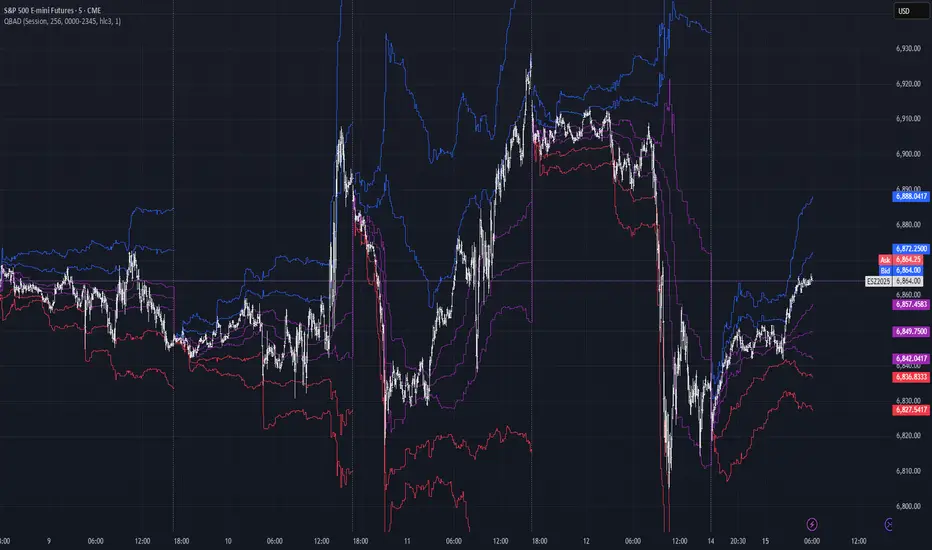
Quantile-Based Adaptive Detection🙏🏻 Dedicated to John Tukey. He invented the boxplot, and I finalized it.
QBAD (Quantile-Based Adaptive Detection) is ‘the’ adaptive (also optionally weighted = ready for timeseries) boxplot with more senseful fences. Instead of hardcoded multipliers for outer fences, I base em on a set of quantile-based asymmetry metrics (you can view it as an ‘algorithmic’ counter part of central & standardized moments). So outer bands are Not hardcoded, not optimized, not cross-validated etc, simply calculated at O(nlogn).
You can use it literally everywhere in any context with any continuous data, in any task that requires statistical control, novelty || outlier detection, without worrying and doubting the sense in arbitrary chosen thresholds. Obviously, given the robust nature of quantiles, it would fit best the cases where data has problems.
The thresholds are:
Basis: the model of the data (median in our case);
Deviations: represent typical spread around basis, together form “value” in general sense;
Extensions: estimate data’s extremums via combination of quantile-based asymmetry metrics without relying on actual blunt min and max, together form “range” / ”frame”. Datapoints outside the frame/range are novelties or outliers;
Limits: based also on quantile asymmetry metrics, estimate the bounds within which values can ‘ever’ emerge given the current data generating process stays the same, together form “field”. Datapoints outside the field are very rare, happen when a significant change/structural break happens in current data-generating process, or when a corrupt datapoint emerges.
…
The first part of the post is for locals xd, the second is for the wanderers/wizards/creators/:
First part:
In terms of markets, mostly u gotta worry about dem instruments that represent crypto & FX assets: it’s either activity hence data sources there are decentralized, or data is fishy.
For a higher algocomplexity cost O(nlong), unlike MBAD that is 0(n), this thing (a control system in fact) works better with ishy data (contaminated with wrong values, incomplete, missing values etc). Read about the “ breakdown point of an estimator ” if you wanna understand it.
Even with good data, in cases when you have multiple instruments that represent the same asset, e.g. CL and BRN futures, and for some reason you wanna skip constructing a proper index of em (while you should), QBAD should be better put on each instrument individually.
Another reason to use this algo-based rather than math-based tool, might be in cases when data quality is all good, but the actual causal processes that generate the data are a bit inconsistent and/or possess ‘increased’ activity in a way. SO in high volatility periods, this tool should provide better.
In terms of built-ins you got 2 weightings: by sequence and by inferred volume delta. The former should be ‘On’ all the time when you work with timeseries, unless for a reason you want to consciously turn it off for a reason. The latter, you gotta keep it ‘On’ unless you apply the tool on another dataset that ain’t got that particular additional dimension.
Ain’t matter the way you gonna use it, moving windows, cumulative windows with or without anchors, that’s your freedom of will, but some stuff stays the same:
Basis and deviations are “value” levels. From process control perspective, if you pls, it makes sense to Not only fade or push based on these levels, but to also do nothing when things are ambiguous and/or don’t require your intervention
Extensions and limits are extreme levels. Here you either push or fade, doing nothing is not an option, these are decisive points in all the meanings
Another important thing, lately I started to see one kind of trend here on tradingview as well and in general in near quant sources, of applying averages, percentiles etc ‘on’ other stationary metrics, so called “indicators”. And I mean not for diagnostic or development reasons, for decision making xd
This is not the evil crime ofc, but hillbilly af, cuz the metrics are stationary it means that you can model em, fit a distribution, like do smth sharper. Worst case you have Bayesian statistics armed with high density intervals and equal tail intervals, and even some others. All this stuff is not hard to do, if u aint’t doing it, it’s on you.
So what I’m saying is it makes sense to apply QBAD on returns ‘of your strategy’, on volume delta, but Not on other metrics that already do calculations over their own moving windows.
...
Second part:
Looks like some finna start to have lil suspicions, that ‘maybe’ after all math entities in reality are more like blueprints, while actual representations are physical/mechanical/algorithmic. Std & centralized moments is a math entity that represents location, scale & asymmetry info, and we can use it no problem, when things are legit and consistent especially. Real world stuff tho sometimes deviates from that ideal, so we need smth more handy and real. Add to the mix the algo counter part of means: quantiles.
Unlike the legacy quantile-based asymmetry metrics from the previous century (check quantile skewness & kurtosis), I don’t use arbitrary sets of quantiles, instead we get a binary pattern that is totally geometric & natural (check the code if interested, I made it very damn explicit). In spirit with math based central & standardized moments, each consequent pair is wider empathizing tail info more and more for each higher order metric.
Unlike the classic box plot, where inner thresholds are quartiles and the rest are based on em, here the basis is median (minimises L1), I base inner thresholds on it, and we continue the pattern by basing the further set of levels on the previous set. So unlike the classic box plot, here we have coherency in construction, symmetry.
Another thing to pay attention to, tho for some reason ain’t many talk about it, it’s not conceptually right to think that “you got data and you apply std moments on it”. No, you apply it to ‘centered around smth’ data. That ‘smth’ should minimize L2 error in case of math, L1 error in case of algo, and L0 error in case of learning/MLish/optimizational/whatever-you-cal-it stuff. So in the case of L0, that’s actually the ‘mode’ of KDE, but that’s for another time. Anyways, in case of L2 it’s mean, so we center data around mean, and apply std moments on residuals. That’s the precise way of framing it. If you understand this, suddenly very interesting details like 0th and 1st central moments start to make sense. In case of quantiles, we center data around the median, and do further processing on residuals, same.
Oth moment (I call it init) is always 1, tho it’s interesting to extrapolate backwards the sequence for higher order moments construction, to understand how we actually end up with this zero.
1st moment (I call it bias) of residuals would be zero if you match centering and residuals analysis methods. But for some reason you didn’t do that (e.g centered data around midhinge or mean and applied QBAD on the centered data), you have to account for that bias.
Realizing stuff > understanding stuff
Learning 2981234 human invented fields < realizing the same unified principles how the Universe works
∞
Kalman Adjusted Average True Range [BackQuant]Kalman Adjusted Average True Range
A volatility-aware trend baseline that fuses a Kalman price estimate with ATR “rails” to create a smooth, adaptive guide for entries, exits, and trailing risk.
Built on my original Kalman
This indicator is based on my original Kalman Price Filter:
That core smoother is used here to estimate the “true” price path, then blended with ATR to control step size and react proportionally to market noise.
What it plots
Kalman ATR Line the main baseline that turns up/down with the filtered trend.
Optional Moving Average of the Kalman ATR a secondary line for confluence (SMA/Hull/EMA/WMA/DEMA/RMA/LINREG/ALMA).
Candle Coloring (optional) paint bars by the baseline’s current direction.
Why combine Kalman + ATR?
Kalman reduces measurement noise and produces a stable path without the lag of heavy MAs.
ATR rails scale the baseline’s step to current volatility, so it’s calm in chop and more responsive in expansion.
The result is a single, intelligible line you can trade around: slope-up = constructive; slope-down = caution.
How it works (plain English)
Each bar, the Kalman filter updates an internal state (tunable via Process Noise , Measurement Noise , and Filter Order ) to estimate the underlying price.
An ATR band (Period × Factor) defines the allowed per-bar adjustment. The baseline cannot “jump” beyond those rails in one step.
A direction flip is detected when the baseline’s slope changes sign (upturn/downturn), and alerts are provided for both.
Typical uses
Trend confirmation Trade in the baseline’s direction; avoid fading a firmly rising/falling line.
Pullback timing Look for entries when price mean-reverts toward a rising baseline (or exits on tags of a falling one).
Trailing risk Use the baseline as a dynamic guide; many traders set stops a small buffer beyond it (e.g., a fraction of ATR).
Confluence Enable the MA overlay of the Kalman ATR; alignment (baseline above its MA and rising) supports continuation.
Inputs & what they do
Calculation
Kalman Price Source which price the filter tracks (Close by default).
Process Noise how quickly the filter can adapt. Higher = more responsive (but choppier).
Measurement Noise how much you distrust raw price. Higher = smoother (but slower to turn).
Filter Order (N) depth of the internal state array. Higher = slightly steadier behavior.
Kalman ATR
Period ATR lookback. Shorter = snappier; longer = steadier.
Factor scales the allowed step per bar. Larger factors permit faster drift; smaller factors clamp movement.
Confluence (optional)
MA Type & Period compute an MA on the Kalman ATR line , not on price.
Sigma (ALMA) if ALMA is selected, this input controls the curve’s shape. (Ignored for other MA types.)
Visuals
Plot Kalman ATR toggle the main line.
Paint Candles color bars by up/down slope.
Colors choose long/short hues.
Signals & alerts
Trend Up baseline turns upward (slope crosses above 0).
Alert: “Kalman ATR Trend Up”
Trend Down baseline turns downward (slope crosses below 0).
Alert: “Kalman ATR Trend Down”
These are state flips , not “price crossovers,” so you avoid many one-bar head-fakes.
How to start (fast presets)
Swing (daily/4H) ATR Period 7–14, Factor 0.5–0.8, Process Noise 0.02–0.05, Measurement Noise 2–4, N = 3–5.
Intraday (5–15m) ATR Period 5–7, Factor 0.6–1.0, Process Noise 0.05–0.10, Measurement Noise 2–3, N = 3–5.
Slow assets / FX raise Measurement Noise or ATR Period for calmer lines; drop Factor if the baseline feels too jumpy.
Reading the line
Rising & curving upward momentum building; consider long bias until a clear downturn.
Flat & choppy regime uncertainty; many traders stand aside or tighten risk.
Falling & accelerating distribution lower; short bias until a clean upturn.
Practical playbook
Continuation entries After a Trend Up alert, wait for a minor pullback toward the baseline; enter on evidence the line keeps rising.
Exit/reduce If long and the baseline flattens then turns down, trim or exit; reverse logic for shorts.
Filters Add a higher-timeframe check (e.g., only take longs when the daily Kalman ATR is rising).
Stops Place stops just beyond the baseline (e.g., baseline − x% ATR for longs) to avoid “tag & reverse” noise.
Notes
This is a guide to state and momentum, not a guarantee. Combine with your process (structure, volume, time-of-day) for decisions.
Settings are asset/timeframe dependent; start with the presets and nudge Process/Measurement Noise until the baseline “feels right” for your market.
Summary
Kalman ATR takes the noise-reduction of a Kalman price estimate and couples it with volatility-scaled movement to produce a clean, adaptive baseline. If you liked the original Kalman Price Filter (), this is its trend-trading cousin purpose-built for cleaner state flips, intuitive trailing, and confluence with your existing

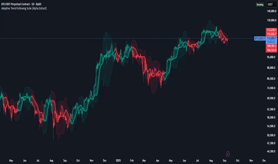
Adaptive Trend Following Suite [Alpha Extract]A sophisticated multi-filter trend analysis system that combines advanced noise reduction, adaptive moving averages, and intelligent market structure detection to deliver institutional-grade trend following signals. Utilizing cutting-edge mathematical algorithms and dynamic channel adaptation, this indicator provides crystal-clear directional guidance with real-time confidence scoring and market mode classification for professional trading execution.
🔶 Advanced Noise Reduction
Filter Eliminates market noise using sophisticated Gaussian filtering with configurable sigma values and period optimization. The system applies mathematical weight distribution across price data to ensure clean signal generation while preserving critical trend information, automatically adjusting filter strength based on volatility conditions.
advancedNoiseFilter(sourceData, filterLength, sigmaParam) =>
weightSum = 0.0
valueSum = 0.0
centerPoint = (filterLength - 1) / 2
for index = 0 to filterLength - 1
gaussianWeight = math.exp(-0.5 * math.pow((index - centerPoint) / sigmaParam, 2))
weightSum += gaussianWeight
valueSum += sourceData * gaussianWeight
valueSum / weightSum
🔶 Adaptive Moving Average Core Engine
Features revolutionary volatility-responsive averaging that automatically adjusts smoothing parameters based on real-time market conditions. The engine calculates adaptive power factors using logarithmic scaling and bandwidth optimization, ensuring optimal responsiveness during trending markets while maintaining stability during consolidation phases.
// Calculate adaptive parameters
adaptiveLength = (periodLength - 1) / 2
logFactor = math.max(math.log(math.sqrt(adaptiveLength)) / math.log(2) + 2, 0)
powerFactor = math.max(logFactor - 2, 0.5)
relativeVol = avgVolatility != 0 ? volatilityMeasure / avgVolatility : 0
adaptivePower = math.pow(relativeVol, powerFactor)
bandwidthFactor = math.sqrt(adaptiveLength) * logFactor
🔶 Intelligent Market Structure Analysis
Employs fractal dimension calculations to classify market conditions as trending or ranging with mathematical precision. The system analyzes price path complexity using normalized data arrays and geometric path length calculations, providing quantitative market mode identification with configurable threshold sensitivity.
🔶 Multi-Component Momentum Analysis
Integrates RSI and CCI oscillators with advanced Z-score normalization for statistical significance testing. Each momentum component receives independent analysis with customizable periods and significance levels, creating a robust consensus system that filters false signals while maintaining sensitivity to genuine momentum shifts.
// Z-score momentum analysis
rsiAverage = ta.sma(rsiComponent, zAnalysisPeriod)
rsiDeviation = ta.stdev(rsiComponent, zAnalysisPeriod)
rsiZScore = (rsiComponent - rsiAverage) / rsiDeviation
if math.abs(rsiZScore) > zSignificanceLevel
rsiMomentumSignal := rsiComponent > 50 ? 1 : rsiComponent < 50 ? -1 : rsiMomentumSignal
❓How It Works
🔶 Dynamic Channel Configuration
Calculates adaptive channel boundaries using three distinct methodologies: ATR-based volatility, Standard Deviation, and advanced Gaussian Deviation analysis. The system automatically adjusts channel multipliers based on market structure classification, applying tighter channels during trending conditions and wider boundaries during ranging markets for optimal signal accuracy.
dynamicChannelEngine(baselineData, channelLength, methodType) =>
switch methodType
"ATR" => ta.atr(channelLength)
"Standard Deviation" => ta.stdev(baselineData, channelLength)
"Gaussian Deviation" =>
weightArray = array.new_float()
totalWeight = 0.0
for i = 0 to channelLength - 1
gaussWeight = math.exp(-math.pow((i / channelLength) / 2, 2))
weightedVariance += math.pow(deviation, 2) * array.get(weightArray, i)
math.sqrt(weightedVariance / totalWeight)
🔶 Signal Processing Pipeline
Executes a sophisticated 10-step signal generation process including noise filtering, trend reference calculation, structure analysis, momentum component processing, channel boundary determination, trend direction assessment, consensus calculation, confidence scoring, and final signal generation with quality control validation.
🔶 Confidence Transformation System
Applies sigmoid transformation functions to raw confidence scores, providing 0-1 normalized confidence ratings with configurable threshold controls. The system uses steepness parameters and center point adjustments to fine-tune signal sensitivity while maintaining statistical robustness across different market conditions.
🔶 Enhanced Visual Presentation
Features dynamic color-coded trend lines with adaptive channel fills, enhanced candlestick visualization, and intelligent price-trend relationship mapping. The system provides real-time visual feedback through gradient fills and transparency adjustments that immediately communicate trend strength and direction changes.
🔶 Real-Time Information Dashboard
Displays critical trading metrics including market mode classification (Trending/Ranging), structure complexity values, confidence scores, and current signal status. The dashboard updates in real-time with color-coded indicators and numerical precision for instant market condition assessment.
🔶 Intelligent Alert System
Generates three distinct alert types: Bullish Signal alerts for uptrend confirmations, Bearish Signal alerts for downtrend confirmations, and Mode Change alerts for market structure transitions. Each alert includes detailed messaging and timestamp information for comprehensive trade management integration.
🔶 Performance Optimization
Utilizes efficient array management and conditional processing to maintain smooth operation across all timeframes. The system employs strategic variable caching, optimized loop structures, and intelligent update mechanisms to ensure consistent performance even during high-volatility market conditions.
This indicator delivers institutional-grade trend analysis through sophisticated mathematical modelling and multi-stage signal processing. By combining advanced noise reduction, adaptive averaging, intelligent structure analysis, and robust momentum confirmation with dynamic channel adaptation, it provides traders with unparalleled trend following precision. The comprehensive confidence scoring system and real-time market mode classification make it an essential tool for professional traders seeking consistent, high-probability trend following opportunities with mathematical certainty and visual clarity.
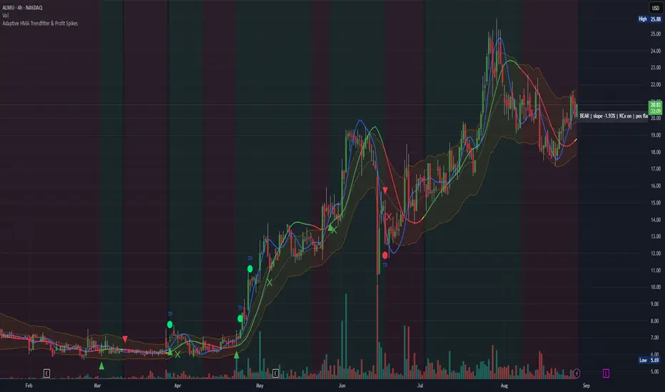
Adaptive HMA Trendfilter & Profit SpikesShort Description
Adaptive trend-following filter using Hull Moving Average (HMA) slope.
Includes optional Keltner Channel entries/exits and dynamic spike-based take-profit markers (ATR/Z-Score).
Optional Fast HMA for early entry visualization (not included in logic).
USER GUIDE:
1) Quick Overview
Trend Filter: Slow HMA defines Bull / Bear / Sideways (via slope & direction).
Entries / Exits:
Entry: Color change of the slow HMA (red→green = Long, green→red = Short), optionally filtered by the Keltner basis.
Exit: Preferably via Keltner Band (Long: Close under Upper Band; Short: Close above Lower Band).
Fallback: exit on opposite HMA color change.
Take-Profit Spikes: Marks abnormal moves (ATR, Z-Score, or both) as discretionary TP signals.
Fast HMA (optional): Purely visual for early entry opportunities; not part of the core trading logic (see §5).
2) Adding & Basic Setup
Add the indicator to your chart.
Open Settings (gear icon) and configure:
HMA: Slow HMA Length = 55, Slope Lookback = 10, Slope Threshold = 0.20%.
Keltner: KC Length = 20, Multiplier = 1.5.
Spike-TP: Mode = ATR+Z, ATR Length = 14, Z Length = 20, Cooldown = 5.
Optionally: enable Fast HMA (e.g., length = 20).
3) Input Parameters – Key Controls
Slow HMA Length: Higher = smoother, fewer but cleaner signals.
Slope Lookback: How far back HMA slope is compared against.
Slope Threshold (%): Minimum slope to avoid “Sideways” regime.
KC Length / Multiplier: Width and reactivity of Keltner Channels.
Exits via KC Bands: Toggle on/off (recommended: on).
Entries only above/below KC Basis: Helps filter out chop.
Spike Mode: Choose ATR, Z, or ATR+Z (stricter, fewer signals).
Spikes only when in position: TP markers show only when you’re in a trade.
4) Entry & Exit Logic
Entries
Long: Slow HMA turns from red → green, and (if filter enabled) Close > KC Basis.
Short: Slow HMA turns from green → red, and (if filter enabled) Close < KC Basis.
Exits
KC Exit (recommended):
Long → crossunder(close, Upper KC) closes trade.
Short → crossover(close, Lower KC).
Fallback Exit: If KC Exits are off → exit on opposite HMA color change.
Spike-TP (Discretionary)
Marks unusually large deviations from HMA.
Use for partial profits or tightening stops.
⚠️ Not auto-traded — only marker/alert.
5) Early Entry Opportunities (Fast HMA Cross – visual only)
The script can optionally display a Fast HMA (e.g., 20) alongside the Slow HMA (e.g., 55).
Bullish early hint: Fast HMA crosses above Slow HMA, or stays above, before the Slow HMA officially turns green.
Bearish early hint: opposite.
⚠️ These signals are not part of the built-in logic — they are purely discretionary:
Advantage: Earlier entries, more profit potential.
Risk: Higher chance of whipsaws.
Practical workflow (early long entry):
Fast HMA crosses above Slow HMA AND Close > KC Basis.
Enter small position with tight stop (under KC Basis or HMA swing).
Once Slow HMA confirms green → add to position or trail stop tighter.
6) Recommended Presets
Crypto (1h/2h):
HMA: 55 / 10 / 0.20–0.30%
KC: 20 / 1.5–1.8
Spikes: ATR+Z, ATR=14, Z=20, Cooldown 5
FX (1h/4h):
HMA: 55 / 8–10 / 0.10–0.25%
KC: 20 / 1.2–1.5
Indices (15m/1h):
HMA: 50–60 / 8–12 / 0.15–0.30%
KC: 20 / 1.3–1.6
Fine-tuning:
Too noisy? → Raise slope threshold or increase HMA length.
Too sluggish? → Lower slope threshold or shorten HMA length.
7) Alerts – Best Practice
Long/Short Entry – get notified when trend color switches & KC filter is valid.
Long/Short Exit – for KC exits or fallback exits.
Long/Short Spike TP – for discretionary profit-taking.
Set via TradingView: Create Alert → Select this indicator → choose condition.
8) Common Pitfalls & Tips
Too many false signals?
Raise slope threshold (more “Sideways” filtering).
Enable KC filter for entries.
Entries too late?
Use Fast HMA cross for early discretionary entries.
Or lower slope threshold slightly.
Spikes too rare/frequent?
More frequent → ATR mode or lower ATR multiplier / Z-threshold.
Rarer but stronger → ATR+Z with higher thresholds.
9) Example Playbook (Long Trade)
Regime: Slow HMA still red, Fast HMA crosses upward (early hint).
Filter: Close > KC Basis.
Early Entry: Small size, stop below KC Basis or recent swing low.
Confirmation: Slow HMA turns green → scale up or trail stop.
Management: Partial profits at Spike-TP marker; full exit at KC upper band break.
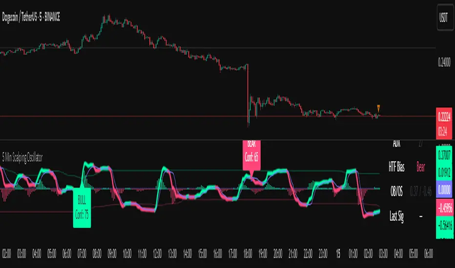
5 Min Scalping Oscillator### Overview
The 5 Min Scalping Oscillator is a custom oscillator designed to provide traders with a unified momentum signal by fusing normalized versions of the Relative Strength Index (RSI), Stochastic RSI, and Commodity Channel Index (CCI). This combination creates a more balanced view of market momentum, overbought/oversold conditions, and potential reversals, while incorporating adaptive smoothing, dynamic thresholds, and market condition filters to reduce noise and false signals. Unlike standalone oscillators, the 5 Min Scalping Oscillator adapts to trending or sideways regimes, volatility levels, and higher timeframe biases, making it particularly suited for short-term charts like 5-minute timeframes where quick, filtered signals are valuable.
### Purpose and Originality of the Fusion
Traditional oscillators like RSI measure momentum but can lag in volatile markets; Stochastic RSI adds sensitivity to RSI extremes but often generates excessive noise; and CCI identifies cyclical deviations but may overreact to minor price swings. The 5 Min Scalping Oscillator addresses these limitations by weighting and blending their normalized outputs (RSI at 45%, Stochastic RSI at 35%, and CCI at 20%) into a single raw oscillator value. This weighted fusion creates a hybrid signal that balances lag reduction with noise filtering, resulting in a more robust indicator for identifying reversal opportunities.
The originality lies in extending this fusion with:
- **Adaptive Smoothing via KAMA (Kaufman's Adaptive Moving Average):** Adjusts responsiveness based on market efficiency, speeding up in trends and slowing in ranges—unlike fixed EMAs, this helps preserve signal integrity without over-smoothing.
- **Dynamic Overbought/Oversold Thresholds:** Calculated using rolling percentiles over a user-defined lookback (default 200+ periods), these levels adapt to recent oscillator behavior rather than relying on static values like 70/30, making the indicator more responsive to asset-specific volatility.
- **Multi-Factor Filters:** Integrates ADX for trend detection, ATR percentiles for volatility confirmation, and optional higher timeframe RSI bias to ensure signals align with broader market context. This layered approach reduces false positives (e.g., ignoring low-volatility crossovers) and adds a confidence score based on filter alignment, which is not typically found in simple mashups.
This design justifies the combination: it's not a mere overlay of indicators but a purposeful integration that enhances usefulness by providing context-aware signals, helping traders avoid common pitfalls like trading against the trend or in low-volatility chop. The result is an original tool that performs better in diverse conditions, especially on 5-minute charts for intraday trading, where rapid adaptations are key.
### How It Works
The 5 Min Scalping Oscillator processes price data through these steps:
1. **Normalization and Fusion:**
- RSI (default length 10) is normalized to a -1 to +1 scale using a tanh transformation for bounded output.
- Stochastic RSI (default length 14) is derived from RSI highs/lows and scaled similarly.
- CCI (default length 14) is tanh-normalized to align with the others.
- These are weighted and summed into a raw value, emphasizing RSI for core momentum while using Stochastic RSI for edge sensitivity and CCI for cycle detection.
2. **Smoothing and Signal Line:**
- The raw value is smoothed (default KAMA with fast/slow periods 2/30 and efficiency length 10) to reduce whipsaws.
- A shorter signal line (half the smoothing length) is added for crossover detections.
3. **Filters and Enhancements:**
- **Trend Regime:** ADX (default length 14, threshold 20) classifies markets as trending (ADX > threshold) or sideways, allowing signals in both but prioritizing alignment.
- **Volatility Check:** ATR (default length 14) percentile (default 85%) ensures signals only trigger in above-average volatility, filtering out flat markets.
- **Higher Timeframe Bias:** Optional RSI (default length 14 on 60-minute timeframe) provides bull/neutral/bear bias (above 55, 45-55, below 45), requiring signal alignment (e.g., bullish signals only if bias is neutral or bull).
- **Dynamic Levels:** Percentiles (default OB 85%, OS 15%) over recent oscillator values set adaptive overbought/oversold lines.
4. **Signal Generation:**
- Bullish (B) signals on upward crossovers of the smoothed line over the signal line, filtered by conditions.
- Bearish (S) signals on downward crossunders.
- Each signal includes a confidence score (0-100) based on factors like trend alignment (25 points), volatility (15 points), and bias (20 points if strong, 10 if neutral).
The output includes a glowing oscillator line, histogram for divergence spotting, dynamic levels, shapes/labels for signals, and a dashboard table summarizing regime, ADX, bias, levels, and last signal.
### How to Use It
This indicator is easy to apply and interpret, even for beginners:
- **Adding to Chart:** Apply the 5 Min Scalping Oscillator to a clean chart (no other indicators unless explained). It's non-overlay, so it appears in a separate pane. For 5-minute timeframes, keep defaults or tweak lengths shorter for faster response (e.g., RSI 8-12).
- **Interpreting Signals:**
- Look for green upward triangles labeled "B" (bullish) at the bottom for potential entry opportunities in uptrends or reversals.
- Red downward triangles labeled "S" (bearish) at the top signal potential exits or shorts.
- Higher confidence scores (e.g., 70+) indicate stronger alignment—use these for priority trades.
- Watch the histogram for divergences (e.g., price higher highs but histogram lower highs suggest weakening momentum).
- Dynamic OB (green line) and OS (red line) help gauge extremes; signals near these are more reliable.
- **Dashboard:** At the bottom-right, it shows real-time info like "Trending" or "Sideways" regime, ADX value, HTF bias (Bull/Neutral/Bear), OB/OS levels, and last signal—use this for quick context.
- **Customization:** Adjust inputs via the settings panel:
- Toggle KAMA for adaptive vs. EMA smoothing.
- Set HTF to "60" for 1-hour bias on 5-min charts.
- Increase ADX threshold to 25 for stricter trend filtering.
- **Best Practices:** Combine with price action (e.g., support/resistance) or volume for confirmation. On 5-min charts, pair with a 1-hour HTF for intraday scalping. Always use stop-losses and risk no more than 1-2% per trade.
### Default Settings Explanation
Defaults are optimized for 5-minute charts on volatile assets like stocks or forex:
- RSI/Stoch/CCI lengths (10/14/14): Shorter for quick momentum capture.
- Signal smoothing (5): Responsive without excessive lag.
- ADX threshold (20): Balances trend detection.
- ATR percentile (0.85): Filters ~15% of low-vol signals.
- HTF RSI (14 on 60-min): Aligns with hourly trends.
- Percentiles (OB 85%, OS 15%): Adaptive to recent data.
If changing, test on historical data to ensure fit—e.g., longer lengths for less noisy assets.
### Disclaimer
The 5 Min Scalping Oscillator is an educational tool to visualize momentum and does not guarantee profits or predict future performance. All signals are based on historical calculations and should not be used as standalone trading advice. Past results are not indicative of future outcomes. Traders must conduct their own analysis, use proper risk management, and consider market conditions. No claims are made about accuracy, reliability, or performance.
Adaptive Market Profile – Auto Detect & Dynamic Activity ZonesAdaptive Market Profile is an advanced indicator that automatically detects and displays the most relevant trend channel and market profile for any asset and timeframe. Unlike standard regression channel tools, this script uses a fully adaptive approach to identify the optimal period, providing you with the channel that best fits the current market dynamics. The calculation is based on maximizing the statistical significance of the trend using Pearson’s R coefficient, ensuring that the most relevant trend is always selected.
Within the selected channel, the indicator generates a dynamic market profile, breaking the price range into configurable zones and displaying the most active areas based on volume or the number of touches. This allows you to instantly identify high-activity price levels and potential support/resistance zones. The “most active lines” are plotted in real-time and always stay parallel to the channel, dynamically adapting to market structure.
Key features:
- Automatic detection of the optimal regression period: The script scans a wide range of lengths and selects the channel that statistically represents the strongest trend.
- Dynamic market profile: Visualizes the distribution of volume or price touches inside the trend channel, with customizable section count.
- Most active zones: Highlights the most traded or touched price levels as dynamic, parallel lines for precise support/resistance reading.
- Manual override: Optionally, users can select their own channel period for full control.
- Supports both linear and logarithmic charts: Simple toggle to match your chart scaling.
Use cases:
- Trend following and channel trading strategies.
- Quick identification of dynamic support/resistance and liquidity zones.
- Objective selection of the most statistically significant trend channel, without manual guesswork.
- Suitable for all assets and timeframes (crypto, stocks, forex, futures).
Originality:
This script goes beyond basic regression channels by integrating dynamic profile analysis and fully adaptive period detection, offering a comprehensive tool for modern technical analysts. The combination of trend detection, market profile, and activity zone mapping is unique and not available in TradingView built-ins.
Instructions:
Add Adaptive Market Profile to your chart. By default, the script automatically detects the optimal channel period and displays the corresponding regression channel with dynamic profile and activity zones. If you prefer manual control, disable “Auto trend channel period” and set your preferred period. Adjust profile settings as needed for your asset and timeframe.
For questions, suggestions, or further customization, contact Julien Eche (@Julien_Eche) directly on TradingView.

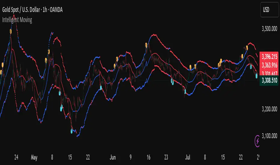
Intelligent Moving📘 Intelligent Moving – Adaptive Neural Trend Engine
Intelligent Moving is an invite-only, closed-source indicator that dynamically adjusts itself to evolving market conditions using a built-in neural optimizer. It combines a custom adaptive Moving Average, ATR-based deviation bands, and a fully internal virtual trade simulator to deliver smart trend signals and automatic parameter tuning — all without repainting or manual intervention.
This script is built entirely from original code and does not use any open-source components or built-in TradingView indicators.
🧠 Core Logic and Visual Structure
The indicator plots:
- A central moving average (optimized dynamically),
- Upper and lower deviation bands based on ATR × adaptive coefficients,
- Buy (aqua) and Sell (orange) arrows on reversion signals,
- Color-coded trend zones based on price vs. moving average.
All three bands change color in real time depending on the price’s position relative to the MA, clearly showing uptrends (e.g. blue) and downtrends (e.g. red).
📈 Signal Logic: Reversion from Extremes
- Buy Signal: After price closes below the lower deviation band, it then closes back above it.
- Sell Signal: After price closes above the upper deviation band, it then closes back below it.
These signals are not based on crossovers, oscillators, or lagging logic — they are pure structure-based reversion entries, designed to detect exhaustion and reversal zones.
🤖 Built-In Neural Optimizer (Perceptron Engine)
At the heart of Intelligent Moving lies a self-training engine that uses simulated (virtual) positions to test multiple configurations and pick the best one. Here’s how it works:
🔄 Virtual Trade Simulation
At regular intervals (user-defined), the script:
- Simulates virtual buy/sell positions based on its signal logic.
- Applies virtual Stop-Loss (just beyond the signal zone) and virtual Take-Profit (when price crosses back over the MA).
- Calculates simulated profit for each combination of:
- - MA periods,
- - Upper/lower ATR multipliers.
🧠 Neural Training Process
- A perceptron-like engine evaluates the simulated results.
- It selects the best-performing configuration and applies it to live plotting.
- You can choose whether optimization uses a base value or the last best result from the previous training pass.
This process runs forward-only and never overwrites history or uses future data. It's completely transparent and non-repainting.
⚙️ Customization and Parameters
Users can control:
- MA period range, step, and training type (base vs last best)
- Deviation multiplier ranges and step
- Training depth (number of bars in history)
- Training interval (how often to retrain)
- Spread simulation, alert options, and all visual settings
💡 What Makes It Unique
- ✅ Self-optimization with virtual trades and perceptron logic
- ✅ Adaptive deviation bands based on ATR (not standard deviation)
- ✅ No built-in indicators, no repaints, no curve-fitting
- ✅ Clear trend zones and reversal signals
- ✅ Optimized for live use and consistent behavior across assets
Unlike typical moving average tools, Intelligent Moving thinks, adapts, and reacts — turning a standard concept into a living, learning trend engine.
📊 Use Cases
- Trend detection with adaptive coloring
- Reversion trading from volatility extremes
- Dynamic strategy building with minimal manual input
- Alerts for automated or discretionary traders
🔒 Invite-Only Notice
This script is invite-only and closed-source.
The optimization logic, trade simulation system, and perceptron engine were developed from scratch, specifically for this indicator. No built-in functions (e.g. MA, BB, RSI) or public scripts were used or copied.
All decisions and calculations are based on current and past price only — no repainting, retrofitting, or future leakage.
⚠️ Disclaimer
This indicator is for educational and analytical use only.
It does not predict future prices or guarantee profits. Always use appropriate risk management and test thoroughly before live trading.
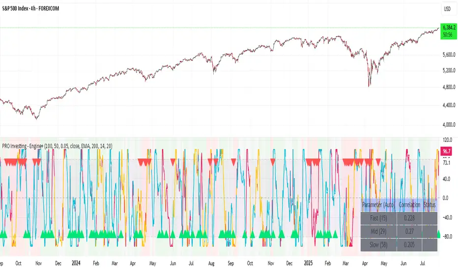
PRO Investing - Apex EnginePRO Investing - Apex Engine
1. Core Concept: Why Does This Indicator Exist?
Traditional momentum oscillators like RSI or Stochastic use a fixed "lookback period" (e.g., 14). This creates a fundamental problem: a 14-period setting that works well in a fast, trending market will generate constant false signals in a slow, choppy market, and vice-versa. The market's character is dynamic, but most tools are static.
The Apex Engine was built to solve this problem. Its primary innovation is a self-optimizing core that continuously adapts to changing market conditions. Instead of relying on one fixed setting, it actively tests three different momentum profiles (Fast, Mid, and Slow) in real-time and selects the one that is most synchronized with the current price action.
This is not just a random combination of indicators; it's a deliberate synthesis designed to create a more robust momentum tool. It combines:
Volatility analysis (ATR) to generate adaptive lookback periods.
Momentum measurement (ROC) to gauge the speed of price changes.
Statistical analysis (Correlation) to validate which momentum measurement is most effective right now.
Classic trend filters (Moving Average, ADX) to ensure signals are only taken in favorable market conditions.
The result is an oscillator that aims to be more responsive in volatile trends and more stable in quiet periods, providing a more intelligent and adaptive signal.
2. How It Works: The Engine's Three-Stage Process
To be transparent, it's important to understand the step-by-step logic the indicator follows on every bar. It's a process of Adapt -> Validate -> Signal.
Stage 1: Adapt (Dynamic Length Calculation)
The engine first measures market volatility using the Average True Range (ATR) relative to its own long-term average. This creates a volatility_factor. In high-volatility environments, this factor causes the base calculation lengths to shorten. In low-volatility, they lengthen. This produces three potential Rate of Change (ROC) lengths: dynamic_fast_len, dynamic_mid_len, and dynamic_slow_len.
Stage 2: Validate (Self-Optimizing Mode Selection)
This is the core of the engine. It calculates the ROC for all three dynamic lengths. To determine which is best, it uses the ta.correlation() function to measure how well each ROC's movement has correlated with the actual bar-to-bar price changes over the "Optimization Lookback" period. The ROC length with the highest correlation score is chosen as the most effective profile for the current moment. This "active" mode is reflected in the oscillator's color and the dashboard.
Stage 3: Signal (Normalized Velocity Oscillator)
The winning ROC series is then normalized into a consistent oscillator (the Velocity line) that ranges from -100 (extreme oversold) to +100 (extreme overbought). This ensures signals are comparable across any asset or timeframe. Signals are only generated when this Velocity line crosses its signal line and the trend filters (explained below) give a green light.
3. How to Use the Indicator: A Practical Guide
Reading the Visuals:
Velocity Line (Blue/Yellow/Pink): The main oscillator line. Its color indicates which mode is active (Fast, Mid, or Slow).
Signal Line (White): A moving average of the Velocity line. Crossovers generate potential signals.
Buy/Sell Triangles (▲ / ▼): These are your primary entry signals. They are intentionally strict and only appear when momentum, trend, and price action align.
Background Color (Green/Red/Gray): This is your trend context.
Green: Bullish trend confirmed (e.g., price above a rising 200 EMA and ADX > 20). Only Buy signals (▲) can appear.
Red: Bearish trend confirmed. Only Sell signals (▼) can appear.
Gray: No clear trend. The market is likely choppy or consolidating. No signals will appear; it is best to stay out.
Trading Strategy Example:
Wait for a colored background. A green or red background indicates the market is in a tradable trend.
Look for a signal. For a green background, wait for a lime Buy triangle (▲) to appear.
Confirm the trade. Before entering, confirm the signal aligns with your own analysis (e.g., support/resistance levels, chart patterns).
Manage the trade. Set a stop-loss according to your risk management rules. An exit can be considered on a fixed target, a trailing stop, or when an opposing signal appears.
4. Settings and Customization
This script is open-source, and its settings are transparent. You are encouraged to understand them.
Synaptic Engine Group:
Volatility Period: The master control for the adaptive engine. Higher values are slower and more stable.
Optimization Lookback: How many bars to use for the correlation check.
Switch Sensitivity: A buffer to prevent frantic switching between modes.
Advanced Configuration & Filters Group:
Price Source: The data source for momentum calculation (default close).
Trend Filter MA Type & Length: Define your long-term trend.
Filter by MA Slope: A key feature. If ON, allows for "buy the dip" entries below a rising MA. If OFF, it's stricter, requiring price to be above the MA.
ADX Length & Threshold: Filters out non-trending, choppy markets. Signals will not fire if the ADX is below this threshold.
5. Important Disclaimer
This indicator is a decision-support tool for discretionary traders, not an automated trading system or financial advice. Past performance is not indicative of future results. All trading involves substantial risk. You should always use proper risk management, including setting stop-losses, and never risk more than you are prepared to lose. The signals generated by this script should be used as one component of a broader trading plan.
RSI Mansfield +RSI Mansfield+ – Adaptive Relative Strength Indicator with Divergences
Overview
RSI Mansfield+ is an advanced relative strength indicator that compares your instrument’s performance against a configurable benchmark index or asset (e.g., Bitcoin Dominance, S&P 500). It combines Mansfield normalization, adaptive smoothing techniques, and automatic detection of bullish and bearish divergences (regular and hidden), delivering a comprehensive tool for assessing relative strength across any market and timeframe.
Originality and Motivation
Unlike traditional relative strength scripts, this indicator introduces several distinctive improvements:
Mansfield Normalization: Scales the ratio between the asset and the benchmark relative to its moving average, transforming it into a normalized oscillator that fluctuates around zero, making it easier to spot outperformance or underperformance.
Adaptive Smoothing: Automatically selects whether to use EMA or SMA based on the market type (crypto or stocks) and timeframe (intraday, daily, weekly, monthly), avoiding manual configuration and providing more robust results under varying volatility conditions.
Divergence Detection: Identifies four types of divergences in the Mansfield oscillator to help anticipate potential reversal points or trend confirmations.
Multi-Market Support: Offers benchmark selection among major crypto and global stock indices from a single input.
These enhancements make RSI Mansfield+ more practical and powerful than conventional relative strength scripts with static benchmarks or without divergence capabilities.
Core Concepts
Relative Strength (RS): Compares price evolution between your asset and the selected benchmark.
Mansfield Normalization: Measures how much the RS deviates from its historical moving average, expressed as a scaled oscillator.
Divergences: Detects regular and hidden bullish or bearish divergences within the Mansfield oscillator.
Timeframe Adaptation: Dynamically adjusts moving average lengths based on timeframe and market type.
How It Works
Benchmark Selection
Choose among over 10 indices or market domains (BTC Dominance, ETH Dominance, S&P 500, European indices, etc.).
Ratio Calculation
Computes the price-to-benchmark ratio and smooths it with the adaptive moving average.
Normalization and Scaling
Transforms deviations into a Mansfield oscillator centered around zero.
Dynamic Coloring
Green indicates relative outperformance, red signals underperformance.
Divergence Detection
Automatically identifies bullish and bearish (regular and hidden) divergences by comparing oscillator pivots against price pivots.
Baseline Reference
A clear zero line helps interpret relative strength trends.
Usage Guidelines
Benchmark Comparison
Ideal for traders analyzing whether an asset is outperforming or lagging its sector or market.
Divergence Analysis
Helps detect potential reversal or continuation signals in relative strength.
Multi-Timeframe Compatibility
Can be applied to intraday, daily, weekly, or monthly charts.
Interpretation
Oscillator >0 and green: outperforming the benchmark.
Oscillator <0 and red: underperforming.
Bullish divergences: potential relative strength reversal to the upside.
Bearish divergences: possible loss of momentum or reversal to the downside.
Credits
The concept of Mansfield Relative Strength is based on Stan Weinstein’s original work on relative performance analysis. This script was built entirely from scratch in TradingView Pine Script v6, incorporating original logic for adaptive smoothing, normalized scaling, and divergence detection, without reusing any external open-source code.

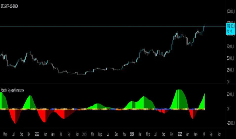
Adaptive Squeeze Momentum +Adaptive Squeeze Momentum+ (Auto-Timeframe Version)
Overview
Adaptive Squeeze Momentum+ is an enhanced volatility and momentum indicator designed to identify compression and expansion phases in price action. It is inspired by the classic Squeeze Momentum Indicator by LazyBear but introduces automatic parameter adaptation to any timeframe, making it simpler to use across different markets without manual configuration.
Concepts and Methodology
The script combines Bollinger Bands (BB) and Keltner Channels (KC) to detect periods when volatility contracts (squeeze) or expands (release).
A squeeze occurs when BB are inside KC, suggesting low volatility and potential breakout scenarios.
A squeeze release is detected when BB expand outside KC.
Momentum is derived using a linear regression applied to the difference between price and a midrange reference level.
Original Improvements
Compared to the original Squeeze Momentum Indicator, this version offers several enhancements:
Automatic Adaptation: BB and KC lengths and multipliers are dynamically adjusted based on the chart’s timeframe (from 1 minute up to 1 month), removing the need for manual tuning.
Simplified Visualization: A clean, minimalist histogram and clear squeeze state cross markers allow for faster interpretation.
Flexible Application: Designed to work consistently on intraday, daily, and higher timeframes across crypto, forex, stocks, and indices.
Features
Dynamic Squeeze Detection:
Gray Cross: Neutral (no squeeze detected)
Blue Cross: Active squeeze
Yellow Cross: Squeeze released
Momentum Histogram:
Positive/negative momentum shown with slope-based coloring.
Timeframe-Aware Parameters:
Automatically sets optimal BB/KC configurations.
Usage
Watch for blue crosses indicating an active squeeze phase that may precede a directional move.
Use the histogram color and slope to gauge momentum strength and direction.
Combine squeeze release signals with momentum confirmation for potential entries or exits.
Credits and Licensing
This script was inspired by LazyBear’s OLD “Squeeze Momentum Indicator” (). The implementation here significantly expands upon the original by introducing auto-adaptive parameters, restructured logic, and a new visualization approach. Published under the Mozilla Public License 2.0.
Disclaimer
This indicator is for educational purposes only and does not constitute financial advice. Use at your own risk.
Active PMI Support/Resistance Levels [EdgeTerminal]The PMI Support & Resistance indicator revolutionizes traditional technical analysis by using Pointwise Mutual Information (PMI) - a statistical measure from information theory - to objectively identify support and resistance levels. Unlike conventional methods that rely on visual pattern recognition, this indicator provides mathematically rigorous, quantifiable evidence of price levels where significant market activity occurs.
- The Mathematical Foundation: Pointwise Mutual Information
Pointwise Mutual Information measures how much more likely two events are to occur together compared to if they were statistically independent. In our context:
Event A: Volume spikes occurring (high trading activity)
Event B: Price being at specific levels
The PMI formula calculates: PMI = log(P(A,B) / (P(A) × P(B)))
Where:
P(A,B) = Probability of volume spikes occurring at specific price levels
P(A) = Probability of volume spikes occurring anywhere
P(B) = Probability of price being at specific levels
High PMI scores indicate that volume spikes and certain price levels co-occur much more frequently than random chance would predict, revealing genuine support and resistance zones.
- Why PMI Outperforms Traditional Methods
Subjective interpretation: What one trader sees as significant, another might ignore
Confirmation bias: Tendency to see patterns that confirm existing beliefs
Inconsistent criteria: No standardized definition of "significant" volume or price action
Static analysis: Doesn't adapt to changing market conditions
No strength measurement: Can't quantify how "strong" a level truly is
PMI Advantages:
✅ Objective & Quantifiable: Mathematical proof of significance, not visual guesswork
✅ Statistical Rigor: Levels backed by information theory and probability
✅ Strength Scoring: PMI scores rank levels by statistical significance
✅ Adaptive: Automatically adjusts to different market volatility regimes
✅ Eliminates Bias: Computer-calculated, removing human interpretation errors
✅ Market Structure Aware: Reveals the underlying order flow concentrations
- How It Works
Data Processing Pipeline:
Volume Analysis: Identifies volume spikes using configurable thresholds
Price Binning: Divides price range into discrete levels for analysis
Co-occurrence Calculation: Measures how often volume spikes happen at each price level
PMI Computation: Calculates statistical significance for each price level
Level Filtering: Shows only levels exceeding minimum PMI thresholds
Dynamic Updates: Refreshes levels periodically while maintaining historical traces
Visual System:
Current Levels: Bright, thick lines with PMI scores - your actionable levels
Historical Traces: Faded previous levels showing market structure evolution
Strength Tiers: Line styles indicate PMI strength (solid/dashed/dotted)
Color Coding: Green for support, red for resistance
Info Table: Real-time display of strongest levels with scores
- Indicator Settings:
Core Parameters
Lookback Period (Default: 200)
Lower (50-100): More responsive to recent price action, catches short-term levels
Higher (300-500): Focuses on major historical levels, more stable but less responsive
Best for: Day trading (100-150), Swing trading (200-300), Position trading (400-500)
Volume Spike Threshold (Default: 1.5)
Lower (1.2-1.4): More sensitive, catches smaller volume increases, more levels detected
Higher (2.0-3.0): Only major volume surges count, fewer but stronger signals
Market dependent: High-volume stocks may need higher thresholds (2.0+), low-volume stocks lower (1.2-1.3)
Price Bins (Default: 50)
Lower (20-30): Broader price zones, less precise but captures wider areas
Higher (70-100): More granular levels, precise but may be overly specific
Volatility dependent: High volatility assets benefit from more bins (70+)
Minimum PMI Score (Default: 0.5)
Lower (0.2-0.4): Shows more levels including weaker ones, comprehensive view
Higher (1.0-2.0): Only statistically strong levels, cleaner chart
Progressive filtering: Start with 0.5, increase if too cluttered
Max Levels to Show (Default: 8)
Fewer (3-5): Clean chart focusing on strongest levels only
More (10-15): Comprehensive view but may clutter chart
Strategy dependent: Scalpers prefer fewer (3-5), swing traders more (8-12)
Historical Tracking Settings
Update Frequency (Default: 20 bars)
Lower (5-10): More frequent updates, captures rapid market changes
Higher (50-100): Less frequent updates, focuses on major structural shifts
Timeframe scaling: 1-minute charts need lower frequency (5-10), daily charts higher (50+)
Show Historical Levels (Default: True)
Enables the "breadcrumb trail" effect showing evolution of support/resistance
Disable for cleaner charts focusing only on current levels
Max Historical Marks (Default: 50)
Lower (20-30): Less memory usage, shorter history
Higher (100-200): Longer historical context but more resource intensive
Fade Strength (Default: 0.8)
Lower (0.5-0.6): Historical levels more visible
Higher (0.9-0.95): Historical levels very subtle
Visual Settings
Support/Resistance Colors: Choose colors that contrast well with your chart theme Line Width: Thicker lines (3-4) for better visibility on busy charts Show PMI Scores: Toggle labels showing statistical strength Label Size: Adjust based on screen resolution and chart zoom level
- Most Effective Usage Strategies
For Day Trading:
Setup: Lookback 100-150, Volume Threshold 1.8-2.2, Update Frequency 10-15
Use PMI levels as bounce/rejection points for scalp entries
Higher PMI scores (>1.5) offer better probability setups
Watch for volume spike confirmations at levels
For Swing Trading:
Setup: Lookback 200-300, Volume Threshold 1.5-2.0, Update Frequency 20-30
Enter on pullbacks to high PMI support levels
Target next resistance level with PMI score >1.0
Hold through minor levels, exit at major PMI levels
For Position Trading:
Setup: Lookback 400-500, Volume Threshold 2.0+, Update Frequency 50+
Focus on PMI scores >2.0 for major structural levels
Use for portfolio entry/exit decisions
Combine with fundamental analysis for timing
- Trading Applications:
Entry Strategies:
PMI Bounce Trades
Price approaches high PMI support level (>1.0)
Wait for volume spike confirmation (orange triangles)
Enter long on bullish price action at the level
Stop loss just below the PMI level
Target: Next PMI resistance level
PMI Breakout Trades
Price consolidates near high PMI level
Volume increases (watch for orange triangles)
Enter on decisive break with volume
Previous resistance becomes new support
Target: Next major PMI level
PMI Rejection Trades
Price approaches PMI resistance with momentum
Watch for rejection signals and volume spikes
Enter short on failure to break through
Stop above the PMI level
Target: Next PMI support level
Risk Management:
Stop Loss Placement
Place stops 0.1-0.5% beyond PMI levels (adjust for volatility)
Higher PMI scores warrant tighter stops
Use ATR-based stops for volatile assets
Position Sizing
Larger positions at PMI levels >2.0 (highest conviction)
Smaller positions at PMI levels 0.5-1.0 (lower conviction)
Scale out at multiple PMI targets
- Key Warning Signs & What to Watch For
Red Flags:
🚨 Very Low PMI Scores (<0.3): Weak statistical significance, avoid trading
🚨 No Volume Confirmation: PMI level without recent volume spikes may be stale
🚨 Overcrowded Levels: Too many levels close together suggests poor parameter tuning
🚨 Outdated Levels: Historical traces are reference only, not tradeable
Optimization Tips:
✅ Regular Recalibration: Adjust parameters monthly based on market regime changes
✅ Volume Context: Always check for recent volume activity at PMI levels
✅ Multiple Timeframes: Confirm PMI levels across different timeframes
✅ Market Conditions: Higher thresholds during high volatility periods
Interpreting PMI Scores
PMI Score Ranges:
0.5-1.0: Moderate statistical significance, proceed with caution
1.0-1.5: Good significance, reliable for most trading strategies
1.5-2.0: Strong significance, high-confidence trade setups
2.0+: Very strong significance, institutional-grade levels
Historical Context: The historical trace system shows how support and resistance evolve over time. When current levels align with multiple historical traces, it indicates persistent market memory at those prices, significantly increasing the level's reliability.
Adaptive Causal Wavelet Trend FilterThe Adaptive Causal Wavelet Trend Filter is a technical indicator implementing causal approximations of wavelet transform properties for better trend detection with adaptive volatility response.
The Adaptive Causal Wavelet Trend Filter (ACWTF) applies mathematical principles derived from wavelet analysis to financial time series, providing robust trend identification with minimal lag. Unlike conventional moving averages, it preserves significant price movements while filtering market noise through signal processing that i describe below.
I was inspired to build this indicator after reading " Wavelet-Based Trend Identification in Financial Time Series " by In, F., & Kim, S. 2013 and reading about Mexican Hat wavelet filters.
The ACWTF maintains optimal performance across varying market regimes without requiring parameter adjustments by adapting filter characteristics to current volatility conditions.
Mathematical Foundation
Inspired by the Mexican Hat wavelet (Ricker wavelet), this indicator implements causal approximations of wavelet filters optimized for real-time financial analysis. The multi-resolution approach identifies features at different scales and the adaptive component dynamically adjusts filtering characteristics based on local volatility measurements.
Key mathematical properties include:
Non-linear frequency response adaptation
Edge-preserving signal extraction
Scale-space analysis through dual filter implementation
Volatility-dependent coefficient adjustment, which I love
Filter Methods
Adaptive: Implements a volatility-weighted combination of multiple filter types to optimize the time-frequency resolution trade-off
Hull: Provides a causal approximation of wavelet edge detection properties with forward-projection characteristics
VWMA: Incorporates volume information into the filtering process for enhanced signal detection
EMA Cascade: Creates a multi-pole filter structure that approximates certain wavelet scaling properties
Suggestion: try all as they will provide slightly different signals. Try also different time-frames.
Practical Applications
Trend Direction Identification: Clear visual trend direction with reduced noise and lag
Regime Change Detection: Early identification of significant trend reversals
Market Condition Analysis: Integrated volatility metrics provide context for current market behavior
Multi-timeframe Confirmation: Alignment between primary and secondary filters offers additional confirmation
Entry/Exit Timing: Filter crossovers and trend changes provide potential trading signals
The comprehensive information panel provides:
Current filter method and trend state
Trend alignment between timeframes
Real-time volatility assessment
Price position relative to filter
Overall trading bias based on multiple factors
Implementation Notes
Log returns option provides improved statistical properties for financial time series
Primary and secondary filter lengths can be adjusted to optimize for specific instruments and timeframes
The indicator performs particularly well during trend transitions and regime changes
The indicator reduces the need for using additional indicators to check trend reversion

Adaptive Quadratic Kernel EnvelopeThis study draws a fair-value curve from a quadratic-weighted (Nadaraya-Watson) regression. Alpha sets how sharply weights decay inside the look-back window, so you trade lag against smoothness with one slider. Band half-width is ATRslow times a bounded fast/slow ATR ratio, giving an instant response to regime shifts without overshooting on spikes. Work in log space when an instrument grows exponentially, equal percentage moves then map to equal vertical steps. NearBase and FarBase define a progression of adaptive thresholds, useful for sizing exits or calibrating mean-reversion logic. Non-repaint mode keeps one-bar delay for clean back-tests, predictive mode shows the zero-lag curve for live decisions.
Key points
- Quadratic weights cut phase error versus Gaussian or SMA-based envelopes.
- Dual-ATR scaling updates width on the next bar, no residual lag.
- Log option preserves envelope symmetry across multi-decade data.
- Alpha provides direct control of curvature versus noise.
- Built-in alerts trigger on the first adaptive threshold, ready for automation.
Typical uses
Trend bias from the slope of the curve.
Entry timing when price pierces an inner threshold and momentum stalls.
Breakout confirmation when closes hold beyond outer thresholds while volatility expands.
Stops and targets anchored to chosen thresholds, automatically matching current noise.

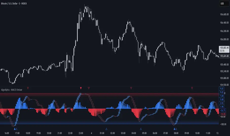
Adaptive MACD Deluxe [AlgoAlpha]OVERVIEW
This script is an advanced rework of the classic MACD indicator, designed to be more adaptive, visually informative, and customizable. It enhances the original MACD formula using a dynamic feedback loop and a correlation-based weighting system that adjusts in real-time based on how deterministic recent price action is. The signal line is flexible, offering several smoothing types including Heiken Ashi, while the histogram is color-coded with gradients to help users visually identify momentum shifts. It also includes optional normalization by volatility, allowing MACD values to be interpreted as relative percentage moves, making the indicator more consistent across different assets and timeframes.
CONCEPTS
This version of MACD introduces a deterministic weight based on R-squared correlation with time, which modulates how fast or slow the MACD adapts to price changes. Higher correlation means smoother, slower MACD responses, and low correlation leads to quicker reaction. The momentum calculation blends traditional EMA math with feedback and damping components to create a smoother, less noisy series. Heiken Ashi is optionally used for signal smoothing to better visualize short-term trend bias. When normalization is enabled, the MACD is scaled by an EMA of the high-low range, converting it into a bounded, volatility-relative indicator. This makes extreme readings more meaningful across markets.
FEATURES
The script offers six distinct options for signal line smoothing: EMA, SMA, SMMA (RMA), WMA, VWMA, and a custom Heiken Ashi mode based on the MACD series. Each option provides a different response speed and smoothing behavior, allowing traders to match the indicator’s behavior to their strategy—whether it's faster reaction or reduced noise.
Normalization is another key feature. When enabled, MACD values are scaled by a volatility proxy, converting the indicator into a relative percentage. This helps standardize the MACD across different assets and timeframes, making overbought and oversold readings more consistent and easier to interpret.
Threshold zones can be customized using upper and lower boundaries, with inner zones for early warnings. These zones are highlighted on the chart with subtle background fills and directional arrows when MACD enters or exits key levels. This makes it easier to spot strong or weak reversals at a glance.
Lastly, the script includes multiple built-in alerts. Users can set alerts for MACD crossovers, histogram flips above or below zero, and MACD entries into strong or weak reversal zones. This allows for hands-free monitoring and quick decision-making without staring at the chart.
USAGE
To use this script, choose your preferred signal smoothing type, enable normalization if you want MACD values relative to volatility, and adjust the threshold zones to fit your asset or timeframe. Use the colored histogram to detect changes in momentum strength—brighter colors indicate rising strength, while faded colors imply weakening. Heiken Ashi mode smooths out noise and provides clearer signals, especially useful in choppy conditions. Use alert conditions for crossover and reversal detection, or monitor the arrow markers for entries into potential exhaustion zones. This setup works well for trend following, momentum trading, and reversal spotting across all market types.
CNN Statistical Trading System [PhenLabs]📌 DESCRIPTION
An advanced pattern recognition system utilizing Convolutional Neural Network (CNN) principles to identify statistically significant market patterns and generate high-probability trading signals.
CNN Statistical Trading System transforms traditional technical analysis by applying machine learning concepts directly to price action. Through six specialized convolution kernels, it detects momentum shifts, reversal patterns, consolidation phases, and breakout setups simultaneously. The system combines these pattern detections using adaptive weighting based on market volatility and trend strength, creating a sophisticated composite score that provides both directional bias and signal confidence on a normalized -1 to +1 scale.
🚀 CONCEPTS
• Built on Convolutional Neural Network pattern recognition methodology adapted for financial markets
• Six specialized kernels detect distinct price patterns: upward/downward momentum, peak/trough formations, consolidation, and breakout setups
• Activation functions create non-linear responses with tanh-like behavior, mimicking neural network layers
• Adaptive weighting system adjusts pattern importance based on current market regime (volatility < 2% and trend strength)
• Multi-confirmation signals require CNN threshold breach (±0.65), RSI boundaries, and volume confirmation above 120% of 20-period average
🔧 FEATURES
Six-Kernel Pattern Detection:
Simultaneous analysis of upward momentum, downward momentum, peak/resistance, trough/support, consolidation, and breakout patterns using mathematically optimized convolution kernels.
Adaptive Neural Architecture:
Dynamic weight adjustment based on market volatility (ATR/Price) and trend strength (EMA differential), ensuring optimal performance across different market conditions.
Professional Visual Themes:
Four sophisticated color palettes (Professional, Ocean, Sunset, Monochrome) with cohesive design language. Default Monochrome theme provides clean, distraction-free analysis.
Confidence Band System:
Upper and lower confidence zones at 150% of threshold values (±0.975) help identify high-probability signal areas and potential exhaustion zones.
Real-Time Information Panel:
Live display of CNN score, market state with emoji indicators, net momentum, confidence percentage, and RSI confirmation with dynamic color coding based on signal strength.
Individual Feature Analysis:
Optional display of all six kernel outputs with distinct visual styles (step lines, circles, crosses, area fills) for advanced pattern component analysis.
User Guide
• Monitor CNN Score crossing above +0.65 for long signals or below -0.65 for short signals with volume confirmation
• Use confidence bands to identify optimal entry zones - signals within confidence bands carry higher probability
• Background intensity reflects signal strength - darker backgrounds indicate stronger conviction
• Enter long positions when blue circles appear above oscillator with RSI < 75 and volume > 120% average
• Enter short positions when dark circles appear below oscillator with RSI > 25 and volume confirmation
• Information panel provides real-time confidence percentage and momentum direction for position sizing decisions
• Individual feature plots allow granular analysis of specific pattern components for strategy refinement
💡Conclusion
CNN Statistical Trading System represents the evolution of technical analysis, combining institutional-grade pattern recognition with retail accessibility. The six-kernel architecture provides comprehensive market pattern coverage while adaptive weighting ensures relevance across all market conditions. Whether you’re seeking systematic entry signals or advanced pattern confirmation, this indicator delivers mathematically rigorous analysis with intuitive visual presentation.

SuperTrend: Silent Shadow 🕶️ SuperTrend: Silent Shadow — Operate in trend. Vanish in noise.
Overview
SuperTrend: Silent Shadow is an enhanced trend-following system designed for traders who demand clarity in volatile markets and silence during indecision.
It combines classic Supertrend logic with a proprietary ShadowTrail engine and an adaptive Silence Protocol to filter noise and highlight only the cleanest signals.
Key Features
✅ Core Supertrend Logic
Built on Average True Range (ATR), this trend engine identifies directional bias with visual clarity. Lines adjust dynamically with price action and flip when meaningful reversals occur.
✅ ShadowTrail: Stepped Counter-Barrier
ShadowTrail doesn’t predict reversals — it reinforces structure.
When price is trending, ShadowTrail forms a stepped ceiling in downtrends and a stepped floor in uptrends. This visual containment zone helps define the edges of price behavior and offers a clear visual anchor for stop-loss placement and trade containment.
✅ Silence Protocol: Adaptive Noise Filtering
During low-volatility zones, the system enters “stealth mode”:
• Trend lines turn white to indicate reduced signal quality
• Fill disappears to reduce distraction
This helps avoid choppy entries and keeps your focus sharp when the market isn’t.
✅ Visual Support & Stop-Loss Utility
When trendlines flatten or pause, they naturally highlight price memory zones. These flat sections often align with:
• Logical stop-loss levels
• Prior support/resistance areas
• Zones of reduced volatility where price recharges or rejects
✅ Custom Styling
Full control over line colors, width, transparency, fill visibility, and silence behavior. Tailor it to your strategy and visual preferences.
How to Use
• Use Supertrend color to determine bias — flips mark momentum shifts
• ShadowTrail mirrors the primary trend as a structural ceiling/floor
• Use flat segments of both lines to identify consolidation zones or place stops
• White lines = low-quality signal → stand by
• Combine with RSI, volume, divergence, or your favorite tools for confirmation
Recommended For:
• Traders seeking clearer trend signals
• Avoiding false entries in sideways or silent markets
• Identifying key support/resistance visually
• Structuring stops around real market containment levels
• Scalping, swing, or position trading with adaptive clarity
Built by Sherlock Macgyver
Forged for precision. Designed for silence.
When the market speaks, you listen.
When it doesn’t — you wait in the shadows.

Adaptive Momentum Oscillator [LuxAlgo]The Adaptive Momentum Oscillator tool allows traders to measure the current relative momentum over a given period using the maximum delta in price.
It features a histogram with gradient color, divergences, and an adaptive moving average that allows traders to clearly see the smoothed trend direction.
🔶 USAGE
This unbounded oscillator has positive momentum when values are above 0 and negative momentum when values are below 0. The adaptive moving average is used as a minimum lag smoothing tool over the momentum histogram.
🔹 Signal Line
There are two main uses for the signal line drawn on the chart above.
Momentum crosses above or below the signal line: acceleration in momentum.
Signal line crosses the 0 value: positive or negative momentum.
🔹 Data Length
On the chart above, we can compare different length sizes and how the tool values change, allowing traders to get a shorter or longer-term view of current market strength.
🔹 Smoothing Length
In the previous figure, we can compare how different Smoothing Length values affect the oscillator output.
🔹 Divergences
The divergence detector is disabled by default. Traders can enable it and adjust the divergence length from the settings panel.
As we can see in the chart above, by changing the length of the divergences, traders can fine-tune their detection, a small number will detect smaller divergences, and use a larger number for larger divergences.
🔶 SETTINGS
Data: Select data source, close price by default
Data Length: Select the length for data gathering
Smoothing Length: Select the length for data smoothing
Divergences: Enable/Disable divergences detection and length
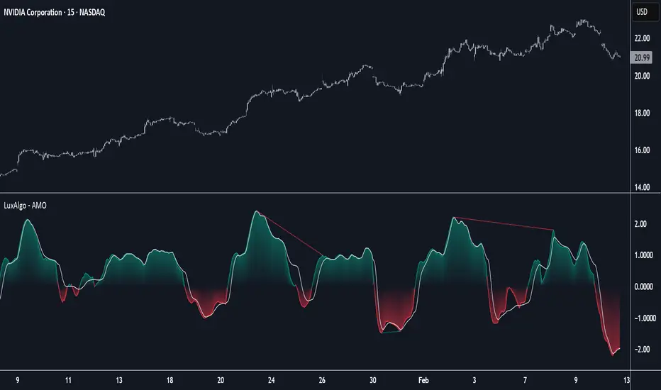
Machine Learning | Adaptive Trend Signals [Bitwardex]⚙️🧠Machine Learning | Adaptive Trend Signals
🔷Overview
Machine Learning | Adaptive Trend Signals is a Pine Script™ v6 indicator designed to visualize market trends and generate signals through a combination of volatility clustering, Gaussian smoothing, and adaptive trend calculations. Built as an overlay indicator, it integrates advanced techniques inspired by machine learning concepts, such as K-Means clustering, to adapt to changing market conditions. The script is highly customizable, includes a backtesting module, and supports alert conditions, making it suitable for traders exploring trend-based strategies and developers studying volatility-driven indicator design.
🔷Functionality
The indicator performs the following core functions:
• Volatility Clustering: Uses K-Means clustering to categorize market volatility into high, medium, and low states, adjusting trend sensitivity accordingly.
• Trend Calculation: Computes adaptive trend lines (SmartTrend) based on volatility-adjusted standard deviation, smoothed RSI, and ADX filters.
• Signal Generation: Identifies potential buy and sell points through trend line crossovers and directional confirmation.
• Backtesting Module: Tracks trade outcomes based on the SmartTrend3 value, displaying win rate and total trades.
• Visualization: Plots trend lines with gradient colors and optional signal markers (bullish 🐮 and bearish 🐻).
• Alerts: Provides configurable alerts for trend shifts and volatility state changes.
🔷Technical Methodology
Volatility Clustering with K-Means
The indicator employs a K-Means clustering algorithm to classify market volatility, measured via the Average True Range (ATR), into three distinct clusters:
• Data Collection: Gathers ATR values over a user-defined training period (default: 100 bars).
• Centroid Initialization: Sets initial centroids at the highest, lowest, and midpoint ATR values within the training period.
• Iterative Clustering: Assigns ATR data points to the nearest centroid, recalculates centroid means, and repeats until convergence.
• Dynamic Adjustment: Assigns a volatility state (high, medium, or low) based on the closest centroid, adjusting the trend factor (e.g., tighter for high volatility, wider for low volatility).
This approach allows the indicator to adapt its sensitivity to varying market conditions, providing a data-driven foundation for trend calculations.
🔷Gaussian Smoothing
To enhance signal clarity and reduce noise, the indicator applies Gaussian kernel smoothing to:
• RSI: Smooths the Relative Strength Index (calculated from OHLC4) to filter short-term fluctuations.
• SmartTrend: Smooths the primary trend line for a more stable output.
The Gaussian kernel uses a sigma value derived from the user-defined smoothing length, ensuring mathematically consistent noise reduction.
🔷SmartTrend Calculation
The pineSmartTrend function is the core of the indicator, producing three trend lines:
• SmartTrend: The primary trend line, calculated using a volatility-adjusted standard deviation, smoothed RSI, and ADX conditions.
• SmartTrend2: A secondary trend line with a wider factor (base factor * 1.382) for signal confirmation.
SmartTrend3: The average of SmartTrend and SmartTrend2, used for plotting and backtesting.
Key components of the calculation include:
• Dynamic Standard Deviation: Scales based on ATR relative to its 50-period smoothed average, with multipliers (1.0 to 1.4) applied according to volatility thresholds.
• RSI and ADX Filters: Requires RSI > 50 for bullish trends or < 50 for bearish trends, alongside ADX > 15 and rising to confirm trend strength.
Volatility-Adjusted Bands: Constructs upper and lower bands around price action, adjusted by the volatility cluster’s dynamic factor.
🔷Signal Generation
The generate_signals function generates signals as follows:
• Buy Signal: Triggered when SmartTrend crosses above SmartTrend2 and the price is above SmartTrend, with directional confirmation.
• Sell Signal: Triggered when SmartTrend crosses below SmartTrend2 and the price is below SmartTrend, with directional confirmation.
Directional Logic: Tracks trend direction to filter out conflicting signals, ensuring alignment with the broader market context.
Signals are visualized as small circles with bullish (🐮) or bearish (🐻) emojis, with an option to toggle visibility.
🔷Backtesting
The get_backtest function evaluates signal outcomes using the SmartTrend3 value (rather than closing prices) to align with the trend-based methodology.
It tracks:
• Total Trades: Counts completed long and short trades.
• Win Rate: Calculates the percentage of trades where SmartTrend3 moves favorably (higher for longs, lower for shorts).
Position Management: Closes opposite positions before opening new ones, simulating a single-position trading system.
Results are displayed in a table at the top-right of the chart, showing win rate and total trades. Note that backtest results reflect the indicator’s internal logic and should not be interpreted as predictive of real-world performance.
🔷Visualization and Alerts
• Trend Lines: SmartTrend3 is plotted with gradient colors reflecting trend direction and volatility cluster, accompanied by a secondary line for visual clarity.
• Signal Markers: Optional buy/sell signals are plotted as small circles with customizable colors.
• Alerts: Supports alerts for:
• Bullish and bearish trend shifts (confirmed on bar close).
Transitions to high, medium, or low volatility states.
🔷Input Parameters
• ATR Length (default: 14): Period for ATR calculation, used in volatility clustering.
• Period (default: 21): Common period for RSI, ADX, and standard deviation calculations.
• Base SmartTrend Factor (default: 2.0): Base multiplier for volatility-adjusted bands.
• SmartTrend Smoothing Length (default: 10): Length for Gaussian smoothing of the trend line.
• Show Buy/Sell Signals? (default: true): Enables/disables signal markers.
• Bullish/Bearish Color: Customizable colors for trend lines and signals.
🔷Usage Instructions
• Apply to Chart: Add the indicator to any TradingView chart.
• Configure Inputs: Adjust parameters to align with your trading style or market conditions (e.g., shorter ATR length for faster markets).
• Interpret Output:
• Trend Lines: Use SmartTrend3’s direction and color to gauge market bias.
• Signals: Monitor bullish (🐮) and bearish (🐻) markers for potential entry/exit points.
• Backtest Table: Review win rate and total trades to understand the indicator’s behavior in historical data.
• Set Alerts: Configure alerts for trend shifts or volatility changes to support manual or automated trading workflows.
• Combine with Analysis: Use the indicator alongside other tools or market context, as it is designed to complement, not replace, comprehensive analysis.
🔷Technical Notes
• Data Requirements: Requires at least 100 bars for accurate volatility clustering. Ensure sufficient historical data is loaded.
• Market Suitability: The indicator is designed for trend detection and may perform differently in ranging or volatile markets due to its reliance on RSI and ADX filters.
• Backtesting Scope: The backtest module uses SmartTrend3 values, which may differ from price-based outcomes. Results are for informational purposes only.
• Computational Intensity: The K-Means clustering and Gaussian smoothing may increase processing time on lower timeframes or with large datasets.
🔷For Developers
The script is modular, well-commented, encouraging reuse and modification with proper attribution.
Key functions include:
• gaussianSmooth: Applies Gaussian kernel smoothing to any data series.
• pineSmartTrend: Computes adaptive trend lines with volatility and momentum filters.
• getDynamicFactor: Adjusts trend sensitivity based on volatility clusters.
• get_backtest: Evaluates signal performance using SmartTrend3.
Developers can extend these functions for custom indicators or strategies, leveraging the volatility clustering and smoothing methodologies. The K-Means implementation is particularly useful for adaptive volatility analysis.
🔷Limitations
• The indicator is not predictive and should be used as part of a broader trading strategy.
• Performance varies by market, timeframe, and parameter settings, requiring user experimentation.
• Backtest results are based on historical data and internal logic, not real-world trading conditions.
• Volatility clustering assumes sufficient historical data; incomplete data may affect accuracy.
🔷Acknowledgments
Developed by Bitwardex, inspired by machine learning concepts and adaptive trading methodologies. Community feedback is welcome via TradingView’s platform.
🔷 Risk Disclaimer
Trading involves significant risks, and most traders may incur losses. Bitwardex AI Algo is provided for informational and educational purposes only and does not constitute financial advice or a recommendation to buy or sell any financial instrument . The signals, metrics, and features are tools for analysis and do not guarantee profits or specific outcomes. Past performance is not indicative of future results. Always conduct your own due diligence and consult a financial advisor before making trading decisions.

RSI-MACD Momentum Fusion Indicator(RMFI)📈 RSI-MACD Momentum Fusion Indicator (RMFI)
The RMFI combines the strengths of two RSI variants with a dynamically adaptive MACD module into a powerful momentum oscillator ranging from 0 to 100. The goal is to unify converging momentum information from different perspectives into a clear, weighted overall signal.
🔧 Core Features
RSI 1: Classic Wilder RSI, sensitive to short-term momentum.
RSI 2: Modified RSI based on normalized price movement ranges (Range Momentum).
MACD (3 Modes):
Standardized (min/max-based)
Fully adaptive (Z-score normalization)
50% adaptive (hybrid weighting of both approaches)
Dynamic MACD mode selection (optional): Automatic switching of MACD normalization based on volatility levels (ATR-based).
Signal Line: Smoothed average of all components to visualize momentum trends and crossovers.
🎯 Visualization
Clear separation of overbought (>70) and oversold (<30) zones with color highlighting.
Different colors based on the dynamic MACD mode – visually indicates how strongly the market adapts to volatility.
⚙️ Recommended Use
Ideal for trend following, divergence confirmation (with external divergence logic), and momentum reversals.
Particularly effective in volatile markets, as the MACD component adaptively responds to instability.
© champtrades
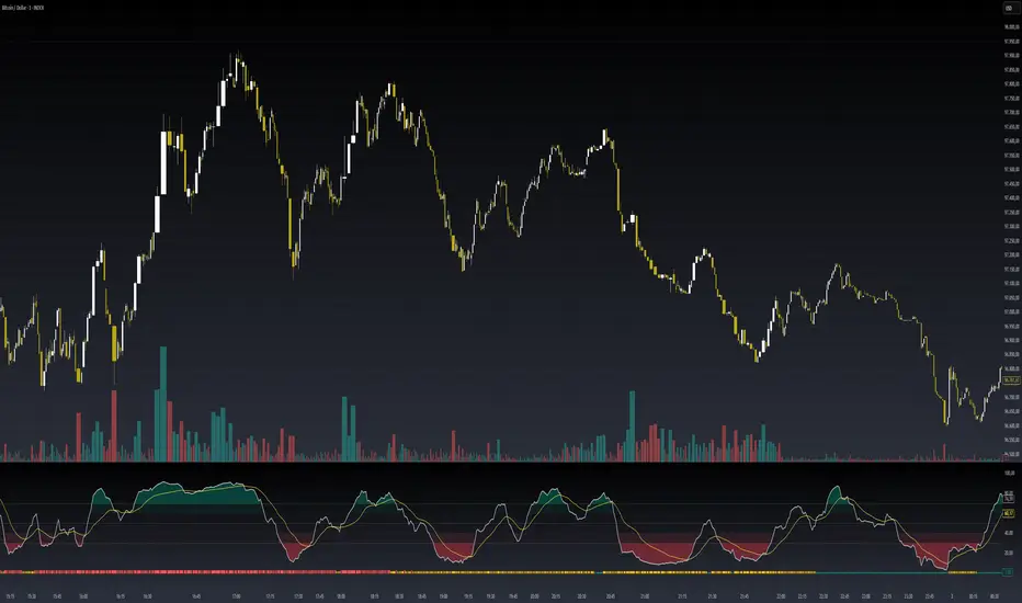
Adaptable Relative Momentum Index [ParadoxAlgo]The Adaptable Relative Momentum Index (RMI) by ParadoxAlgo is an advanced momentum-based indicator that builds upon the well-known RSI (Relative Strength Index) concept by introducing a customizable momentum length. This indicator measures price momentum over a specified number of periods and applies a Rolling Moving Average (RMA) to both the positive and negative price changes. The result is a versatile tool that can help traders gauge the strength of a trend, pinpoint overbought/oversold levels, and potentially identify breakout opportunities.
⸻
Smart Configuration Feature
What sets this version of the RMI apart is ParadoxAlgo’s exclusive “Smart Configuration” functionality. Instead of manually adjusting parameters, traders can simply select their Asset Class (e.g., Stocks, Forex, Futures/Indices, Crypto, Commodities) and Trading Style (e.g., Scalping, Day Trading, Swing Trading, Short-Term Investing, Long-Term Investing). Based on these selections, the indicator automatically optimizes its core parameters:
• Length – The period over which the price changes are smoothed.
• Momentum Length – The number of bars used to calculate the price change.
By automating this process, users save time on tedious trial-and-error adjustments, ensuring that the RMI’s settings are tailored to the characteristics of specific markets and personal trading horizons.
⸻
Key Features & Benefits
1. Momentum-Based Insights
• Uses RMA to smooth price movements, helping identify shifts in market momentum more clearly than a basic RSI.
• Enhanced adaptability for a wide range of asset classes and time horizons.
2. Simple Yet Powerful Configuration
• Smart Configuration automatically sets optimal parameter values for each combination of asset class and trading style.
• Eliminates guesswork and manual recalibration when switching between markets or timeframes.
3. Overbought & Oversold Visualization
• Integrated highlight zones mark potential overbought and oversold extremes (default at 80 and 20).
• Optional breakout highlighting draws attention to times when the indicator crosses these key thresholds, helping spot possible entry or exit signals.
4. Intuitive Design & Ease of Use
• Clean plotting and color-coded signal lines make it easy to interpret bullish or bearish shifts in momentum.
• Straightforward dropdown menus keep the interface user-friendly, even for novice traders.
⸻
Practical Applications
• Early Trend Detection: Spot emerging trends when the RMI transitions from oversold to higher levels or vice versa.
• Breakout Confirmation: Confirm potential breakout trades by tracking overbought/oversold breakouts alongside other technical signals.
• Support/Resistance Confluence: Combine RMI signals with horizontal support/resistance levels to reinforce trade decisions.
• Trade Timing: Quickly gauge when momentum could be shifting, helping you time entries and exits more effectively.
⸻
Disclaimer
As with any technical indicator, the Adaptable Relative Momentum Index should be used as part of a broader trading strategy that includes risk management, fundamental analysis, and other forms of technical confirmation. Past performance does not guarantee future results.
⸻
Enjoy using the Adaptable RMI and experience a more streamlined, flexible approach to momentum analysis. Feel free to explore different asset classes and trading styles to discover which configurations resonate best with your unique trading preferences.

Ehlers Adaptive Trend Indicator [Alpha Extract]Ehlers Adaptive Trend Indicator
The Ehlers Adaptive Trend Indicator combines Ehlers' advanced digital signal processing techniques with dynamic volatility bands to identify robust trend conditions and potential reversals. This powerful tool helps traders visualize trend strength, adaptive support/resistance levels, and momentum shifts across various market conditions.
🔶 CALCULATION
The indicator employs a sophisticated adaptive algorithm that responds to changing market conditions:
• Ehlers Filter : Calculates a weighted average based on momentum differences to create an adaptive trend baseline.
• Dynamic Bands : Volatility-adjusted bands that expand and contract based on recent price action.
• Trend Level : A dynamic support/resistance level that adapts to the current trend direction.
• Smoothed Volatility : Market volatility measured and smoothed to provide reliable band width.
Formula:
• Ehlers Basis = Weighted average of price, with weights determined by momentum differences
• Volatility = Standard deviation of price over Ehlers Length period
• Smoothed Volatility = EMA of volatility over Smoothing Length
• Upper Band = Ehlers Basis + Smoothed Volatility × Sensitivity
• Lower Band = Ehlers Basis - Smoothed Volatility × Sensitivity
• Trend Level = Adaptive support in uptrends, resistance in downtrends
🔶 DETAILS
Visual Features :
• Ehlers Basis Line (Yellow): The core adaptive trend reference that serves as the primary trend indicator.
• Trend Level Line (Dynamic Color): Changes between green (bullish) and red (bearish) based on the current trend state.
• Fill Areas : Transparent green fill during bullish trends and transparent red fill during bearish trends for clear visual identification.
• Bar Coloring : Optional price bar coloring that reflects the current trend direction for enhanced visualization.
Interpretation :
• **Bullish Signal**: Price crosses above the upper band, triggering a trend change with the Trend Level becoming dynamic support.
• **Bearish Signal**: Price drops below the lower band, confirming a trend change with the Trend Level becoming dynamic resistance.
• **Trend Continuation**: Trend Level rises in bullish markets and falls in bearish markets, providing adaptive trailing support/resistance.
🔶 EXAMPLES
The chart demonstrates:
• Bullish Trend Identification : When price breaks above the upper band, the indicator shifts to bullish mode with green trend level and fill.
• Bearish Trend Identification : When price falls below the lower band, the indicator shifts to bearish mode with red trend level and fill.
• Trend Persistence : Trend Level adapts to market movement, rising during uptrends to provide dynamic support and falling during downtrends to act as resistance.
Example Snapshots :
• During a strong uptrend, the Trend Level continuously adjusts upward, keeping traders in the trend while filtering out minor retracements.
• During trend reversals, clear color changes and Trend Level shifts provide early warning of potential direction changes.
🔶 SETTINGS
Customization Options :
• Ehlers Length (p1) (Default: 30): Controls the primary adaptive calculation period, balancing responsiveness with stability.
• Momentum Length (p2) (Default: 25): Determines the lag for momentum calculations used in the adaptive weighting.
• Smoothing Length (Default: 10): Adjusts the volatility smoothing period—higher values provide more stable bands.
• Sensitivity (Default: 1.0): Multiplier for band width—higher values increase distance between bands, lower values tighten them.
• Visual Settings : Customizable colors for bullish and bearish trends, basis line, and optional bar coloring.
The Ehlers Adaptive Trend Indicator combines John Ehlers' digital signal processing expertise with modern volatility analysis to create a robust trend-following system that adapts to changing market conditions, helping traders stay on the right side of the market.