Drawdown + Labels BINANCE:BTCUSDT
Indicador de reducciones de precio con etiqueta.
El indicador toma por defecto el valor máximo histórico y a partir de ese valor realiza los siguientes cálculos:
Reducción del 50% = Máximo Histórico*(50/100)
Reducción del 60% = Máximo Histórico*(40/100)
Reducción del 70% = Máximo Histórico*(30/100)
Reducción del 80% = Máximo Histórico*(20/100)
Reducción del 90% = Máximo Histórico*(10/100)
En el grafico se mostrará una etiqueta a la derecha por defecto, el valor que corresponde a cada reducción.
Ejemplo:
Fecha: 04 de Enero de 2022
Máximo Histórico de BTC = $ 69,000 (Línea color Naranja)
Reducción del 50% = $ 34,500 (Línea color Morada)
Reducción del 60% = $ 27,600 (Línea color Marrón)
Reducción del 70% = $ 20,700 (Línea color Verde)
Reducción del 80% = $ 13,800 (Línea color Roja)
Reducción del 90% = $ 6,900 (Línea color Aqua)
Reducción del 100% = $ 0 (Línea color Negro)
Espero les ayude, saludos.
In den Scripts nach "市值大于100亿且市盈率小于5的股票最新数据更新时间" suchen

Portfolio Backtester Engine█ OVERVIEW
Portfolio Backtester Engine (PBTE). This tool will allow you to backtest strategies across multiple securities at once. Allowing you to easier understand if your strategy is robust. If you are familiar with the PineCoders backtesting engine , then you will find this indicator pleasant to work with as it is an adaptation based on that work. Much of the functionality has been kept the same, or enhanced, with some minor adjustments I made on the account of creating a more subjectively intuitive tool.
█ HISTORY
The original purpose of the backtesting engine (`BTE`) was to bridge the gap between strategies and studies . Previously, strategies did not contain the ability to send alerts, but were necessary for backtesting. Studies on the other hand were necessary for sending alerts, but could not provide backtesting results . Often, traders would have to manage two separate Pine scripts to take advantage of each feature, this was less than ideal.
The `BTE` published by PineCoders offered a solution to this issue by generating backtesting results under the context of a study(). This allowed traders to backtest their strategy and simultaneously generate alerts for automated trading, thus eliminating the need for a separate strategy() script (though, even converting the engine to a strategy was made simple by the PineCoders!).
Fast forward a couple years and PineScript evolved beyond these issues and alerts were introduced into strategies. The BTE was not quite as necessary anymore, but is still extremely useful as it contains extra features and data not found under the strategy() context. Below is an excerpt of features contained by the BTE:
"""
More than `40` built-in strategies,
Customizable components,
Coupling with your own external indicator,
Simple conversion from Study to Strategy modes,
Post-Exit analysis to search for alternate trade outcomes,
Use of the Data Window to show detailed bar by bar trade information and global statistics, including some not provided by TV backtesting,
Plotting of reminders and generation of alerts on in-trade events.
"""
Before I go any further, I want to be clear that the BTE is STILL a good tool and it is STILL very useful. The Portfolio Backtesting Engine I am introducing is only a tangental advancement and not to be confused as a replacement, this tool would not have been possible without the `BTE`.
█ THE PROBLEM
Most strategies built in Pine are limited by one thing. Data. Backtesting should be a rigorous process and researchers should examine the performance of their strategy across all market regimes; that includes, bullish and bearish markets, ranging markets, low volatility and high volatility. Depending on your TV subscription The Pine Engine is limited to 5k-20k historical bars available for backtesting, which can often leave the strategy results wanting. As a general rule of thumb, strategies should be tested across a quantity of historical bars which will allow for at least 100 trades. In many cases, the lack of historical bars available for backtesting and frequency of the strategy signals produces less than 100 trades, rendering your strategy results inconclusive.
█ THE SOLUTION
In order to be confident that we have a robust strategy we must test it across all market regimes and we must have over 100 trades. To do this effectively, researchers can use the Portfolio Backtesting Engine (PBTE).
By testing a strategy across a carefully selected portfolio of securities, researchers can now gather 5k-20k historical bars per security! Currently, the PTBE allows up to 5 securities, which amounts to 25k-100k historical bars.
█ HOW TO USE
1 — Add the indicator to your chart.
• Confirm inputs. These will be the most important initial values which you can change later by clicking the gear icon ⚙ and opening up the settings of the indicator.
2 — Select a portfolio.
• You will want to spend some time carefully selecting a portfolio of securities.
• Each security should be uncorrelated.
• The entire portfolio should contain a mix of different market regimes.
You should understand that strategies generally take advantage of one particular type of market regime. (trending, ranging, low/high volatility)
For example, the default RSI strategy is typically advantageous during ranging markets, whereas a typical moving average crossover strategy is advantageous in trending markets.
If you were to use the standard RSI strategy during a trending market, you might be selling when you should be buying.
Similarily, if you use an SMA crossover during a ranging market, you will find that the MA's may produce many false signals.
Even if you build a strategy that is designed to be used only in a trending market, it is still best to select a portfolio of all market regimes
as you will be able to test how your strategy will perform when the market does something unexpected.
3 — Test a built-in strategy or add your own.
• Navigate to gear icon ⚙ (settings) of strategy.
• Choose your options.
• Select a Main Entry Strat and Alternate Entry Strat .
• If you want to add your own strategy, you will need to modify the source code and follow the built-in example.
• You will only need to generate (buy 1 / sell -1/ neutral 0) signals.
• Select a Filter , by default these are all off.
• Select an Entry Stop - This will be your stop loss placed at the trade entry.
• Select Pyamiding - This will allow you to stack positions. By default this is off.
• Select Hard Exits - You can also think of these as Take Profits.
• Let the strategy run and take note of the display tables results.
• Portfolio - Shows each security.
• The strategy runs on each asset in your portfolio.
• The initial capital is equally distributed across each security.
So if you have 5 securities and a starting capital of 100,000$ then each security will run the strategy starting with 20,000$
The total row will aggregate the results on a bar by bar basis showing the total results of your initial capital.
• Net Profit (NP) - Shows profitability.
• Number of Trades (#T) - Shows # of trades taken during backtesting period.
• Typically will want to see this number greater than 100 on the "Total" row.
• Average Trade Length (ATL) - Shows average # of days in a trade.
• Maximum Drawdown (MD ) - Max peak-to-valley equity drawdown during backtesting period.
• This number defines the minimum amount of capital required to trade the system.
• Typically, this shouldn’t be lower than 34% and we will want to allow for at least 50% beyond this number.
• Maximum Loss (ML) - Shows largest loss experienced on a per-trade basis.
• Normally, don’t want to exceed more than 1-2 % of equity.
• Maximum Drawdown Duration (MDD) - The longest duration of a drawdown in equity prior to a new equity peak.
• This number is important to help us psychologically understand how long we can expect to wait for a new peak in account equity.
• Maximum Consecutive Losses (MCL) - The max consecutive losses endured throughout the backtesting period.
• Another important metric for trader psychology, this will help you understand how many losses you should be prepared to handle.
• Profit to Maximum Drawdown (P:MD) - A ratio for the average profit to the maximum drawdown.
• The higher the ratio is, the better. Large profits and small losses contribute to a good PMD.
• This metric allows us to examine the profit with respect to risk.
• Profit Loss Ratio (P:L) - Average profit over the average loss.
• Typically this number should be higher in trend following systems.
• Mean reversion systems show lower values, but compensate with a better win %.
• Percent Winners (% W) - The percentage of winning trades.
• Trend systems will usually have lower win percentages, since statistically the market is only trending roughly 30% of the time.
• Mean reversion systems typically should have a high % W.
• Time Percentage (Time %) - The amount of time that the system has an open position.
• The more time you are in the market, the more you are exposed to market risk, not to mention you could be using that money for something else right?
• Return on Investment (ROI) - Your Net Profit over your initial investment, represented as a percentage.
• You want this number to be positive and high.
• Open Profit (OP) - If the strategy has any open positions, the floating value will be represented here.
• Trading Days (TD) - An important metric showing how many days the strategy was active.
• This is good to know and will be valuable in understanding how long you will need to run this strategy in order to achieve results.
█ FEATURES
These are additional features that extend the original `BTE` features.
- Portfolio backtesting.
- Color coded performance results.
- Circuit Breakers that will stop trading.
- Position reversals on exit. (Simulating the function of always in the market. Similar to strategy.entry functionality)
- Whipsaw Filter
- Moving Average Filter
- Minimum Change Filter
- % Gain Equity Exit
- Popular strategies, (MACD, MA cross, supertrend)
Below are features that were excluded from the original `BTE`
- 2 stage in-trade stops with kick-in rules (This was a subjective decision to remove. I found it to be complex and thwarted my use of the `BTE` for some time.)
- Simple conversion from Study to Strategy modes. (Not possible with multiple securities)
- Coupling with your own external indicator (Not really practical to use with multiple securities, but could be used if signals were generated based on some indicator which was not based on the current chart)
- Use of the Data Window to show detailed bar by bar trade information and global statistics.
- Post Exit Analysis.
- Plotting of reminders and generation of alerts on in-trade events.
- Alerts (These may be added in the future by request when I find the time.)
█ THANKS
The whole PineCoders team for all their shared knowledge and original publication of the BTE and Richard Weismann for his ideas on building robust strategies.
═════════════════════════════════════════════════════════════════════════

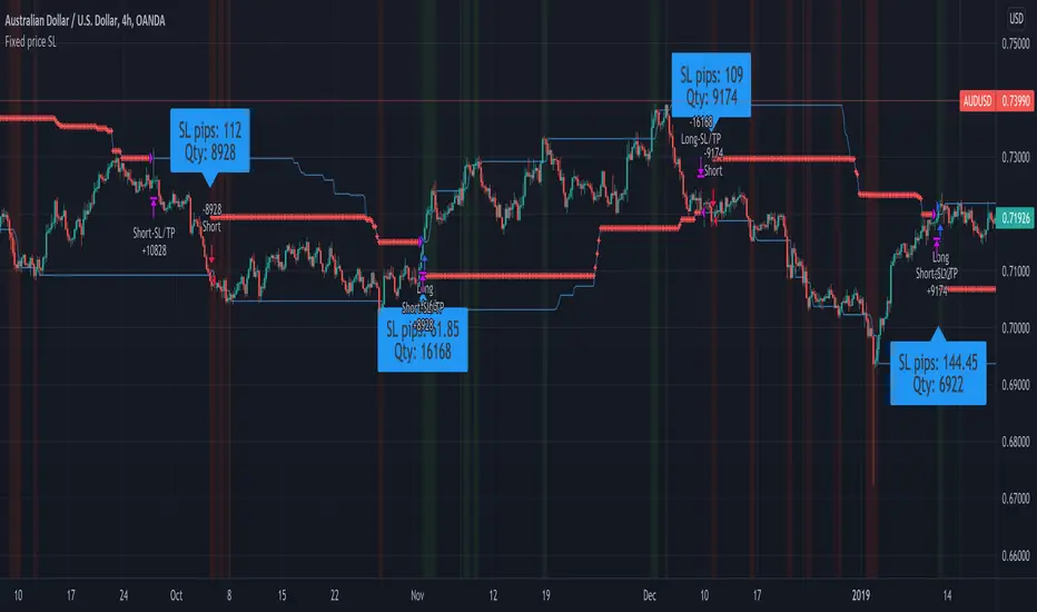
Fixed price Stop Loss [Takazudo]This strategy is a demo for fixed price stop loss.
This strategy enables you to specify fixed price stop loss. Let's say your deposit is USD. When you trade EURCAD, you need to specify the quantity for trade. Here comes three chances for trade.
A: SL pips: 500
B: SL pips: 200
C: SL pips: 100
In these trade, the risk is different for each. ABC risk ratio is 5:2:1. And, you cannot know how much to lose if the price hits the stop loss. This is a huge problem.
With this strategy, You can specify the fixed risk price for each trade. If you specify 100 USD for the risk, this strategy calculates how much quantity to buy or sell for each entry. In the case above, this strategy guides you how much quantity to buy or sell like below.
A: 2,000 qty (SL: 500pips)
B: 5,000 qty (SL: 200pips)
C: 10,000 qty (SL: 100pips)
If you make entries with those quantity and the price hits the stop loss, You will lose the money like below.
A: 100 USD
B: 100 USD
C: 100 USD
This is what this script does. Fixed price SL.
I tested this caliculation for OANDA's main 28 currency pairs forex listed below.
AUDUSD, EURUSD, GBPUSD, NZDUSD, USDCAD, USDCHF, USDJPY, AUDCAD, AUDCHF, AUDJPY, AUDNZD, CADCHF, CADJPY, CHFJPY, EURAUD, EURCAD, EURCHF, EURGBP, EURJPY, EURNZD, GBPAUD, GBPCAD, GBPCHF, GBPJPY, GBPNZD, NZDCAD, NZDCHF, NZDJPY
I may add more pairs later.
Note: The entry strategy in this script is not intented to win. Check the result. Be careful.
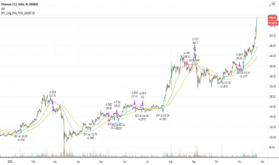
BTC and ETH Long strategy - version 2I wrote my first article in May 2020. See below
BTC and ETH Long strategy - version1
After 6 months, it is now time to check the result of my script for the last 6 months.
XBTUSD (4H): 14/05/2020 --> 22/11/2020 = +78% in 4 trades
ETHXBT (4H): 14/05/2020 --> 22/11/2020 = +21% in 9 trades
ETHUSD (4H): 14/05/2020 --> 22/11/2020 = +90% in 6 trades
Using the signals from this strategy to trade manually has shown that this was a bit frustrating because of the low rate of winning trades.
If you have to enter 100 trades and see 75% of them failing and 25% winning, this is frustrating. For sure the strategy makes good money but it is difficult to hold this mentality.
So, I have reviewed and modified it to get a higher winning rate.
After few days of work, tests and validation, I managed to get a wining rate close to 60%.
The key element was also to decrease the number of trades by using a higher time frame. (4H candles instead of 2H candles).
- Entry in position is based on
MACD, EMA (20), SMA (100), SMA (200) moving up
AND EMA (20) > SMA (100)
AND SMA (100) > SMA (200)
- Exit the position if: Stoploss is reached OR EMA (20) crossUnder SMA (100)
The goal of this new script is to be able to follow the signals manually and only make few trades per years.
I have also validated it against some other altcoins where some are giving very good results.
Here are some results for 2020 (from 01/01/2020 until now (22/11/2020). Those results are the one I get when using 4H candles.
ETH/USD: +144% in 8 trades.
BTC/USD: +120% in 7 trades.
ETH/BTC: +33% in 9 trades.
ICX/USD: +123% in 10 trades.
LINK/USD: +155% in 11 trades.
MLN/USD: +388% in 8 trades.
ADA/USD: +180% in 7 trades.
LINK/BTC: +97% in 10 trades.
The best is that above results are without considering compound effect. If you re-invest all gains done in each new trade, this will give you the below results :)
ETH/USD: +189% in 8 trades.
BTC/USD: +260% in 7 trades.
ETH/BTC: +29% in 9 trades.
ICX/USD: +112% in 10 trades.
LINK/USD: +222% in 11 trades.
MLN/USD: +793% in 8 trades.
ADA/USD: +319% in 7 trades.
LINK/BTC: +103% in 10 trades.
As you can see, the results are good and the number of trades for 11 months is not big, which allows the trader to place orders manually.
But still, I'm lazy :), so, I have also coded this strategy in HaasScript language which allows you to automate this strategy using the HaasOnline software specialized in automated crypto trading.
I hope that this strategy will give you ideas or will be the starting point for your own strategy.
Let me know if you need more details.
BTC and ETH Long strategy - version 1I will start with a small introduction about myself. I'm now trading cryto currencies manually for almost 2 years. I decided to start after watching a documentary on the TV showing people who made big money during the Bitcoin pump which happened at the end of 2017.
The next day, I asked myself "Why should I not give it a try and learn how to trade".
This was in February 2018 and the price of Bitcoin was around 11500USD.
I didn't know how to trade. In fact, I didn't know the trading industry at all.
So, my first step into trading was to open an account with a broken. Then I directly bought 200$ worst of BTC . At that time, I saw the graph and thought "This can only go back in the upward direction!" :)
I didn't know anything about Stop loss, Take profit and Risk management.
Today, almost 2 years after, I think that I know how to trade and can also confirm that I still hold this bag of 200$ of bitcoin from 2018 :)
I did spend the 2 last years to learn technical analysis , risk management and leverage trading.
Today (14/05/2020), I know what I'm doing and I'm happy to see that the 2 last years have been positive in terms of gains. Of course, I did not make crazy money with my saving but at least I made more than if I would have kept it in my bank account.
Even if I like trading, I have a full time job which requires my full energy and lots of focus, so, the biggest problem I had is that I didn't have enough time to look at the charts.
Also, I realized that sometimes, neither technical analysis , nor fundamentals worked with crypto currency (at least for short time trading). So, as I have a developer background I decided to try to have a look at algo trading.
The goal for me was neither to make complex algos nor to beat the market but just to automate my trading with simple bot catching the big waves.
I then started to take a look at TV pine script and played with it.
I did my first LONG script in February 2020 to Long the BTC Market. It has some limitations but works well enough for me for the time being. Even if the real trades will bring me half of what the back testing shows, this will still be a lot more than what I was used to win during the last 2 years with my manual trading.
So, here we are! Below you will find some details about my first LONG script. I'm happy to share it with you.
Feel free to play with it, give your comments and bring improvements to it.
But please note that it only works fine with the candle size and crypto pair that I have mentioned below. If you use other settings this algo might loose money!
- Crypto pairs : XBTUSD and ETHXBT
- Candle size: 2 Hours
- Indicator used: Volatility , MACD (12, 26, 7), SMA (100), SMA (200), EMA (20)
- Default StopLoss: -1.5%
- Entry in position if: Volatility < 2%
AND MACD moving up
AND AME (20) moving up
AND SMA (100) moving up
AND SMA (200) moving up
AND EMA (20) > SAM (100)
AND SMA (100) > SMA (200)
- Exit the postion if: Stoploss is reached
OR EMA (20) crossUnder SMA (100)
Here is a summary of the results for this script:
XBTUSD : 01/01/2019 --> 14/05/2020 = +107%
ETHXBT : 01/01/2019 --> 14/05/2020 = +39%
ETHUSD : 01/01/2019 --> 14/05/2020 = +112%
It is far away from being perfect. There are still plenty of things which can be done to improve it but I just wanted to share it :) .
Enjoy playing with it....

Fischy Bands (multiple periods)Just a quick way to have multiple periods. Coded at (14,50,100,200,400,600,800). Feel free to tweak it. Default is all on, obviously not as usable! Try just using 14, and 50.
This was generated with javascript for easy templating.
Source:
```
const periods = ;
const generate = (period) => {
const template = `
= bandFor(${period})
plot(b${period}, color=colorFor(${period}, b${period}), linewidth=${periods.indexOf(period)+1}, title="BB ${period} Basis", transp=show${period}TransparencyLine)
pb${period}Upper = plot(b${period}Upper, color=colorFor(${period}, b${period}), linewidth=${periods.indexOf(period)+1}, title="BB ${period} Upper", transp=show${period}TransparencyLine)
pb${period}Lower = plot(b${period}Lower, color=colorFor(${period}, b${period}), linewidth=${periods.indexOf(period)+1}, title="BB ${period} Lower", transp=show${period}TransparencyLine)
fill(pb${period}Upper, pb${period}Lower, color=colorFor(${period}, b${period}), transp=show${period}TransparencyFill)`
console.log(template);
}
console.log(`//@version=4
study(shorttitle="Fischy BB", title="Fischy Bands", overlay=true)
stdm = input(1.25, title="stdev")
bandFor(length) =>
src = hlc3
mult = stdm
basis = sma(src, length)
dev = mult * stdev(src, length)
upper = basis + dev
lower = basis - dev
`);
periods.forEach(e => console.log(`show${e} = input(title="Show ${e}?", type=input.bool, defval=true)`));
periods.forEach(e => console.log(`show${e}TransparencyLine = show${e} ? 20 : 100`));
periods.forEach(e => console.log(`show${e}TransparencyFill = show${e} ? 80 : 100`));
console.log('\n');
console.log(`colorFor(period, series) =>
c = period == 14 ? color.white :
period == 50 ? color.aqua :
period == 100 ? color.orange :
period == 200 ? color.purple :
period == 400 ? color.lime :
period == 600 ? color.yellow :
period == 800 ? color.orange :
color.black
c
`);
periods.forEach(e => generate(e))
```

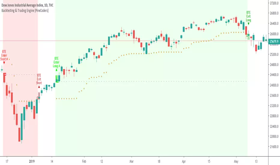
Backtesting & Trading Engine [PineCoders]The PineCoders Backtesting and Trading Engine is a sophisticated framework with hybrid code that can run as a study to generate alerts for automated or discretionary trading while simultaneously providing backtest results. It can also easily be converted to a TradingView strategy in order to run TV backtesting. The Engine comes with many built-in strats for entries, filters, stops and exits, but you can also add you own.
If, like any self-respecting strategy modeler should, you spend a reasonable amount of time constantly researching new strategies and tinkering, our hope is that the Engine will become your inseparable go-to tool to test the validity of your creations, as once your tests are conclusive, you will be able to run this code as a study to generate the alerts required to put it in real-world use, whether for discretionary trading or to interface with an execution bot/app. You may also find the backtesting results the Engine produces in study mode enough for your needs and spend most of your time there, only occasionally converting to strategy mode in order to backtest using TV backtesting.
As you will quickly grasp when you bring up this script’s Settings, this is a complex tool. While you will be able to see results very quickly by just putting it on a chart and using its built-in strategies, in order to reap the full benefits of the PineCoders Engine, you will need to invest the time required to understand the subtleties involved in putting all its potential into play.
Disclaimer: use the Engine at your own risk.
Before we delve in more detail, here’s a bird’s eye view of the Engine’s features:
More than 40 built-in strategies,
Customizable components,
Coupling with your own external indicator,
Simple conversion from Study to Strategy modes,
Post-Exit analysis to search for alternate trade outcomes,
Use of the Data Window to show detailed bar by bar trade information and global statistics, including some not provided by TV backtesting,
Plotting of reminders and generation of alerts on in-trade events.
By combining your own strats to the built-in strats supplied with the Engine, and then tuning the numerous options and parameters in the Inputs dialog box, you will be able to play what-if scenarios from an infinite number of permutations.
USE CASES
You have written an indicator that provides an entry strat but it’s missing other components like a filter and a stop strategy. You add a plot in your indicator that respects the Engine’s External Signal Protocol, connect it to the Engine by simply selecting your indicator’s plot name in the Engine’s Settings/Inputs and then run tests on different combinations of entry stops, in-trade stops and profit taking strats to find out which one produces the best results with your entry strat.
You are building a complex strategy that you will want to run as an indicator generating alerts to be sent to a third-party execution bot. You insert your code in the Engine’s modules and leverage its trade management code to quickly move your strategy into production.
You have many different filters and want to explore results using them separately or in combination. Integrate the filter code in the Engine and run through different permutations or hook up your filtering through the external input and control your filter combos from your indicator.
You are tweaking the parameters of your entry, filter or stop strat. You integrate it in the Engine and evaluate its performance using the Engine’s statistics.
You always wondered what results a random entry strat would yield on your markets. You use the Engine’s built-in random entry strat and test it using different combinations of filters, stop and exit strats.
You want to evaluate the impact of fees and slippage on your strategy. You use the Engine’s inputs to play with different values and get immediate feedback in the detailed numbers provided in the Data Window.
You just want to inspect the individual trades your strategy generates. You include it in the Engine and then inspect trades visually on your charts, looking at the numbers in the Data Window as you move your cursor around.
You have never written a production-grade strategy and you want to learn how. Inspect the code in the Engine; you will find essential components typical of what is being used in actual trading systems.
You have run your system for a while and have compiled actual slippage information and your broker/exchange has updated his fees schedule. You enter the information in the Engine and run it on your markets to see the impact this has on your results.
FEATURES
Before going into the detail of the Inputs and the Data Window numbers, here’s a more detailed overview of the Engine’s features.
Built-in strats
The engine comes with more than 40 pre-coded strategies for the following standard system components:
Entries,
Filters,
Entry stops,
2 stage in-trade stops with kick-in rules,
Pyramiding rules,
Hard exits.
While some of the filter and stop strats provided may be useful in production-quality systems, you will not devise crazy profit-generating systems using only the entry strats supplied; that part is still up to you, as will be finding the elusive combination of components that makes winning systems. The Engine will, however, provide you with a solid foundation where all the trade management nitty-gritty is handled for you. By binding your custom strats to the Engine, you will be able to build reliable systems of the best quality currently allowed on the TV platform.
On-chart trade information
As you move over the bars in a trade, you will see trade numbers in the Data Window change at each bar. The engine calculates the P&L at every bar, including slippage and fees that would be incurred were the trade exited at that bar’s close. If the trade includes pyramided entries, those will be taken into account as well, although for those, final fees and slippage are only calculated at the trade’s exit.
You can also see on-chart markers for the entry level, stop positions, in-trade special events and entries/exits (you will want to disable these when using the Engine in strategy mode to see TV backtesting results).
Customization
You can couple your own strats to the Engine in two ways:
1. By inserting your own code in the Engine’s different modules. The modular design should enable you to do so with minimal effort by following the instructions in the code.
2. By linking an external indicator to the engine. After making the proper selections in the engine’s Settings and providing values respecting the engine’s protocol, your external indicator can, when the Engine is used in Indicator mode only:
Tell the engine when to enter long or short trades, but let the engine’s in-trade stop and exit strats manage the exits,
Signal both entries and exits,
Provide an entry stop along with your entry signal,
Filter other entry signals generated by any of the engine’s entry strats.
Conversion from strategy to study
TradingView strategies are required to backtest using the TradingView backtesting feature, but if you want to generate alerts with your script, whether for automated trading or just to trigger alerts that you will use in discretionary trading, your code has to run as a study since, for the time being, strategies can’t generate alerts. From hereon we will use indicator as a synonym for study.
Unless you want to maintain two code bases, you will need hybrid code that easily flips between strategy and indicator modes, and your code will need to restrict its use of strategy() calls and their arguments if it’s going to be able to run both as an indicator and a strategy using the same trade logic. That’s one of the benefits of using this Engine. Once you will have entered your own strats in the Engine, it will be a matter of commenting/uncommenting only four lines of code to flip between indicator and strategy modes in a matter of seconds.
Additionally, even when running in Indicator mode, the Engine will still provide you with precious numbers on your individual trades and global results, some of which are not available with normal TradingView backtesting.
Post-Exit Analysis for alternate outcomes (PEA)
While typical backtesting shows results of trade outcomes, PEA focuses on what could have happened after the exit. The intention is to help traders get an idea of the opportunity/risk in the bars following the trade in order to evaluate if their exit strategies are too aggressive or conservative.
After a trade is exited, the Engine’s PEA module continues analyzing outcomes for a user-defined quantity of bars. It identifies the maximum opportunity and risk available in that space, and calculates the drawdown required to reach the highest opportunity level post-exit, while recording the number of bars to that point.
Typically, if you can’t find opportunity greater than 1X past your trade using a few different reasonable lengths of PEA, your strategy is doing pretty good at capturing opportunity. Remember that 100% of opportunity is never capturable. If, however, PEA was finding post-trade maximum opportunity of 3 or 4X with average drawdowns of 0.3 to those areas, this could be a clue revealing your system is exiting trades prematurely. To analyze PEA numbers, you can uncomment complete sets of plots in the Plot module to reveal detailed global and individual PEA numbers.
Statistics
The Engine provides stats on your trades that TV backtesting does not provide, such as:
Average Profitability Per Trade (APPT), aka statistical expectancy, a crucial value.
APPT per bar,
Average stop size,
Traded volume .
It also shows you on a trade-by-trade basis, on-going individual trade results and data.
In-trade events
In-trade events can plot reminders and trigger alerts when they occur. The built-in events are:
Price approaching stop,
Possible tops/bottoms,
Large stop movement (for discretionary trading where stop is moved manually),
Large price movements.
Slippage and Fees
Even when running in indicator mode, the Engine allows for slippage and fees to be included in the logic and test results.
Alerts
The alert creation mechanism allows you to configure alerts on any combination of the normal or pyramided entries, exits and in-trade events.
Backtesting results
A few words on the numbers calculated in the Engine. Priority is given to numbers not shown in TV backtesting, as you can readily convert the script to a strategy if you need them.
We have chosen to focus on numbers expressing results relative to X (the trade’s risk) rather than in absolute currency numbers or in other more conventional but less useful ways. For example, most of the individual trade results are not shown in percentages, as this unit of measure is often less meaningful than those expressed in units of risk (X). A trade that closes with a +25% result, for example, is a poor outcome if it was entered with a -50% stop. Expressed in X, this trade’s P&L becomes 0.5, which provides much better insight into the trade’s outcome. A trade that closes with a P&L of +2X has earned twice the risk incurred upon entry, which would represent a pre-trade risk:reward ratio of 2.
The way to go about it when you think in X’s and that you adopt the sound risk management policy to risk a fixed percentage of your account on each trade is to equate a currency value to a unit of X. E.g. your account is 10K USD and you decide you will risk a maximum of 1% of it on each trade. That means your unit of X for each trade is worth 100 USD. If your APPT is 2X, this means every time you risk 100 USD in a trade, you can expect to make, on average, 200 USD.
By presenting results this way, we hope that the Engine’s statistics will appeal to those cognisant of sound risk management strategies, while gently leading traders who aren’t, towards them.
We trade to turn in tangible profits of course, so at some point currency must come into play. Accordingly, some values such as equity, P&L, slippage and fees are expressed in currency.
Many of the usual numbers shown in TV backtests are nonetheless available, but they have been commented out in the Engine’s Plot module.
Position sizing and risk management
All good system designers understand that optimal risk management is at the very heart of all winning strategies. The risk in a trade is defined by the fraction of current equity represented by the amplitude of the stop, so in order to manage risk optimally on each trade, position size should adjust to the stop’s amplitude. Systems that enter trades with a fixed stop amplitude can get away with calculating position size as a fixed percentage of current equity. In the context of a test run where equity varies, what represents a fixed amount of risk translates into different currency values.
Dynamically adjusting position size throughout a system’s life is optimal in many ways. First, as position sizing will vary with current equity, it reproduces a behavioral pattern common to experienced traders, who will dial down risk when confronted to poor performance and increase it when performance improves. Second, limiting risk confers more predictability to statistical test results. Third, position sizing isn’t just about managing risk, it’s also about maximizing opportunity. By using the maximum leverage (no reference to trading on margin here) into the trade that your risk management strategy allows, a dynamic position size allows you to capture maximal opportunity.
To calculate position sizes using the fixed risk method, we use the following formula: Position = Account * MaxRisk% / Stop% [, which calculates a position size taking into account the trade’s entry stop so that if the trade is stopped out, 100 USD will be lost. For someone who manages risk this way, common instructions to invest a certain percentage of your account in a position are simply worthless, as they do not take into account the risk incurred in the trade.
The Engine lets you select either the fixed risk or fixed percentage of equity position sizing methods. The closest thing to dynamic position sizing that can currently be done with alerts is to use a bot that allows syntax to specify position size as a percentage of equity which, while being dynamic in the sense that it will adapt to current equity when the trade is entered, does not allow us to modulate position size using the stop’s amplitude. Changes to alerts are on the way which should solve this problem.
In order for you to simulate performance with the constraint of fixed position sizing, the Engine also offers a third, less preferable option, where position size is defined as a fixed percentage of initial capital so that it is constant throughout the test and will thus represent a varying proportion of current equity.
Let’s recap. The three position sizing methods the Engine offers are:
1. By specifying the maximum percentage of risk to incur on your remaining equity, so the Engine will dynamically adjust position size for each trade so that, combining the stop’s amplitude with position size will yield a fixed percentage of risk incurred on current equity,
2. By specifying a fixed percentage of remaining equity. Note that unless your system has a fixed stop at entry, this method will not provide maximal risk control, as risk will vary with the amplitude of the stop for every trade. This method, as the first, does however have the advantage of automatically adjusting position size to equity. It is the Engine’s default method because it has an equivalent in TV backtesting, so when flipping between indicator and strategy mode, test results will more or less correspond.
3. By specifying a fixed percentage of the Initial Capital. While this is the least preferable method, it nonetheless reflects the reality confronted by most system designers on TradingView today. In this case, risk varies both because the fixed position size in initial capital currency represents a varying percentage of remaining equity, and because the trade’s stop amplitude may vary, adding another variability vector to risk.
Note that the Engine cannot display equity results for strategies entering trades for a fixed amount of shares/contracts at a variable price.
SETTINGS/INPUTS
Because the initial text first published with a script cannot be edited later and because there are just too many options, the Engine’s Inputs will not be covered in minute detail, as they will most certainly evolve. We will go over them with broad strokes; you should be able to figure the rest out. If you have questions, just ask them here or in the PineCoders Telegram group.
Display
The display header’s checkbox does nothing.
For the moment, only one exit strategy uses a take profit level, so only that one will show information when checking “Show Take Profit Level”.
Entries
You can activate two simultaneous entry strats, each selected from the same set of strats contained in the Engine. If you select two and they fire simultaneously, the main strat’s signal will be used.
The random strat in each list uses a different seed, so you will get different results from each.
The “Filter transitions” and “Filter states” strats delegate signal generation to the selected filter(s). “Filter transitions” signals will only fire when the filter transitions into bull/bear state, so after a trade is stopped out, the next entry may take some time to trigger if the filter’s state does not change quickly. When you choose “Filter states”, then a new trade will be entered immediately after an exit in the direction the filter allows.
If you select “External Indicator”, your indicator will need to generate a +2/-2 (or a positive/negative stop value) to enter a long/short position, providing the selected filters allow for it. If you wish to use the Engine’s capacity to also derive the entry stop level from your indicator’s signal, then you must explicitly choose this option in the Entry Stops section.
Filters
You can activate as many filters as you wish; they are additive. The “Maximum stop allowed on entry” is an important component of proper risk management. If your system has an average 3% stop size and you need to trade using fixed position sizes because of alert/execution bot limitations, you must use this filter because if your system was to enter a trade with a 15% stop, that trade would incur 5 times the normal risk, and its result would account for an abnormally high proportion in your system’s performance.
Remember that any filter can also be used as an entry signal, either when it changes states, or whenever no trade is active and the filter is in a bull or bear mode.
Entry Stops
An entry stop must be selected in the Engine, as it requires a stop level before the in-trade stop is calculated. Until the selected in-trade stop strat generates a stop that comes closer to price than the entry stop (or respects another one of the in-trade stops kick in strats), the entry stop level is used.
It is here that you must select “External Indicator” if your indicator supplies a +price/-price value to be used as the entry stop. A +price is expected for a long entry and a -price value will enter a short with a stop at price. Note that the price is the absolute price, not an offset to the current price level.
In-Trade Stops
The Engine comes with many built-in in-trade stop strats. Note that some of them share the “Length” and “Multiple” field, so when you swap between them, be sure that the length and multiple in use correspond to what you want for that stop strat. Suggested defaults appear with the name of each strat in the dropdown.
In addition to the strat you wish to use, you must also determine when it kicks in to replace the initial entry’s stop, which is determined using different strats. For strats where you can define a positive or negative multiple of X, percentage or fixed value for a kick-in strat, a positive value is above the trade’s entry fill and a negative one below. A value of zero represents breakeven.
Pyramiding
What you specify in this section are the rules that allow pyramiding to happen. By themselves, these rules will not generate pyramiding entries. For those to happen, entry signals must be issued by one of the active entry strats, and conform to the pyramiding rules which act as a filter for them. The “Filter must allow entry” selection must be chosen if you want the usual system’s filters to act as additional filtering criteria for your pyramided entries.
Hard Exits
You can choose from a variety of hard exit strats. Hard exits are exit strategies which signal trade exits on specific events, as opposed to price breaching a stop level in In-Trade Stops strategies. They are self-explanatory. The last one labelled When Take Profit Level (multiple of X) is reached is the only one that uses a level, but contrary to stops, it is above price and while it is relative because it is expressed as a multiple of X, it does not move during the trade. This is the level called Take Profit that is show when the “Show Take Profit Level” checkbox is checked in the Display section.
While stops focus on managing risk, hard exit strategies try to put the emphasis on capturing opportunity.
Slippage
You can define it as a percentage or a fixed value, with different settings for entries and exits. The entry and exit markers on the chart show the impact of slippage on the entry price (the fill).
Fees
Fees, whether expressed as a percentage of position size in and out of the trade or as a fixed value per in and out, are in the same units of currency as the capital defined in the Position Sizing section. Fees being deducted from your Capital, they do not have an impact on the chart marker positions.
In-Trade Events
These events will only trigger during trades. They can be helpful to act as reminders for traders using the Engine as assistance to discretionary trading.
Post-Exit Analysis
It is normally on. Some of its results will show in the Global Numbers section of the Data Window. Only a few of the statistics generated are shown; many more are available, but commented out in the Plot module.
Date Range Filtering
Note that you don’t have to change the dates to enable/diable filtering. When you are done with a specific date range, just uncheck “Date Range Filtering” to disable date filtering.
Alert Triggers
Each selection corresponds to one condition. Conditions can be combined into a single alert as you please. Just be sure you have selected the ones you want to trigger the alert before you create the alert. For example, if you trade in both directions and you want a single alert to trigger on both types of exits, you must select both “Long Exit” and “Short Exit” before creating your alert.
Once the alert is triggered, these settings no longer have relevance as they have been saved with the alert.
When viewing charts where an alert has just triggered, if your alert triggers on more than one condition, you will need the appropriate markers active on your chart to figure out which condition triggered the alert, since plotting of markers is independent of alert management.
Position sizing
You have 3 options to determine position size:
1. Proportional to Stop -> Variable, with a cap on size.
2. Percentage of equity -> Variable.
3. Percentage of Initial Capital -> Fixed.
External Indicator
This is where you connect your indicator’s plot that will generate the signals the Engine will act upon. Remember this only works in Indicator mode.
DATA WINDOW INFORMATION
The top part of the window contains global numbers while the individual trade information appears in the bottom part. The different types of units used to express values are:
curr: denotes the currency used in the Position Sizing section of Inputs for the Initial Capital value.
quote: denotes quote currency, i.e. the value the instrument is expressed in, or the right side of the market pair (USD in EURUSD ).
X: the stop’s amplitude, itself expressed in quote currency, which we use to express a trade’s P&L, so that a trade with P&L=2X has made twice the stop’s amplitude in profit. This is sometimes referred to as R, since it represents one unit of risk. It is also the unit of measure used in the APPT, which denotes expected reward per unit of risk.
X%: is also the stop’s amplitude, but expressed as a percentage of the Entry Fill.
The numbers appearing in the Data Window are all prefixed:
“ALL:” the number is the average for all first entries and pyramided entries.
”1ST:” the number is for first entries only.
”PYR:” the number is for pyramided entries only.
”PEA:” the number is for Post-Exit Analyses
Global Numbers
Numbers in this section represent the results of all trades up to the cursor on the chart.
Average Profitability Per Trade (X): This value is the most important gauge of your strat’s worthiness. It represents the returns that can be expected from your strat for each unit of risk incurred. E.g.: your APPT is 2.0, thus for every unit of currency you invest in a trade, you can on average expect to obtain 2 after the trade. APPT is also referred to as “statistical expectancy”. If it is negative, your strategy is losing, even if your win rate is very good (it means your winning trades aren’t winning enough, or your losing trades lose too much, or both). Its counterpart in currency is also shown, as is the APPT/bar, which can be a useful gauge in deciding between rivalling systems.
Profit Factor: Gross of winning trades/Gross of losing trades. Strategy is profitable when >1. Not as useful as the APPT because it doesn’t take into account the win rate and the average win/loss per trade. It is calculated from the total winning/losing results of this particular backtest and has less predictive value than the APPT. A good profit factor together with a poor APPT means you just found a chart where your system outperformed. Relying too much on the profit factor is a bit like a poker player who would think going all in with two’s against aces is optimal because he just won a hand that way.
Win Rate: Percentage of winning trades out of all trades. Taken alone, it doesn’t have much to do with strategy profitability. You can have a win rate of 99% but if that one trade in 100 ruins you because of poor risk management, 99% doesn’t look so good anymore. This number speaks more of the system’s profile than its worthiness. Still, it can be useful to gauge if the system fits your personality. It can also be useful to traders intending to sell their systems, as low win rate systems are more difficult to sell and require more handholding of worried customers.
Equity (curr): This the sum of initial capital and the P&L of your system’s trades, including fees and slippage.
Return on Capital is the equivalent of TV’s Net Profit figure, i.e. the variation on your initial capital.
Maximum drawdown is the maximal drawdown from the highest equity point until the drop . There is also a close to close (meaning it doesn’t take into account in-trade variations) maximum drawdown value commented out in the code.
The next values are self-explanatory, until:
PYR: Avg Profitability Per Entry (X): this is the APPT for all pyramided entries.
PEA: Avg Max Opp . Available (X): the average maximal opportunity found in the Post-Exit Analyses.
PEA: Avg Drawdown to Max Opp . (X): this represents the maximum drawdown (incurred from the close at the beginning of the PEA analysis) required to reach the maximal opportunity point.
Trade Information
Numbers in this section concern only the current trade under the cursor. Most of them are self-explanatory. Use the description’s prefix to determine what the values applies to.
PYR: Avg Profitability Per Entry (X): While this value includes the impact of all current pyramided entries (and only those) and updates when you move your cursor around, P&L only reflects fees at the trade’s last bar.
PEA: Max Opp . Available (X): It’s the most profitable close reached post-trade, measured from the trade’s Exit Fill, expressed in the X value of the trade the PEA follows.
PEA: Drawdown to Max Opp . (X): This is the maximum drawdown from the trade’s Exit Fill that needs to be sustained in order to reach the maximum opportunity point, also expressed in X. Note that PEA numbers do not include slippage and fees.
EXTERNAL SIGNAL PROTOCOL
Only one external indicator can be connected to a script; in order to leverage its use to the fullest, the engine provides options to use it as either an entry signal, an entry/exit signal or a filter. When used as an entry signal, you can also use the signal to provide the entry’s stop. Here’s how this works:
For filter state: supply +1 for bull (long entries allowed), -1 for bear (short entries allowed).
For entry signals: supply +2 for long, -2 for short.
For exit signals: supply +3 for exit from long, -3 for exit from short.
To send an entry stop level with an entry signal: Send positive stop level for long entry (e.g. 103.33 to enter a long with a stop at 103.33), negative stop level for short entry (e.g. -103.33 to enter a short with a stop at 103.33). If you use this feature, your indicator will have to check for exact stop levels of 1.0, 2.0 or 3.0 and their negative counterparts, and fudge them with a tick in order to avoid confusion with other signals in the protocol.
Remember that mere generation of the values by your indicator will have no effect until you explicitly allow their use in the appropriate sections of the Engine’s Settings/Inputs.
An example of a script issuing a signal for the Engine is published by PineCoders.
RECOMMENDATIONS TO ASPIRING SYSTEM DESIGNERS
Stick to higher timeframes. On progressively lower timeframes, margins decrease and fees and slippage take a proportionally larger portion of profits, to the point where they can very easily turn a profitable strategy into a losing one. Additionally, your margin for error shrinks as the equilibrium of your system’s profitability becomes more fragile with the tight numbers involved in the shorter time frames. Avoid <1H time frames.
Know and calculate fees and slippage. To avoid market shock, backtest using conservative fees and slippage parameters. Systems rarely show unexpectedly good returns when they are confronted to the markets, so put all chances on your side by being outrageously conservative—or a the very least, realistic. Test results that do not include fees and slippage are worthless. Slippage is there for a reason, and that’s because our interventions in the market change the market. It is easier to find alpha in illiquid markets such as cryptos because not many large players participate in them. If your backtesting results are based on moving large positions and you don’t also add the inevitable slippage that will occur when you enter/exit thin markets, your backtesting will produce unrealistic results. Even if you do include large slippage in your settings, the Engine can only do so much as it will not let slippage push fills past the high or low of the entry bar, but the gap may be much larger in illiquid markets.
Never test and optimize your system on the same dataset , as that is the perfect recipe for overfitting or data dredging, which is trying to find one precise set of rules/parameters that works only on one dataset. These setups are the most fragile and often get destroyed when they meet the real world.
Try to find datasets yielding more than 100 trades. Less than that and results are not as reliable.
Consider all backtesting results with suspicion. If you never entertained sceptic tendencies, now is the time to begin. If your backtest results look really good, assume they are flawed, either because of your methodology, the data you’re using or the software doing the testing. Always assume the worse and learn proper backtesting techniques such as monte carlo simulations and walk forward analysis to avoid the traps and biases that unchecked greed will set for you. If you are not familiar with concepts such as survivor bias, lookahead bias and confirmation bias, learn about them.
Stick to simple bars or candles when designing systems. Other types of bars often do not yield reliable results, whether by design (Heikin Ashi) or because of the way they are implemented on TV (Renko bars).
Know that you don’t know and use that knowledge to learn more about systems and how to properly test them, about your biases, and about yourself.
Manage risk first , then capture opportunity.
Respect the inherent uncertainty of the future. Cleanse yourself of the sad arrogance and unchecked greed common to newcomers to trading. Strive for rationality. Respect the fact that while backtest results may look promising, there is no guarantee they will repeat in the future (there is actually a high probability they won’t!), because the future is fundamentally unknowable. If you develop a system that looks promising, don’t oversell it to others whose greed may lead them to entertain unreasonable expectations.
Have a plan. Understand what king of trading system you are trying to build. Have a clear picture or where entries, exits and other important levels will be in the sort of trade you are trying to create with your system. This stated direction will help you discard more efficiently many of the inevitably useless ideas that will pop up during system design.
Be wary of complexity. Experienced systems engineers understand how rapidly complexity builds when you assemble components together—however simple each one may be. The more complex your system, the more difficult it will be to manage.
Play! . Allow yourself time to play around when you design your systems. While much comes about from working with a purpose, great ideas sometimes come out of just trying things with no set goal, when you are stuck and don’t know how to move ahead. Have fun!
@LucF
NOTES
While the engine’s code can supply multiple consecutive entries of longs or shorts in order to scale positions (pyramid), all exits currently assume the execution bot will exit the totality of the position. No partial exits are currently possible with the Engine.
Because the Engine is literally crippled by the limitations on the number of plots a script can output on TV; it can only show a fraction of all the information it calculates in the Data Window. You will find in the Plot Module vast amounts of commented out lines that you can activate if you also disable an equivalent number of other plots. This may be useful to explore certain characteristics of your system in more detail.
When backtesting using the TV backtesting feature, you will need to provide the strategy parameters you wish to use through either Settings/Properties or by changing the default values in the code’s header. These values are defined in variables and used not only in the strategy() statement, but also as defaults in the Engine’s relevant Inputs.
If you want to test using pyramiding, then both the strategy’s Setting/Properties and the Engine’s Settings/Inputs need to allow pyramiding.
If you find any bugs in the Engine, please let us know.
THANKS
To @glaz for allowing the use of his unpublished MA Squize in the filters.
To @everget for his Chandelier stop code, which is also used as a filter in the Engine.
To @RicardoSantos for his pseudo-random generator, and because it’s from him that I first read in the Pine chat about the idea of using an external indicator as input into another. In the PineCoders group, @theheirophant then mentioned the idea of using it as a buy/sell signal and @simpelyfe showed a piece of code implementing the idea. That’s the tortuous story behind the use of the external indicator in the Engine.
To @admin for the Volatility stop’s original code and for the donchian function lifted from Ichimoku .
To @BobHoward21 for the v3 version of Volatility Stop .
To @scarf and @midtownsk8rguy for the color tuning.
To many other scripters who provided encouragement and suggestions for improvement during the long process of writing and testing this piece of code.
To J. Welles Wilder Jr. for ATR, used extensively throughout the Engine.
To TradingView for graciously making an account available to PineCoders.
And finally, to all fellow PineCoders for the constant intellectual stimulation; it is a privilege to share ideas with you all. The Engine is for all TradingView PineCoders, of course—but especially for you.
Look first. Then leap.
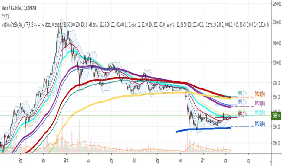
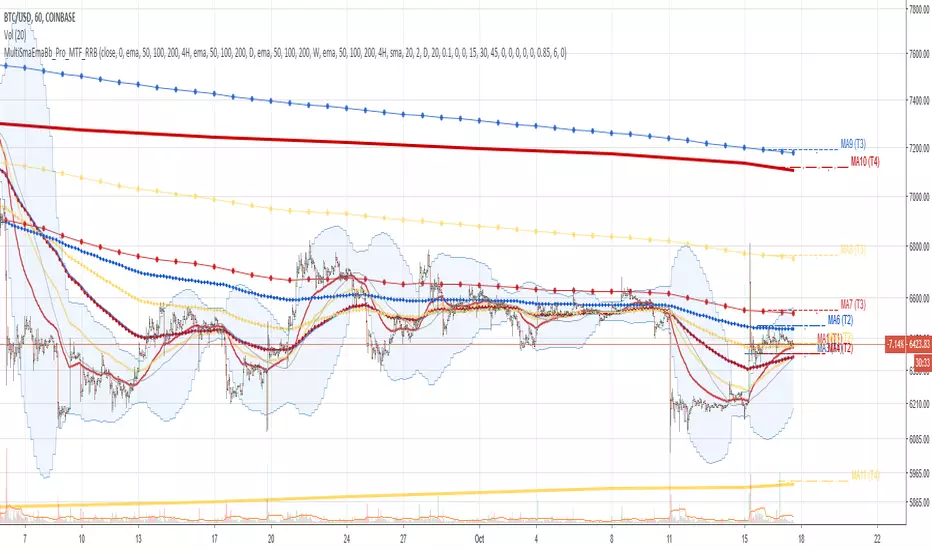
Multi SMA EMA WMA HMA BB (5x8 MAs Bollinger Bands) MAX MTF - RRBMulti SMA EMA WMA HMA 4x7 Moving Averages with Bollinger Bands MAX MTF by RagingRocketBull 2019
Version 1.0
All available MAX MTF versions are listed below (They are very similar and I don't want to publish them as separate indicators):
ver 1.0: 4x7 = 28 MTF MAs + 28 Levels + 3 BB = 59 < 64
ver 2.0: 5x6 = 30 MTF MAs + 30 Levels + 3 BB = 63 < 64
ver 3.0: 3x10 = 30 MTF MAs + 30 Levels + 3 BB = 63 < 64
ver 4.0: 5(4+1)x8 = 8 CurTF MAs + 32 MTF MAs + 20 Levels + 3 BB = 63 < 64
ver 5.0: 6(5+1)x6 = 6 CurTF MAs + 30 MTF MAs + 24 Levels + 3 BB = 63 < 64
ver 6.0: 4(3+1)x10 = 10 CurTF MAs + 30 MTF MAs + 20 Levels + 3 BB = 63 < 64
Fib numbers: 8, 13, 21, 34, 55, 89, 144, 233, 377
This indicator shows multiple MAs of any type SMA EMA WMA HMA etc with BB and MTF support, can show MAs as dynamically moving levels.
There are 4 MA groups + 1 BB group, a total of 4 TFs * 7 MAs = 28 MAs. You can assign any type/timeframe combo to a group, for example:
- EMAs 9,12,26,50,100,200,400 x H1, H4, D1, W1 (4 TFs x 7 MAs x 1 type)
- EMAs 8,13,21,30,34,50,55,89,100,144,200,233,377,400 x M15, H1 (2 TFs x 14 MAs x 1 type)
- D1 EMAs and SMAs 8,13,21,30,34,50,55,89,100,144,200,233,377,400 (1 TF x 14 MAs x 2 types)
- H1 WMAs 13,21,34,55,89,144,233; H4 HMAs 9,12,26,50,100,200,400; D1 EMAs 12,26,89,144,169,233,377; W1 SMAs 9,12,26,50,100,200,400 (4 TFs x 7 MAs x 4 types)
- +1 extra MA type/timeframe for BB
There are several versions: Simple, MTF, Pro MTF, Advanced MTF, MAX MTF and Ultimate MTF. This is the MAX MTF version. The Differences are listed below. All versions have BB
- Simple: you have 2 groups of MAs that can be assigned any type (5+5)
- MTF: +2 custom Timeframes for each group (2x5 MTF) +1 TF for BB, TF XY smoothing
- Pro MTF: 4 custom Timeframes for each group (4x3 MTF), 1 TF for BB, MA levels and show max bars back options
- Advanced MTF: +4 extra MAs/group (4x7 MTF), custom Ticker/Symbols, Timeframe <>= filter, Remove Duplicates Option
- MAX MTF: +2 subtypes/group, packed to the limit with max possible MAs/TFs: 4x7, 5x6, 3x10, 4(3+1)x10, 5(4+1)x8, 6(5+1)x6
- Ultimate MTF: +individual settings for each MA, custom Ticker/Symbols
MAX MTF version tests the limits of Pinescript trying to squeeze as many MAs/TFs as possible into a single indicator.
It's basically a maxed out Advanced version with subtypes allowing for mixed types within a group (i.e. both emas and smas in a single group/TF)
Pinescript has the following limits:
- max 40 security calls (6 calls are reserved for dupe checks and smoothing, 2 are used for BB, so only 32 calls are available)
- max 64 plot outputs (BB uses 3 outputs, so only 61 plot outputs are available)
- max 50000 (50kb) size of the compiled code
Based on those limits, you can only have the following MAs/TFs combos in a single script:
1. 4x7, 5x6, 3x10 - total number of MTF MAs must always be <= 32, and you can still have BB and Num Levels = total MAs, without any compromises
2. 5(4+1)x8, 6(5+1)x6, 4(3+1)x10 - you can use the Current Symbol/Timeframe as an extra (+1) fixed TF with the same number of MTF MAs
- you don't need to call security to display MAs on the Current Symbol/Timeframe, so the total number of MTF MAs remains the same and is still <= 32
- to fit that many MAs into the max 64 plot outputs limit you need to reduce the number of levels (not every MA Group will have corresponding levels)
Features:
- 4x7 = 28 MAs of any type
- 4x MTF groups with XY step line smoothing
- +1 extra TF/type for BB MAs
- 2 MA subtypes within each group/TF
- 4x7 = 28 MA levels with adjustable group offsets, indents and shift
- supports any existing type of MA: SMA, EMA, WMA, Hull Moving Average (HMA)
- custom tickers/symbols for each group
- show max bars back option
- show/hide both groups of MAs/levels/BB and individual MAs
- timeframe filter: show only MAs/Levels with TFs <>= Current TF
- hide MAs/Levels with duplicate TFs
- support for custom TFs that are not available in free accounts: 2D, 3D etc
- support for timeframes in H: H, 2H, 4H etc
Notes:
- Uses timeframe textbox instead of input resolution dropdown to allow for 240 120 and other custom TFs
- Uses symbol textbox instead of input symbol to avoid establishing multiple dummy security connections to the current ticker - otherwise empty symbols will prevent script from running
- Possible reasons for missing MAs on a chart:
- there may not be enough bars in history to start plotting it. For example, W1 EMA200 needs at least 200 bars on a weekly chart.
- for charts with low/fractional prices i.e. 0.00002 << 0.001 (default Y smoothing step) decrease Y smoothing as needed (set Y = 0.0000001) or disable it completely (set X,Y to 0,0)
- for charts with high price values i.e. 20000 >> 0.001 increase Y smoothing as needed (set Y = 10-20). Higher values exceeding MAs point density will cause it to disappear as there will be no points to plot. Different TFs may require diff adjustments
- TradingView Replay Mode UI and Pinescript security calls are limited to TFs >= D (D,2D,W,MN...) for free accounts
- attempting to plot any TF < D1 in Replay Mode will only result in straight lines, but all TFs will work properly in history and real-time modes. This is not a bug.
- Max Bars Back (num_bars) is limited to 5000 for free accounts (10000 for paid), will show error when exceeded. To plot on all available history set to 0 (default)
- Slow load/redraw times. This indicator becomes slower, its UI less responsive when:
- Pinescript Node.js graphics library is too slow and inefficient at plotting bars/objects in a browser window. Code optimization doesn't help much - the graphics engine is the main reason for general slowness.
- the chart has a long history (10000+ bars) in a browser's cache (you have scrolled back a couple of screens in a max zoom mode).
- Reload the page/Load a fresh chart and then apply the indicator or
- Switch to another Timeframe (old TF history will still remain in cache and that TF will be slow)
- in max possible zoom mode around 4500 bars can fit on 1 screen - this also slows down responsiveness. Reset Zoom level
- initial load and redraw times after a param change in UI also depend on TF. For example: D1/W1 - 2 sec, H1/H4 - 5-6 sec, M30 - 10 sec, M15/M5 - 4 sec, M1 - 5 sec. M30 usually has the longest history (up to 16000 bars) and W1 - the shortest (1000 bars).
- when indicator uses more MAs (plots) and timeframes it will redraw slower. Seems that up to 5 Timeframes is acceptable, but 6+ Timeframes can become very slow.
- show_last=last_bars plot limit doesn't affect load/redraw times, so it was removed from MA plot
- Max Bars Back (num_bars) default/custom set UI value doesn't seem to affect load/redraw times
- In max zoom mode all dynamic levels disappear (they behave like text)
- Dupe check includes symbol: symbol, tf, both subtypes - all must match for a duplicate group
- For the dupe check to work correctly a custom symbol must always include an exchange prefix. BB is not checked for dupes
Good Luck! Feel free to learn from/reuse the code to build your own indicators.

Multi SMA EMA WMA HMA BB (4x5 MAs Bollinger Bands) Adv MTF - RRBMulti SMA EMA WMA HMA 4x5 Moving Averages with Bollinger Bands Advanced MTF by RagingRocketBull 2019
Version 1.0
This indicator shows multiple MAs of any type SMA EMA WMA HMA etc with BB and MTF support, can show MAs as dynamically moving levels.
There are 4 MA groups + 1 BB group, a total of 4 TFs * 5 MAs = 20 MAs. You can assign any type/timeframe combo to a group, for example:
- EMAs 12,26,50,100,200 x H1, H4, D1, W1 (4 TFs x 5 MAs x 1 type)
- EMAs 8,10,13,21,30,50,55,100,200,400 x M15, H1 (2 TFs x 10 MAs x 1 type)
- D1 EMAs and SMAs 8,10,12,26,30,50,55,100,200,400 (1 TF x 10 MAs x 2 types)
- H1 WMAs 7,77,89,167,231; H4 HMAs 12,26,50,100,200; D1 EMAs 89,144,169,233,377; W1 SMAs 12,26,50,100,200 (4 TFs x 5 MAs x 4 types)
- +1 extra MA type/timeframe for BB
There are several versions: Simple, MTF, Pro MTF, Advanced MTF and Ultimate MTF. This is the Advanced MTF version. The Differences are listed below. All versions have BB
- Simple: you have 2 groups of MAs that can be assigned any type (5+5)
- MTF: +2 custom Timeframes for each group (2x5 MTF) +1 TF for BB, TF XY smoothing
- Pro MTF: 4 custom Timeframes for each group (4x3 MTF), 1 TF for BB, MA levels and show max bars back options
- Advanced MTF: +2 extra MAs/group (4x5 MTF), custom Ticker/Symbols, Timeframe <>= filter, Remove Duplicates Option
- Ultimate MTF: +individual settings for each MA, custom Ticker/Symbols
Features:
- 4x5 = 20 MAs of any type
- 4x MTF groups with XY step line smoothing
- +1 extra TF/type for BB MAs
- 4x5 = 20 MA levels with adjustable group offsets, indents and shift
- supports any existing type of MA: SMA, EMA, WMA, Hull Moving Average (HMA)
- custom tickers/symbols for each group - you can compare MAs of the same symbol across exchanges
- show max bars back option
- show/hide both groups of MAs/levels/BB and individual MAs
- timeframe filter: show only MAs/Levels with TFs <>= Current TF
- hide MAs/Levels with duplicate TFs
- support for custom TFs that are not available in free accounts: 2D, 3D etc
- support for timeframes in H: H, 2H, 4H etc
Notes:
- Uses timeframe textbox instead of input resolution dropdown to allow for 240 120 and other custom TFs
- Uses symbol textbox instead of input symbol to avoid establishing multiple dummy security connections to the current ticker - otherwise empty symbols will prevent script from running
- Possible reasons for missing MAs on a chart:
- there may not be enough bars in history to start plotting it. For example, W1 EMA200 needs at least 200 bars on a weekly chart.
- price << default Y smoothing step 5. For charts with low/fractional prices (i.e. 0.00002 << 5) adjust X Y smoothing as needed (set Y = 0.0000001) or disable it completely (set X,Y to 0,0)
- TradingView Replay Mode UI and Pinescript security calls are limited to TFs >= D (D,2D,W,MN...) for free accounts
- attempting to plot any TF < D1 in Replay Mode will only result in straight lines, but all TFs will work properly in history and real-time modes. This is not a bug.
- Max Bars Back (num_bars) is limited to 5000 for free accounts (10000 for paid), will show error when exceeded. To plot on all available history set to 0 (default)
- Slow load/redraw times. This indicator becomes slower, its UI less responsive when:
- Pinescript Node.js graphics library is too slow and inefficient at plotting bars/objects in a browser window. Code optimization doesn't help much - the graphics engine is the main reason for general slowness.
- the chart has a long history (10000+ bars) in a browser's cache (you have scrolled back a couple of screens in a max zoom mode).
- Reload the page/Load a fresh chart and then apply the indicator or
- Switch to another Timeframe (old TF history will still remain in cache and that TF will be slow)
- in max possible zoom mode around 4500 bars can fit on 1 screen - this also slows down responsiveness. Reset Zoom level
- initial load and redraw times after a param change in UI also depend on TF. For example:
D1/W1 - 2 sec, H1/H4 - 5-6 sec, M30 - 10 sec, M15/M5 - 4 sec, M1 - 5 sec.
M30 usually has the longest history (up to 16000 bars) and W1 - the shortest (1000 bars).
- when indicator uses more MAs (plots) and timeframes it will redraw slower. Seems that up to 5 Timeframes is acceptable, but 6+ Timeframes can become very slow.
- show_last=last_bars plot limit doesn't affect load/redraw times, so it was removed from MA plot
- Max Bars Back (num_bars) default/custom set UI value doesn't seem to affect load/redraw times
- In max zoom mode all dynamic levels disappear (they behave like text)
1. based on 3EmaBB, uses plot*, barssince and security functions
2. you can't set certain constants from input due to Pinescript limitations - change the code as needed, recompile and use as a private version
3. Levels = trackprice implementation
4. Show Max Bars Back = show_last implementation
5. swma has a fixed length = 4, alma and linreg have additional offset and smoothing params
6. Smoothing is applied by default for visual aesthetics on MTF. To use exact ma mtf values (lines with stair stepping) - disable it
Good Luck! You can explore, modify/reuse the code to build your own indicators.
Multi SMA EMA WMA HMA BB (4x3 MAs Bollinger Bands) Pro MTF - RRBMulti SMA EMA WMA HMA 4x3 Moving Averages with Bollinger Bands Pro MTF by RagingRocketBull 2018
Version 1.0
This indicator shows multiple MAs of any type SMA EMA WMA HMA etc with BB and MTF support, can show MAs as dynamically moving levels.
There are 4 MA groups + 1 BB group. You can assign any type/timeframe combo to a group, for example:
- EMAs 50,100,200 x H1, H4, D1, W1 (4 TFs x 3 MAs x 1 type)
- EMAs 8,13,21,55,100,200 x M15, H1 (2 TFs x 6 MAs x 1 type)
- D1 EMAs and SMAs 12,26,50,100,200,400 (1 TF x 6 MAs x 2 types)
- H1 WMAs 7,77,231; H4 HMAs 50,100,200; D1 EMAs 144,169,233; W1 SMAs 50,100,200 (4 TFs x 3 MAs x 4 types)
- +1 extra MA type/timeframe for BB
compile time: 25-30 sec
full redraw time after parameter change in UI: 3 sec
There are several versions: Simple, MTF, Pro MTF, Advanced MTF and Ultimate MTF. This is the Pro MTF version. The Differences are listed below. All versions have BB
- Simple: you have 2 groups of MAs that can be assigned any type (5+5)
- MTF: +2 custom Timeframes for each group (2x5 MTF)
- Pro MTF: +4 custom Timeframes for each group (4x3 MTF), MA levels and show max bars back options
- Advanced MTF: +2 extra MAs/group (4x5 MTF), custom Ticker/Symbol, backreferences for type, TF and MA lengths in UI
- Ultimate MTF: +individual settings for each MA, custom Ticker/Symbols
Features:
- 4x3 = 12 MAs of any type including Hull Moving Average (HMA)
- 4x MTF groups with step line smoothing
- BB +1 extra TF/type for BB MAs
- 12 MA levels with adjustable group offsets, indents and shift
- show max bars back
- you can show/hide both groups of MAs/levels and individual MAs
Notes:
1. based on 3EmaBB, uses plot*, barssince and security functions
2. you can't set certain constants from input due to Pinescript limitations - change the code as needed, recompile and use as a private version
3. Levels = trackprice implementation
4. Show Max Bars Back = show_last implementation
5. uses timeframe textbox instead of input resolution to allow for 120 240 and other custom TFs. Also supports TFs in hours: 2H or H2
6. swma has a fixed length = 4, alma and linreg have additional offset and smoothing params
7. Smoothing is applied by default for visual aesthetics on MTF. To use exact ma mtf values (lines with stair stepping) - disable it
MTF Notes:
- uses simple timeframe textbox instead of input resolution dropdown to allow for 120, 240 and other custom TFs, also supports timeframes in H: 2H, H2
- Groups that are not assigned a Custom TF will use Current Timeframe (0).
- MTF will work for any MA type assigned to the group
- MTF works both ways: you can display a higher TF MA/BB on a lower TF or a lower TF MA/BB on a higher TF.
- MTF MA values are normally aligned at the boundary of their native timeframe. This produces stair stepping when a higher TF MA is viewed on a lower TF.
Therefore X Y Point Density/Smoothing is applied by default on MA MTF for visual aesthetics. Set both to 0 to disable and see exact ma mtf values (lines with stair stepping and original mtf alignment).
- Smoothing is disabled for BB MTF bands because fill doesn't work with smoothed MAs after duplicate values are replaced with na.
- MTF MA Value fluctuation is possible on the current bar due to default security lookahead
Smoothing:
- X,Y == 0 - X,Y smoothing disabled (stair stepping on high TFs)
- X == 0, Y > 0 - X,Y smoothing applied to all TFs
- Y == 0, X > 0 - X smoothing applied to all TFs < deltaX_max_tf, Y smoothing disabled
- X > 0, Y > 0 - Y smoothing applied to all TFs, then X smoothing applied to all TFs < deltaX_max_tf
X Smoothing with Y == 0 - shows only every deltaX-th point starting from the first bar.
X Smoothing with Y > 0 - shows only every deltaX-th point starting from the last shown Y point, essentially filling huge gaps remaining after Y Smoothing with points and preserving the curve's general shape
X Smoothing on high TFs with already scarce points produces weird curve shapes, it works best only on high density lower TFs
Y Smoothing reduces points on all TFs, removes adjacent points with prices within deltaY, while preserving the smaller curve details.
A combination of X,Y produces the most accurate smoothing. Higher delta value - larger range, more points removed.
Show Max Bars Back:
- can't set plot show_last from input -> implemented using a timenow based range check
- you can't delete/modify history once plotted, so essentially it just sets a start point for plotting (from num_bars bars back) that works only in realtime mode (not in replay)
Levels:
You can plot current MA value using plot trackprice=true or by checking Show Price Line in Style. Problem is:
- you can only change color (not the dashed line style, width), have both ma + price line (not just the line), and it's full screen wide
- you can't set plot trackprice from input => implemented using plotshape/plotchar with fixed text labels serving as levels
- there's no other way of creating a dynamic level: hline, plot, offset - nothing else works.
- you can't plot a text var - all text strings must be constants, so you can't change the style, width and text labels without recompiling.
- from input you can only adjust offset, indent and shift for each level group, and change color
- the dot below each level line is the exact MA value. If you want just the line swap plotshape with plotchar, recompile and save as your private version, adjust Y shift.
To speed up redraw times: reduce last_bars to ~2000, recompile and use as your own private version
Pinescript is a rudimentary language (should be called Painscript instead) that can basically only plot data. You can't do much else. Please see the code for tips and hints.
Certain things just can't be done or require shady workarounds and weeks of testing trying to resolve weird node.js compiler errors.
Feel free to learn from/reuse/change the code as needed and use as your own private version. See comments in code. Good Luck!
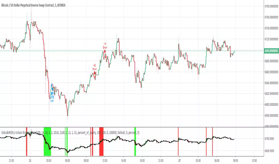
Gidra's Vchain Strategy v0.1Tested on "BTC/USD", this is a reversible strategy
If the RSI is lower than "RSI Limit" (for last "RSI Signals" candles) and there were "Open Color, Bars" green Heiken Ashi candles - close short, open long
If the RSI is higher than 100-"RSI Limit" (for last "RSI Signals" candles) and there were "Open Color, Bars" red Heiken Ashi candles - close long, open short
- timeframe: 5m (the best)
RSI Period = 14
RSI Limit = 30
RSI Signals = 3
Open Color = 2
Piramiding = 100
Lot = 100 %
- timeframe: 1h
RSI Period = 2
RSI Limit = 30
RSI Signals = 3
Open Color = 2
Piramiding = 100
Lot = 100 %
Fear–Greed Index📈 Fear–Greed Index
This indicator provides a sophisticated, multi-faceted measure of market sentiment, plotting it as an oscillator that ranges from -100 (Extreme Fear) to +100 (Extreme Greed).
Unlike standard indicators like RSI or MACD, this tool is built on principles from behavioral finance and social physics to model the complex psychology of the market. It does not use any of TradingView's built-in math functions and instead calculates everything from scratch.
🤔 How It Works: The Three-Model Approach
The final index is a comprehensive blend of three different academic models, each calculated across three distinct time horizons (Short, Mid, and Long) to capture sentiment at different scales.
Prospect Theory (CPT): This model, based on Nobel Prize-winning work, evaluates how traders perceive gains and losses. It assumes that the pain of a loss is felt more strongly than the pleasure of an equal gain, modeling the market's asymmetric emotional response.
Herding (Brock–Durlauf): This component measures the "follow the crowd" instinct. It analyzes the synchronization of positive and negative returns to determine if traders are acting in a coordinated, "herd-like" manner, which is a classic sign of building fear or greed.
Social Impact Theory (SIT): This model assesses how social forces influence market participants.
It combines three factors:
Strength (S): The magnitude of recent price moves (volatility).
Immediacy (I): How recently the most significant price action occurred.
Number (N): The level of market participation (volume).
The indicator calculates all three models for a Short, Mid, and Long lookback period. It then aggregates these nine components (3 models x 3 timeframes) using customizable weights to produce a single, final Fear–Greed Index value.
Interpretar How to Read the Index
Main Line: This is the final FGI score.
Lime/Green: Indicates Greed (positive values).
Red: Indicates Fear (negative values).
Fading Color: The color becomes more transparent as the index approaches the '0' (Neutral) line, and more solid as it moves toward the extremes.
Key Zones:
+100 to +30 (Extreme Greed): The market is highly euphoric and potentially overbought. This can be a contrarian signal for caution or profit-taking.
+30 to +18 (Greed Zone): Strong bullish sentiment.
+18 to -18 (Neutral Zone): The market is undecided, or fear and greed are in balance.
-18 to -30 (Fear Zone): Strong bearish sentiment.
-30 to -100 (Extreme Fear): The market is in a state of panic and may be oversold. This can be a contrarian signal for potential buying opportunities.
Reference Plots: The indicator also plots the aggregated scores for each of the three models (Herding, Prospect, and SIT) as faint, secondary lines. This allows you to see which component is driving the overall sentiment.
⚙️ Settings & Customization
This indicator is highly tunable, allowing you to adjust its sensitivity and component makeup.
Time Windows:
Short window: Lookback period for short-term sentiment.
Mid window: Lookback for medium-term sentiment.
Long window: Lookback for long-term sentiment.
Model Aggregation Weights:
Weight CPT, Weight Herding, Weight SIT: Control how much each of the three behavioral models contributes to the final score (they should sum to 1.0).
Cross-Horizon Weights:
Weight Short, Weight Mid, Weight Long: Control the influence of each timeframe on the final score (they should also sum to 1.0).
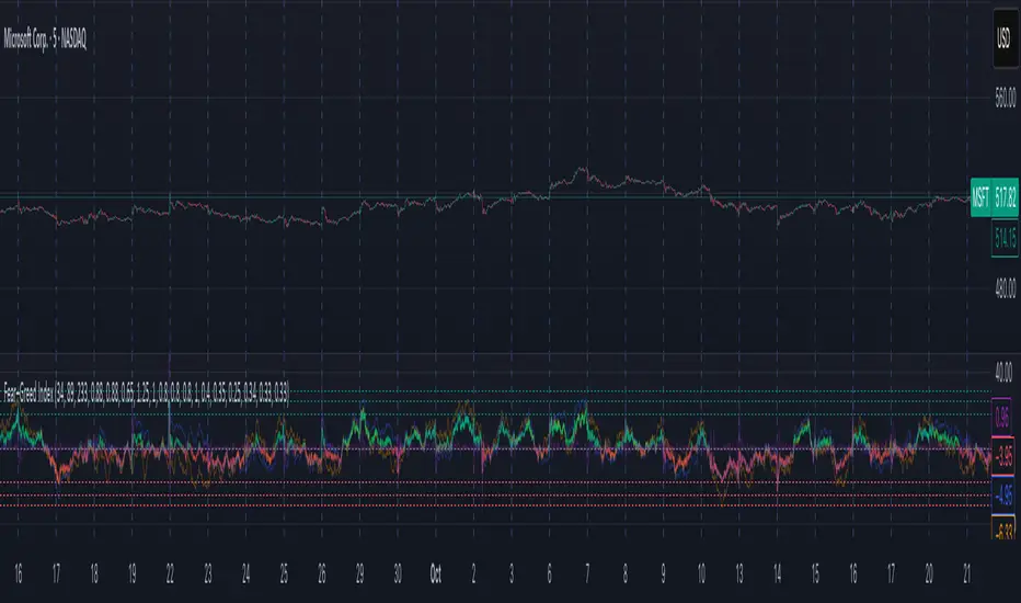
EMA100 Breakout by shubhThis indicator is a clean, price-action-based breakout system designed for disciplined trend trading on any timeframe — especially for Nifty and Bank Nifty spot, futures, and options charts.
It uses a single 100-period EMA to define trend direction and waits for decisive candle closes across the EMA to trigger potential entries.
The logic ensures only one active trade at a time, enforcing patience and clarity in decision-making.
⚙️ Core Logic
Buy Setup
A bullish candle closes above the 100 EMA while its open was below the EMA.
Entry occurs at candle close.
Stop-Loss (SL): Low of the signal candle.
Target (TP): 4 × the SL distance (Risk : Reward = 1 : 4).
Sell Setup
A bearish candle closes below the 100 EMA while its open was above the EMA.
Entry occurs at candle close.
Stop-Loss (SL): High of the signal candle.
Target (TP): 4 × the SL distance.
Trade Management
Only one trade may run at a time (either long or short).
New signals are ignored until the current position hits SL or TP.
Transparent labels show Entry, SL, and TP levels on chart.
Dotted lines visualize active Stop-Loss (red) and Target (green).
Exit markers:
✅ Target Hit
❌ Stop Loss Hit
🧠 Key Advantages
Simple and transparent trend-following logic.
Enforces disciplined “one-trade-at-a-time” behavior.
High risk-to-reward (1 : 4).
Works across timeframes — 5 min to Daily.
Ideal for intraday and positional setups.
📊 Suggested Use
Apply on Nifty / Bank Nifty spot or futures charts.
Works on any instrument with clear momentum swings.
Best confirmation when EMA 100 acts as dynamic support/resistance.
⚠️ Disclaimer
This script is for educational and research purposes only.
It is not financial advice or an invitation to trade.
Always backtest thoroughly and manage risk responsibly before applying in live markets.
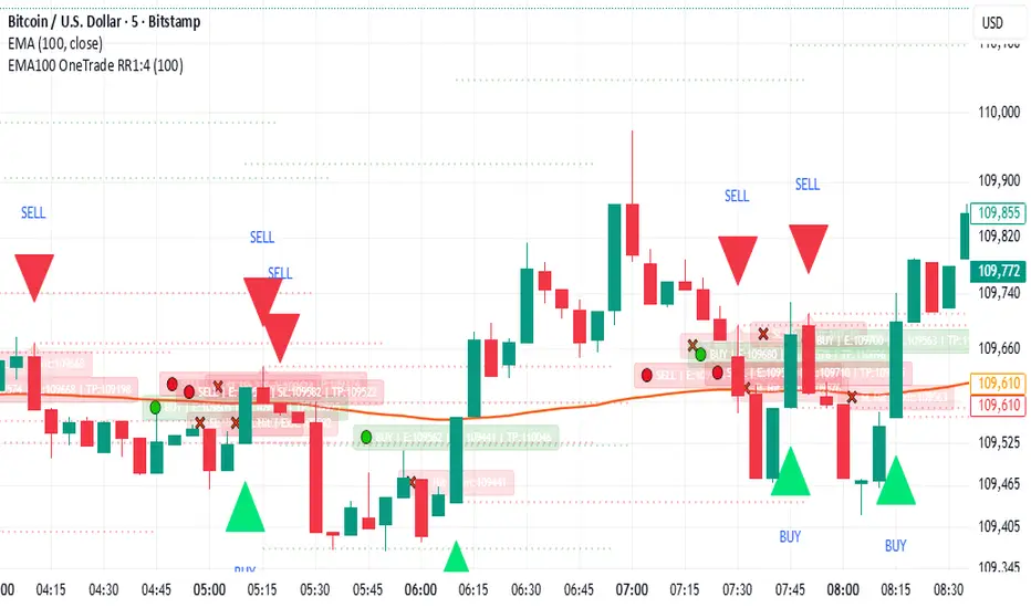
RRG Sector Snapshot RRG Sector Snapshot · Clear UI — User Guide
What this indicator does
Purpose: Visualize sector rotation by comparing each sector’s Relative Strength (RS-Ratio) and RS-Momentum versus a benchmark (e.g., VNINDEX).
Output: A quadrant map (table overlay) that positions each sector into one of four regimes:
LEADING (top-right): Strong and accelerating — leadership zone.
WEAKENING (bottom-right): Strong but decelerating — may be topping or consolidating.
LAGGING (bottom-left): Weak and decelerating — avoid unless mean-reverting.
IMPROVING (top-left): Weak but accelerating — candidates for next rotation into leadership.
How it works (under the hood)
X-axis (Strength): RS-Ratio = Sector Close / Benchmark Close, then normalized with a Z-Score over a lookback (normLen).
Y-axis (Momentum): Linear-regression slope of RS-Ratio over rsLen, then normalized with a Z-Score (normLen).
Mapping to grid: Both axes are Z-Scores scaled to a square grid (rrgSize × rrgSize) using a zoom factor (rrgScale). The center is neutral (0,0). Momentum increases upward (Y=0 is the top row in the table).
Quick start (3 minutes)
Add to chart:
TradingView → Pine Editor → paste the script → Save → Add to chart.
Set a benchmark: In inputs, choose Benchmark (X axis) — default INDEX:VNINDEX. Use VN30 or another index if it better reflects your universe.
Load sectors: Fill S1..S10 with sector or index symbols you track (up to 10). Set Slots to Use to the number you actually use.
Adjust view:
rrgSize (grid cells): 18–24 is a good starting point.
rrgScale (zoom): 2.5–3.5 typically; decrease to “zoom out” (points cluster near center), increase to “zoom in” (points spread to edges).
Read the map:
Prioritize sectors in LEADING; shortlist sectors in IMPROVING (could rotate into LEADING).
WEAKENING often marks late-cycle strength; LAGGING is typically avoid.
Inputs — what they do and how to change them
General
Analysis TF: Timeframe used to compute RRG (can be different from chart’s TF). Daily for swing, 1H/4H for tactical rotation, Weekly for macro view.
Benchmark (X axis): The index used for RS baseline (e.g., INDEX:VNINDEX, INDEX:VN30, major ETFs, or a custom composite).
RRG Calculation
RS Lookback (rsLen): Bars used for slope of RS (momentum).
Daily: 30–60 (default 40)
Intraday (1H/4H): 20–40
Weekly: 26–52
Normalization Lookback (Z-Score) (normLen): Window for Z-Score on both axes.
Daily: 80–120 (default 100)
Intraday: 40–80
Weekly: 52–104
Tip: Shorter lookbacks = more responsive but noisier; longer = smoother but slower.
RRG HUD (Table)
Show RRG Snapshot (rrgEnable): Toggle the table on/off.
Position (rrgPos): top_right | top_left | bottom_right | bottom_left.
Grid Size (Cells) (rrgSize): Table dimensions (N×N). Larger = more resolution but takes more space.
Z-Scale (Zoom) (rrgScale): Maps Z-Scores to the grid.
Smaller (2.0–2.5): Zoom out (more points near center).
Larger (3.5–4.0): Zoom in (emphasize outliers).
Appearance
Tag length (tagLen): Characters per sector tag. Use 4–6 for clarity.
Text size (textSizeOp): Tiny | Small | Normal | Large. Use Large for presentation screens or dense lists.
Axis thickness (axisThick): 1 = thin axis; 2 = thicker double-strip axis.
Quadrant alpha (bgAlpha): Transparency of quadrant backgrounds. 80–90 makes text pop.
Sectors (Max 10)
Slots to Use (sectorSlots): How many sector slots are active (≤10).
S1..S10: Each slot is a symbol (index, sector index, or ETF). Replace defaults to fit your market/universe.
How to interpret the map
Quadrants:
Leading (top-right): Relative strength above average and improving — trend-follow candidates.
Weakening (bottom-right): Still strong but momentum cooling — watch for distribution or pauses.
Lagging (bottom-left): Underperforming and still losing momentum — avoid unless doing mean-reversion.
Improving (top-left): Early recovery — candidates to transition into Leading if the move persists.
Overlapping sectors in one cell: The indicator shows “TAG +n” where TAG is the first tag, +n is the number of additional sectors sharing that cell. If many overlap:
Increase rrgSize, or
Decrease rrgScale to zoom out, or
Reduce Slots to Use to a smaller selection.
Suggested workflows
Daily swing
Benchmark: VNINDEX or VN30
rsLen 40–60, normLen 100–120, rrgSize 18–24, rrgScale 2.5–3.5
Routine:
Identify Leading sectors (top-right).
Spot Improving sectors near the midline moving toward top-right.
Confirm with price/volume/breakout on sector charts or top components.
Intraday (1H/4H) tactical
rsLen 20–40, normLen 60–100, rrgScale 2.0–3.0
Expect faster rotations and more noise; tighten filters with your own entry rules.
Weekly (macro rotation)
rsLen 26–52, normLen 52–104, rrgScale 3.0–4.0
Great for portfolio tilts and sector allocation.
Tuning tips
If everything clusters near center: Increase rrgScale (zoom in) or reduce normLen (more contrast).
If points are too spread: Decrease rrgScale (zoom out) or increase normLen (smoother normalization).
If the table is too big/small: Change rrgSize (cells).
If tags are hard to read: Increase textSizeOp to Large, tagLen to 5–6, and consider bgAlpha ~80–85.
Troubleshooting
No table on chart:
Ensure Show RRG Snapshot is enabled.
Change Position to a different corner.
Reduce Grid Size if the table exceeds the chart area.
Many sectors “missing”:
They’re likely overlapping in the same cell; the cell will show “TAG +n”.
Increase rrgSize, decrease rrgScale, or reduce Slots to Use.
Early bars show nothing:
You need enough data for rsLen and normLen. Scroll back or reduce lookbacks temporarily.
Best practices
Use RRG for context and rotation scouting, then confirm with your execution tools (trend structure, breakouts, volume, risk metrics).
Benchmark selection matters. If most of your watchlist tracks VN30, use INDEX:VN30 as the benchmark to get a truer relative read.
Revisit settings per timeframe. Intraday needs more responsiveness (shorter lookbacks, smaller Z-Scale); weekly needs stability (longer lookbacks, larger Z-Scale).
FAQ
Can I use ETFs or custom indices as sectors? Yes. Any symbol supported by TradingView works.
Can I track individual stocks instead of sectors? Yes (up to 10); just replace the S1..S10 symbols.
Why Z-Score? It standardizes each axis to “how unusual” the value is versus its own history — more robust than raw ratios across different scales.
[ i]
How to Set Up (Your Market Template)
This is the most important part for customizing the indicator to any market.
Step 1: Choose Your TF & Benchmark
Open the indicator's Settings.
Analysis TF: Set the timeframe you want to analyze (e.g., D for medium-term, W for long-term).
Benchmark (Trục X): This is the index you want to compare against.
Vietnamese Market: Leave the default INDEX:VNINDEX.
US Market: Change to SP:SPX or NASDAQ:NDX.
Crypto Market: Change to TOTAL (entire market cap) or BTC.D (Bitcoin Dominance).
Step 2: Input Your "Universe" (The 10 Slots)
This is where you decide what to track. You have 10 slots (S1 to S10).
For Vietnamese Sectors (Default):
Leave the default sector codes like INDEX:VNFINLEAD (Finance), INDEX:VNREAL (Real Estate), INDEX:VNIND (Industry), etc.
Template for Crypto "Sectors":
S1: BTC.D
S2: ETH.D
S3: TOTAL2 (Altcoin Market Cap)
S4: TOTAL.DEFI (DeFi)
S5: CRYPTOCAP:GAME (GameFi)
...and so on.
Template for Blue Chip Stocks:
Benchmark: INDEX:VN30
S1: HOSE:FPT
S2: HOSE:VCB
S3: HOSE:HPG
S4: HOSE:MWG
...and so on.
Template for Commodities:
Benchmark: TVC:DXY (US Dollar Index)
S1: TVC:GOLD
S2: TVC:USOIL
S3: TVC:SILVER
S4: COMEX:HG1! (Copper)
...and so on.
Step 3: Fine-Tuning
RS Lookback: A larger number (e.g., 100) gives a smoother, long-term view. A smaller number (e.g., 20) is more sensitive to short-term changes.
Z-Scale (Zoom): This is the "magnification" of the map.
If all your sectors are crowded in the middle, increase this number (e.g., 4.0) to "zoom in."
If your sectors are stuck on the edges, decrease this number (e.g., 2.0) to "zoom out."
Tag length: How many letters to display for the ticker (e.g., 4 will show VNFI).

Lot Size Calculator - Gold🥇 Lot Size Calculator for Gold (XAU/USD)
Description:
A professional and accurate lot size calculator specifically designed for Gold (XAU/USD) trading. This indicator helps traders calculate the optimal position size based on account balance, risk percentage, and stop loss distance, ensuring proper risk management for every trade.
Key Features:
Accurate Gold Calculations - Properly accounts for Gold pip values ($10 per pip for standard 100oz lots)
Multi-Currency Support - Works with USD, EUR, and GBP account currencies
Flexible Contract Sizes - Supports Standard (100 oz), Mini (10 oz), and Micro (1 oz) lots
Customizable Decimal Places - Display lot sizes with 2-8 decimal precision (no rounding)
Clean Visual Design - Modern, professional info panel with gold-themed styling
Adjustable Display - Position panel anywhere on chart with customizable colors and sizes
Real-Time Calculations - Instantly updates as you adjust your risk parameters
How It Works:
The calculator uses the standard forex position sizing formula optimized for Gold:
Lot Size = Risk Amount / (Stop Loss in Pips × Pip Value Per Lot)
For Gold (XAU/USD):
Standard Lot (100 oz): 1 pip = $10
Mini Lot (10 oz): 1 pip = $1
Micro Lot (1 oz): 1 pip = $0.10
Settings:
Account Settings:
Account Balance: Your trading capital
Account Currency: USD, EUR, or GBP
Risk Percentage: How much to risk per trade (default: 2%)
Contract Size: 100 oz (Standard), 10 oz (Mini), or 1 oz (Micro)
Display Currency: Choose how to display risk amounts
Trade Settings:
Stop Loss: Your SL distance in pips
Display Settings:
Label Position: Top/Bottom, Left/Right, Middle Right
Label Size: Tiny to Huge
Decimal Places: 2-8 decimals
Custom Colors: Background, text, and accent colors
Perfect For:
Gold (XAU/USD) day traders and swing traders
Position sizing and risk management
Traders using fixed percentage risk models
Anyone trading Gold CFDs or spot markets
Scalpers to long-term Gold investors
What Makes This Different:
Unlike generic lot size calculators, this tool correctly calculates Gold's pip values based on contract size. Many calculators get this wrong, leading to incorrect position sizing. This indicator ensures you're always trading the right lot size for your risk tolerance.
Example Usage:
Account Balance: $10,000
Risk: 1% = $100
Stop Loss: 60 pips
Contract Size: 100 oz (Standard)
Result: 0.1667 lots (exact, no rounding)
Perfect for maintaining consistent risk management in your Gold trading strategy!

Fixed High Timeframe Moving AveragesFixed High Timeframe Moving Averages (W/D/4H)
Summary
This indicator plots essential, high-timeframe (HTF) Moving Averages onto your chart, **no matter which timeframe you are currently viewing**.
It is designed for traders who need multi-timeframe context at a glance. Stop switching charts to see where the 200-Week or 50-Day MA is—now you can see all critical HTF levels directly on your 5-minute (or any other) chart.
---
Who it’s for
Traders who rely on moving averages but like to work on lower chart timeframes while keeping higher timeframe context in sight. If you scalp on 1–15m yet want Weekly/Daily/4H MAs always visible, this is for you.
---
What it shows
Pinned (“fixed”) moving averages from higher timeframes—Weekly (20/100/200) , Daily (50/100/200/365) and 4H (200) —rendered on any chart timeframe. Your favorite HTF MAs stay on screen no matter what TF you’re currently analyzing.
---
Features
* **MA types:** SMA, EMA, VWMA, Hull.
* **Fully configurable:** toggle each line, set periods, colors, and thickness.
* **Two alert modes (see below):** intrabar vs confirmed HTF close.
* **Works on any symbol & chart TF** using `request.security` to fetch HTF data.
---
Alerts & Modes
This indicator solves the biggest problem with MTF alerts: false signals. You can choose one of two modes:
1. **Intrabar mode** — compares current chart price to the HTF MA. Triggers as soon as price crosses the HTF line; great for early signals but may update until the HTF bar closes.
2. **Confirmed mode** — checks HTF close vs HTF MA. Signals only on the higher-TF bar close; fewer false starts, no intrabar repainting on that TF.
Per-line *Cross Above / Cross Below* conditions are provided for all enabled MAs (e.g., “20W — Cross Above”, “365D — Cross Below”, etc.).
**How to use alerts:** add the script → “Create Alert” → pick any condition from the script’s list.
---
Why this helps
* Keeps Weekly/Daily structure visible while you execute on LTF.
* Classic anchors (e.g., 200D, 20W/100W/200W) are popular for trend bias, dynamic support/resistance, and pullback context.
* Lets you standardize MA references across all your lower-TF playbooks.
---
Notes on confirmation & repainting
* Intrabar signals can change until the higher-TF bar closes (that’s expected with multi-TF data).
* Confirmed mode waits for the HTF close—cleaner, but later. Choose what fits your workflow.
---
Quick setup
1. Pick `MA Type` (SMA/EMA/VWMA/Hull).
2. Enable the HTF lines you want (Weekly 20/100/200; Daily 50/100/200/365; 4H 200).
3. Choose `Alert Mode` (Intrabar vs Confirmed).
4. Style colors/widths to taste and set alerts on the lines you care about.
---
Good practice
* Combine HTF MAs with price action (swings, structure, liquidity grabs) rather than using them in isolation.
* Always validate signals in your execution TF and use a risk plan tailored to volatility.
* Protect your capital: position sizing, stops, and disciplined risk management matter more than any single line on the chart.
---
Disclaimer
For educational/informational purposes only; not financial advice. Trading involves risk—manage it responsibly.

Trend Catch STFR - whipsaw Reduced### Summary of the Setup
This trading system combines **SuperTrend** (a trend-following indicator based on ATR for dynamic support/resistance), **Range Filter** (a smoothed median of the last 100 candles to identify price position relative to a baseline), and filters using **VIX Proxy** (a volatility measure: (14-period ATR / 14-period SMA of Close) × 100) and **ADX** (Average Directional Index for trend strength). It's designed for trend trading with volatility safeguards.
- **Entries**: Triggered only in "tradeable" markets (VIX Proxy ≥ 15 OR ADX ≥ 20) when SuperTrend aligns with direction (green for long, red for short), price crosses the Range Filter median accordingly, and you're not already in that position.
- **Exits**: Purely price-based—exit when SuperTrend flips or price crosses back over the Range Filter median. No forced exits from low volatility/trend.
- **No Trade Zone**: Blocks new entries if both VIX Proxy < 15 AND ADX < 20, but doesn't affect open positions.
- **Overall Goal**: Enter trends with confirmed strength/volatility, ride them via price action, and avoid ranging/choppy markets for new trades.
This creates a filtered trend-following strategy that prioritizes quality entries while letting winners run.
### Advantages
- **Reduces Noise in Entries**: The VIX Proxy and ADX filters ensure trades only in volatile or strongly trending conditions, avoiding low-momentum periods that often lead to false signals.
- **Lets Winners Run**: Exits based solely on price reversal (SuperTrend or Range Filter) allow positions to stay open during temporary lulls in volatility/trend, potentially capturing longer moves.
- **Simple and Balanced**: Combines trend (SuperTrend/ADX), range (Filter), and volatility (VIX Proxy) without overcomplicating—easy to backtest and adapt to assets like stocks, forex, or crypto.
- **Adaptable to Markets**: The "OR" logic for VIX/ADX provides flexibility (e.g., enters volatile sideways markets if ADX is low, or steady trends if VIX is low).
- **Risk Control**: Implicitly limits exposure by blocking entries in calm markets, which can preserve capital during uncertainty.
### Disadvantages
- **Whipsaws in Choppy Markets**: As you noted, SuperTrend can flip frequently in ranging conditions, leading to quick entries/exits and small losses, especially if the Range Filter isn't smoothing enough noise.
- **Missed Opportunities**: Strict filters (e.g., requiring VIX ≥ 15 or ADX ≥ 20) might skip early-stage trends or low-volatility grinds, reducing trade frequency and potential profits in quiet bull/bear markets.
- **Lagging Exits**: Relying only on price flips means you might hold losing trades longer if volatility drops without a clear reversal, increasing drawdowns.
- **Parameter Sensitivity**: Values like VIX 15, ADX 20, or Range Filter's 100-candle lookback need tuning per asset/timeframe; poor choices could amplify whipsaws or over-filter.
- **No Built-in Risk Management**: Lacks explicit stops/targets, so it relies on user-added rules (e.g., ATR-based stops), which could lead to oversized losses if not implemented.
### How to Use It
This system can be implemented in platforms like TradingView (via Pine Script), Python (e.g., with TA-Lib or Pandas), or MT4/5. Here's a step-by-step guide, assuming TradingView for simplicity—adapt as needed. (If coding in Python, use libraries like pandas_ta for indicators.)
1. **Set Up Indicators**:
- Add SuperTrend (default: ATR period 10, multiplier 3—adjust as suggested in prior tweaks).
- Create Range Filter: Use a 100-period SMA of (high + low)/2, smoothed (e.g., via EMA if desired).
- Calculate VIX Proxy: Custom script for (ATR(14) / SMA(close, 14)) * 100.
- Add ADX (period 14, standard).
2. **Define Rules in Code/Script**:
- **Long Entry**: If SuperTrend direction < 0 (green), close > RangeFilterMedian, (VIX Proxy ≥ 15 OR ADX ≥ 20), and not already long—buy on bar close.
- **Short Entry**: If SuperTrend direction > 0 (red), close < RangeFilterMedian, (VIX Proxy ≥ 15 OR ADX ≥ 20), and not already short—sell short.
- **Exit Long**: If in long and (SuperTrend > 0 OR close < RangeFilterMedian)—sell.
- **Exit Short**: If in short and (SuperTrend < 0 OR close > RangeFilterMedian)—cover.
- Monitor No Trade Zone visually (e.g., plot yellow background when VIX < 15 AND ADX < 20).
3. **Backtest and Optimize**:
- Use historical data on your asset (e.g., SPY on 1H chart).
- Test metrics: Win rate, profit factor, max drawdown. Adjust thresholds (e.g., ADX to 25) to reduce whipsaws.
- Forward-test on demo account to validate.
4. **Live Trading**:
- Apply to a chart, set alerts for entries/exits.
- Add risk rules: Position size 1-2% of capital, stop-loss at SuperTrend line.
- Monitor manually or automate via bots—avoid overtrading; use on trending assets.
For the adjustments I suggested earlier (e.g., ADX 25, 2-bar confirmation), integrate them into entries only—test one at a time to isolate improvements. If whipsaws persist, combine 2-3 tweaks.

Mean Reversion Oscillator [Alpha Extract]An advanced composite oscillator system specifically designed to identify extreme market conditions and high-probability mean reversion opportunities, combining five proven oscillators into a single, powerful analytical framework.
By integrating multiple momentum and volume-based indicators with sophisticated extreme level detection, this oscillator provides precise entry signals for contrarian trading strategies while filtering out false reversals through momentum confirmation.
🔶 Multi-Oscillator Composite Framework
Utilizes a comprehensive approach that combines Bollinger %B, RSI, Stochastic, Money Flow Index, and Williams %R into a unified composite score. This multi-dimensional analysis ensures robust signal generation by capturing different aspects of market extremes and momentum shifts.
// Weighted composite (equal weights)
normalized_bb = bb_percent
normalized_rsi = rsi
normalized_stoch = stoch_d_val
normalized_mfi = mfi
normalized_williams = williams_r
composite_raw = (normalized_bb + normalized_rsi + normalized_stoch + normalized_mfi + normalized_williams) / 5
composite = ta.sma(composite_raw, composite_smooth)
🔶 Advanced Extreme Level Detection
Features a sophisticated dual-threshold system that distinguishes between moderate and extreme market conditions. This hierarchical approach allows traders to identify varying degrees of mean reversion potential, from moderate oversold/overbought conditions to extreme levels that demand immediate attention.
🔶 Momentum Confirmation System
Incorporates a specialized momentum histogram that confirms mean reversion signals by analyzing the rate of change in the composite oscillator. This prevents premature entries during strong trending conditions while highlighting genuine reversal opportunities.
// Oscillator momentum (rate of change)
osc_momentum = ta.mom(composite, 5)
histogram = osc_momentum
// Momentum confirmation
momentum_bullish = histogram > histogram
momentum_bearish = histogram < histogram
// Confirmed signals
confirmed_bullish = bullish_entry and momentum_bullish
confirmed_bearish = bearish_entry and momentum_bearish
🔶 Dynamic Visual Intelligence
The oscillator line adapts its color intensity based on proximity to extreme levels, providing instant visual feedback about market conditions. Background shading creates clear zones that highlight when markets enter moderate or extreme territories.
🔶 Intelligent Signal Generation
Generates precise entry signals only when the composite oscillator crosses extreme thresholds with momentum confirmation. This dual-confirmation approach significantly reduces false signals while maintaining sensitivity to genuine mean reversion opportunities.
How It Works
🔶 Composite Score Calculation
The indicator simultaneously tracks five different oscillators, each normalized to a 0-100 scale, then combines them into a smoothed composite score. This approach eliminates the noise inherent in single-oscillator analysis while capturing the consensus view of multiple momentum indicators.
// Mean reversion entry signals
bullish_entry = ta.crossover(composite, 100 - extreme_level) and composite < (100 - extreme_level)
bearish_entry = ta.crossunder(composite, extreme_level) and composite > extreme_level
// Bollinger %B calculation
bb_basis = ta.sma(src, bb_length)
bb_dev = bb_mult * ta.stdev(src, bb_length)
bb_percent = (src - bb_lower) / (bb_upper - bb_lower) * 100
🔶 Extreme Zone Identification
The system automatically identifies when markets reach statistically significant extreme levels, both moderate (65/35) and extreme (80/20). These zones represent areas where mean reversion has the highest probability of success based on historical market behavior.
🔶 Momentum Histogram Analysis
A specialized momentum histogram tracks the velocity of oscillator changes, helping traders distinguish between healthy corrections and potential trend reversals. The histogram's color-coded display makes momentum shifts immediately apparent.
🔶 Divergence Detection Framework
Built-in divergence analysis identifies situations where price and oscillator movements diverge, often signaling impending reversals. Diamond-shaped markers highlight these critical divergence patterns for enhanced pattern recognition.
🔶 Real-Time Information Dashboard
An integrated information table provides instant access to current oscillator readings, market status, and individual component values. This dashboard eliminates the need to manually check multiple indicators while trading.
🔶 Individual Component Display
Optional display of individual oscillator components allows traders to understand which specific indicators are driving the composite signal. This transparency enables more informed decision-making and deeper market analysis.
🔶 Adaptive Background Coloring
Intelligent background shading automatically adjusts based on market conditions, creating visual zones that correspond to different levels of mean reversion potential. The subtle color gradations make pattern recognition effortless.
1D
3D
🔶 Comprehensive Alert System
Multi-tier alert system covers confirmed entry signals, divergence patterns, and extreme level breaches. Each alert type provides specific context about the detected condition, enabling traders to respond appropriately to different signal strengths.
🔶 Customizable Threshold Management
Fully adjustable extreme and moderate levels allow traders to fine-tune the indicator's sensitivity to match different market volatilities and trading timeframes. This flexibility ensures optimal performance across various market conditions.
🔶 Why Choose AE - Mean Reversion Oscillator?
This indicator provides the most comprehensive approach to mean reversion trading by combining multiple proven oscillators with advanced confirmation mechanisms. By offering clear visual hierarchies for different extreme levels and requiring momentum confirmation for signals, it empowers traders to identify high-probability contrarian opportunities while avoiding false reversals. The sophisticated composite methodology ensures that signals are both statistically significant and practically actionable, making it an essential tool for traders focused on mean reversion strategies across all market conditions.
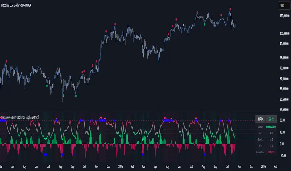
Volatility Channel Oscillator█ OVERVIEW
"Volatility Channel Oscillator" is a technical indicator that analyzes price volatility relative to dynamic price channels, displaying an oscillator, its moving average, and signals based on crossovers and divergences. The indicator offers customizable overbought and oversold levels, gradient visualization, and divergence detection, supported by alerts for key signals.
█ CONCEPTS
The VCO indicator creates dynamic price channels based on a moving average of the price (calculated as the arithmetic mean of the high and low prices: (high + low) / 2) and market volatility (measured as the average candle range and body size). These channels are not displayed on the chart but are used to calculate the oscillator value, which reflects the position of the closing price relative to the channel width, scaled to a range from -100 to +100, with the zero line as the central point. A moving average of the oscillator (SMA) smooths its values, enabling signals based on crossovers with the zero line or overbought/oversold levels. The indicator also detects divergences between price and the oscillator, which may indicate potential trend reversals. VCO is useful for identifying market momentum, reversal points, and trend confirmation, especially when combined with other technical analysis tools.
█ FEATURES
- Volatility Channels: Calculates invisible chart boundaries based on a simple moving average (SMA) of the price (high + low) / 2 and volatility (average candle range and body). The length parameter (default 30) sets the SMA length, and scale (default 200%) adjusts the channel width.
- Oscillator: Determines the oscillator value in the range of -100 to +100, indicating the closing price's position relative to the volatility channel. Displayed with dynamic coloring (green for positive values, red for negative).
- Oscillator Moving Average: A simple moving average (SMA) of the oscillator values, smoothing its movements. The signalLength parameter (default 20) defines the SMA length. Displayed in yellow with an optional gradient.
- Overbought/Oversold Levels: Configurable thresholds for the oscillator (overbought, default 50; oversold, default -50) and its moving average (maOverbought, default 30; maOversold, default -30), shown as horizontal lines with optional gradients. Band colors change dynamically (red for overbought, green for oversold, gray for neutral) based on the moving average's position relative to maOverbought/maOversold, reinforcing other signals.
- Divergences: Detects bullish (price forms a lower low, oscillator a higher low) and bearish (price forms a higher high, oscillator a lower high) divergences using pivots (pivotLength, default 2). Divergences are displayed with a delay equal to the pivot length; larger lengths increase reliability but delay signals. Use as additional confirmation.
Signals:
- Overbought/Oversold Crossovers: Green triangles (buy) when the oscillator crosses above the oversold level, red triangles (sell) when it crosses below the overbought level.
- Zero Line Crossovers: Buy/sell signals when the oscillator crosses the zero line upward (buy) or downward (sell).
- Moving Average Crossovers: Buy/sell signals when the oscillator's moving average crosses the zero line or the maOverbought/maOversold levels. Dynamic band color changes (red/green) at these crossovers reinforce other signals.
- Visualization: Gradient lines for the oscillator, its moving average, overbought/oversold levels, and zero line, with adjustable transparency. Gradient fill between the oscillator and zero line.
Divergence Labels: "Bull" (bullish) and "Bear" (bearish) labels with customizable color and transparency.
- Alerts: Built-in alerts for divergences, overbought/oversold crossovers, and zero line crossovers by the oscillator and its moving average.
█ HOW TO USE
Add to Chart: Apply the indicator via Pine Editor or the Indicators menu on TradingView.
Configure Settings:
- Channel and Oscillator Settings: Adjust the channel SMA length (length, default 30) and channel scaling (scale, default 200%). Increase scale for high-volatility markets.
- Threshold Levels: Set oscillator overbought (overbought, default 50) and oversold (oversold, default -50) levels, and moving average thresholds (maOverbought, default 30; maOversold, default -30).
- Divergence Settings: Enable/disable divergence detection (calculateDivergence) and set pivot length (pivotLength, default 2). Larger values increase reliability but delay signals.
- Signal Settings: Choose signal types (signalType): overbought/oversold, zero line, moving average, or all.
- Styling: Customize colors for the oscillator, moving average, horizontal levels, and divergence labels. Adjust gradient and fill transparency.
Interpreting Signals:
- Buy Signals: Green triangles below the bar when the oscillator or its moving average crosses above the oversold level or zero line.
- Sell Signals: Red triangles above the bar when the oscillator or its moving average crosses below the overbought level or zero line.
- Moving Average Signals: Green/red triangles when the moving average crosses maOverbought/maOversold levels, indicating potential reversals or trend continuation. Dynamic band color changes (red for overbought, green for oversold) at these crossovers reinforce other signals.
- Divergences: "Bull" (bullish) and "Bear" (bearish) labels indicate potential trend reversals with a delay based on pivot length. Use as confirmation.
- Overbought/Oversold Levels: Monitor price reactions in these zones as potential reversal points. Dynamic band color changes based on the moving average reinforce signals.
Signal Confirmation: Use VCO with other tools, such as pivot levels (for key turning points) or Fibonacci levels (for support/resistance zones).
█ APPLICATIONS
- Trend Trading: Zero line crossovers by the oscillator or its moving average identify momentum in uptrends or downtrends.
- Range Trading: Overbought/oversold levels help identify entry/exit points in sideways markets.
- Divergences: Use bullish/bearish divergences as additional confirmation of reversals, especially near key price levels.
- Trend Identification: To analyze trends over a longer perspective, increase the moving average length (signalLength) for more stable signals.
█ NOTES
- Test the indicator across different timeframes and markets to optimize parameters, such as length and scale, for your trading style.
- In strong trends, overbought/oversold levels may persist, requiring additional signal verification.
- Divergences are more reliable on higher timeframes (H4, D1), where market noise is reduced, but their delay requires caution.
- In low-liquidity markets, signals may be less effective, so use on high-liquidity assets is recommended.
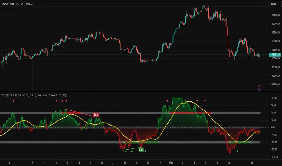
Seasonality Heatmap [QuantAlgo]🟢 Overview
The Seasonality Heatmap analyzes years of historical data to reveal which months and weekdays have consistently produced gains or losses, displaying results through color-coded tables with statistical metrics like consistency scores (1-10 rating) and positive occurrence rates. By calculating average returns for each calendar month and day-of-week combination, it identifies recognizable seasonal patterns (such as which months or weekdays tend to rally versus decline) and synthesizes this into actionable buy low/sell high timing possibilities for strategic entries and exits. This helps traders and investors spot high-probability seasonal windows where assets have historically shown strength or weakness, enabling them to align positions with recurring bull and bear market patterns.
🟢 How It Works
1. Monthly Heatmap
How % Return is Calculated:
The indicator fetches monthly closing prices (or Open/High/Low based on user selection) and calculates the percentage change from the previous month:
(Current Month Price - Previous Month Price) / Previous Month Price × 100
Each cell in the heatmap represents one month's return in a specific year, creating a multi-year historical view
Colors indicate performance intensity: greener/brighter shades for higher positive returns, redder/brighter shades for larger negative returns
What Averages Mean:
The "Avg %" row displays the arithmetic mean of all historical returns for each calendar month (e.g., averaging all Januaries together, all Februaries together, etc.)
This metric identifies historically recurring patterns by showing which months have tended to rise or fall on average
Positive averages indicate months that have typically trended upward; negative averages indicate historically weaker months
Example: If April shows +18.56% average, it means April has averaged a 18.56% gain across all years analyzed
What Months Up % Mean:
Shows the percentage of historical occurrences where that month had a positive return (closed higher than the previous month)
Calculated as:
(Number of Months with Positive Returns / Total Months) × 100
Values above 50% indicate the month has been positive more often than negative; below 50% indicates more frequent negative months
Example: If October shows "64%", then 64% of all historical Octobers had positive returns
What Consistency Score Means:
A 1-10 rating that measures how predictable and stable a month's returns have been
Calculated using the coefficient of variation (standard deviation / mean) - lower variation = higher consistency
High scores (8-10, green): The month has shown relatively stable behavior with similar outcomes year-to-year
Medium scores (5-7, gray): Moderate consistency with some variability
Low scores (1-4, red): High variability with unpredictable behavior across different years
Example: A consistency score of 8/10 indicates the month has exhibited recognizable patterns with relatively low deviation
What Best Means:
Shows the highest percentage return achieved for that specific month, along with the year it occurred
Reveals the maximum observed upside and identifies outlier years with exceptional performance
Useful for understanding the range of possible outcomes beyond the average
Example: "Best: 2016: +131.90%" means the strongest January in the dataset was in 2016 with an 131.90% gain
What Worst Means:
Shows the most negative percentage return for that specific month, along with the year it occurred
Reveals maximum observed downside and helps understand the range of historical outcomes
Important for risk assessment even in months with positive averages
Example: "Worst: 2022: -26.86%" means the weakest January in the dataset was in 2022 with a 26.86% loss
2. Day-of-Week Heatmap
How % Return is Calculated:
Calculates the percentage change from the previous day's close to the current day's price (based on user's price source selection)
Returns are aggregated by day of the week within each calendar month (e.g., all Mondays in January, all Tuesdays in January, etc.)
Each cell shows the average performance for that specific day-month combination across all historical data
Formula:
(Current Day Price - Previous Day Close) / Previous Day Close × 100
What Averages Mean:
The "Avg %" row at the bottom aggregates all months together to show the overall average return for each weekday
Identifies broad weekly patterns across the entire dataset
Calculated by summing all daily returns for that weekday across all months and dividing by total observations
Example: If Monday shows +0.04%, Mondays have averaged a 0.04% change across all months in the dataset
What Days Up % Mean:
Shows the percentage of historical occurrences where that weekday had a positive return
Calculated as:
(Number of Positive Days / Total Days Observed) × 100
Values above 50% indicate the day has been positive more often than negative; below 50% indicates more frequent negative days
Example: If Fridays show "54%", then 54% of all Fridays in the dataset had positive returns
What Consistency Score Means:
A 1-10 rating measuring how stable that weekday's performance has been across different months
Based on the coefficient of variation of daily returns for that weekday across all 12 months
High scores (8-10, green): The weekday has shown relatively consistent behavior month-to-month
Medium scores (5-7, gray): Moderate consistency with some month-to-month variation
Low scores (1-4, red): High variability across months, with behavior differing significantly by calendar month
Example: A consistency score of 7/10 for Wednesdays means they have performed with moderate consistency throughout the year
What Best Means:
Shows which calendar month had the strongest average performance for that specific weekday
Identifies favorable day-month combinations based on historical data
Format shows the month abbreviation and the average return achieved
Example: "Best: Oct: +0.20%" means Mondays averaged +0.20% during October months in the dataset
What Worst Means:
Shows which calendar month had the weakest average performance for that specific weekday
Identifies historically challenging day-month combinations
Useful for understanding which month-weekday pairings have shown weaker performance
Example: "Worst: Sep: -0.35%" means Tuesdays averaged -0.35% during September months in the dataset
3. Optimal Timing Table/Summary Table
→ Best Month to BUY: Identifies the month with the lowest average return (most negative or least positive historically), representing periods where prices have historically been relatively lower
Based on the observation that buying during historically weaker months may position for subsequent recovery
Shows the month name, its average return, and color-coded performance
Example: If May shows -0.86% as "Best Month to BUY", it means May has historically averaged -0.86% in the analyzed period
→ Best Month to SELL: Identifies the month with the highest average return (most positive historically), representing periods where prices have historically been relatively higher
Based on historical strength patterns in that month
Example: If July shows +1.42% as "Best Month to SELL", it means July has historically averaged +1.42% gains
→ 2nd Best Month to BUY: The second-lowest performing month based on average returns
Provides an alternative timing option based on historical patterns
Offers flexibility for staged entries or when the primary month doesn't align with strategy
Example: Identifies the next-most favorable historical buying period
→ 2nd Best Month to SELL: The second-highest performing month based on average returns
Provides an alternative exit timing based on historical data
Useful for staged profit-taking or multiple exit opportunities
Identifies the secondary historical strength period
Note: The same logic applies to "Best Day to BUY/SELL" and "2nd Best Day to BUY/SELL" rows, which identify weekdays based on average daily performance across all months. Days with lowest averages are marked as buying opportunities (historically weaker days), while days with highest averages are marked for selling (historically stronger days).
🟢 Examples
Example 1: NVIDIA NASDAQ:NVDA - Strong May Pattern with High Consistency
Analyzing NVIDIA from 2015 onwards, the Monthly Heatmap reveals May averaging +15.84% with 82% of months being positive and a consistency score of 8/10 (green). December shows -1.69% average with only 40% of months positive and a low 1/10 consistency score (red). The Optimal Timing table identifies December as "Best Month to BUY" and May as "Best Month to SELL." A trader recognizes this high-probability May strength pattern and considers entering positions in late December when prices have historically been weaker, then taking profits in May when the seasonal tailwind typically peaks. The high consistency score in May (8/10) provides additional confidence that this pattern has been relatively stable year-over-year.
Example 2: Crypto Market Cap CRYPTOCAP:TOTALES - October Rally Pattern
An investor examining total crypto market capitalization notices September averaging -2.42% with 45% of months positive and 5/10 consistency, while October shows a dramatic shift with +16.69% average, 90% of months positive, and an exceptional 9/10 consistency score (blue). The Day-of-Week heatmap reveals Mondays averaging +0.40% with 54% positive days and 9/10 consistency (blue), while Thursdays show only +0.08% with 1/10 consistency (yellow). The investor uses this multi-layered analysis to develop a strategy: enter crypto positions on Thursdays during late September (combining the historically weak month with the less consistent weekday), then hold through October's historically strong period, considering exits on Mondays when intraweek strength has been most consistent.
Example 3: Solana BINANCE:SOLUSDT - Extreme January Seasonality
A cryptocurrency trader analyzing Solana observes an extraordinary January pattern: +59.57% average return with 60% of months positive and 8/10 consistency (teal), while May shows -9.75% average with only 33% of months positive and 6/10 consistency. August also displays strength at +59.50% average with 7/10 consistency. The Optimal Timing table confirms May as "Best Month to BUY" and January as "Best Month to SELL." The Day-of-Week data shows Sundays averaging +0.77% with 8/10 consistency (teal). The trader develops a seasonal rotation strategy: accumulate SOL positions during May weakness, hold through the historically strong January period (which has shown this extreme pattern with reasonable consistency), and specifically target Sunday exits when the weekday data shows the most recognizable strength pattern.

Stochastic Enhanced [DCAUT]█ Stochastic Enhanced
📊 ORIGINALITY & INNOVATION
The Stochastic Enhanced indicator builds upon George Lane's classic momentum oscillator (developed in the late 1950s) by providing comprehensive smoothing algorithm flexibility. While traditional implementations limit users to Simple Moving Average (SMA) smoothing, this enhanced version offers 21 advanced smoothing algorithms, allowing traders to optimize the indicator's characteristics for different market conditions and trading styles.
Key Improvements:
Extended from single SMA smoothing to 21 professional-grade algorithms including adaptive filters (KAMA, FRAMA), zero-lag methods (ZLEMA, T3), and advanced digital filters (Kalman, Laguerre)
Maintains backward compatibility with traditional Stochastic calculations through SMA default setting
Unified smoothing algorithm applies to both %K and %D lines for consistent signal processing characteristics
Enhanced visual feedback with clear color distinction and background fill highlighting for intuitive signal recognition
Comprehensive alert system covering crossovers and zone entries for systematic trade management
Differentiation from Traditional Stochastic:
Traditional Stochastic indicators use fixed SMA smoothing, which introduces consistent lag regardless of market volatility. This enhanced version addresses the limitation by offering adaptive algorithms that adjust to market conditions (KAMA, FRAMA), reduce lag without sacrificing smoothness (ZLEMA, T3, HMA), or provide superior noise filtering (Kalman Filter, Laguerre filters). The flexibility helps traders balance responsiveness and stability according to their specific needs.
📐 MATHEMATICAL FOUNDATION
Core Stochastic Calculation:
The Stochastic Oscillator measures the position of the current close relative to the high-low range over a specified period:
Step 1: Raw %K Calculation
%K_raw = 100 × (Close - Lowest Low) / (Highest High - Lowest Low)
Where:
Close = Current closing price
Lowest Low = Lowest low over the %K Length period
Highest High = Highest high over the %K Length period
Result ranges from 0 (close at period low) to 100 (close at period high)
Step 2: Smoothed %K Calculation
%K = MA(%K_raw, K Smoothing Period, MA Type)
Where:
MA = Selected moving average algorithm (SMA, EMA, etc.)
K Smoothing = 1 for Fast Stochastic, 3+ for Slow Stochastic
Traditional Fast Stochastic uses %K_raw directly without smoothing
Step 3: Signal Line %D Calculation
%D = MA(%K, D Smoothing Period, MA Type)
Where:
%D acts as a signal line and moving average of %K
D Smoothing typically set to 3 periods in traditional implementations
Both %K and %D use the same MA algorithm for consistent behavior
Available Smoothing Algorithms (21 Options):
Standard Moving Averages:
SMA (Simple): Equal-weighted average, traditional default, consistent lag characteristics
EMA (Exponential): Recent price emphasis, faster response to changes, exponential decay weighting
RMA (Rolling/Wilder's): Smoothed average used in RSI, less reactive than EMA
WMA (Weighted): Linear weighting favoring recent data, moderate responsiveness
VWMA (Volume-Weighted): Incorporates volume data, reflects market participation intensity
Advanced Moving Averages:
HMA (Hull): Reduced lag with smoothness, uses weighted moving averages and square root period
ALMA (Arnaud Legoux): Gaussian distribution weighting, minimal lag with good noise reduction
LSMA (Least Squares): Linear regression based, fits trend line to data points
DEMA (Double Exponential): Reduced lag compared to EMA, uses double smoothing technique
TEMA (Triple Exponential): Further lag reduction, triple smoothing with lag compensation
ZLEMA (Zero-Lag Exponential): Lag elimination attempt using error correction, very responsive
TMA (Triangular): Double-smoothed SMA, very smooth but slower response
Adaptive & Intelligent Filters:
T3 (Tilson T3): Six-pass exponential smoothing with volume factor adjustment, excellent smoothness
FRAMA (Fractal Adaptive): Adapts to market fractal dimension, faster in trends, slower in ranges
KAMA (Kaufman Adaptive): Efficiency ratio based adaptation, responds to volatility changes
McGinley Dynamic: Self-adjusting mechanism following price more accurately, reduced whipsaws
Kalman Filter: Optimal estimation algorithm from aerospace engineering, dynamic noise filtering
Advanced Digital Filters:
Ultimate Smoother: Advanced digital filter design, superior noise rejection with minimal lag
Laguerre Filter: Time-domain filter with N-order implementation, adjustable lag characteristics
Laguerre Binomial Filter: 6-pole Laguerre filter, extremely smooth output for long-term analysis
Super Smoother: Butterworth filter implementation, removes high-frequency noise effectively
📊 COMPREHENSIVE SIGNAL ANALYSIS
Absolute Level Interpretation (%K Line):
%K Above 80: Overbought condition, price near period high, potential reversal or pullback zone, caution for new long entries
%K in 70-80 Range: Strong upward momentum, bullish trend confirmation, uptrend likely continuing
%K in 50-70 Range: Moderate bullish momentum, neutral to positive outlook, consolidation or mild uptrend
%K in 30-50 Range: Moderate bearish momentum, neutral to negative outlook, consolidation or mild downtrend
%K in 20-30 Range: Strong downward momentum, bearish trend confirmation, downtrend likely continuing
%K Below 20: Oversold condition, price near period low, potential bounce or reversal zone, caution for new short entries
Crossover Signal Analysis:
%K Crosses Above %D (Bullish Cross): Momentum shifting bullish, faster line overtakes slower signal, consider long entry especially in oversold zone, strongest when occurring below 20 level
%K Crosses Below %D (Bearish Cross): Momentum shifting bearish, faster line falls below slower signal, consider short entry especially in overbought zone, strongest when occurring above 80 level
Crossover in Midrange (40-60): Less reliable signals, often in choppy sideways markets, require additional confirmation from trend or volume analysis
Multiple Failed Crosses: Indicates ranging market or choppy conditions, reduce position sizes or avoid trading until clear directional move
Advanced Divergence Patterns (%K Line vs Price):
Bullish Divergence: Price makes lower low while %K makes higher low, indicates weakening bearish momentum, potential trend reversal upward, more reliable when %K in oversold zone
Bearish Divergence: Price makes higher high while %K makes lower high, indicates weakening bullish momentum, potential trend reversal downward, more reliable when %K in overbought zone
Hidden Bullish Divergence: Price makes higher low while %K makes lower low, indicates trend continuation in uptrend, bullish trend strength confirmation
Hidden Bearish Divergence: Price makes lower high while %K makes higher high, indicates trend continuation in downtrend, bearish trend strength confirmation
Momentum Strength Analysis (%K Line Slope):
Steep %K Slope: Rapid momentum change, strong directional conviction, potential for extended moves but also increased reversal risk
Gradual %K Slope: Steady momentum development, sustainable trends more likely, lower probability of sharp reversals
Flat or Horizontal %K: Momentum stalling, potential reversal or consolidation ahead, wait for directional break before committing
%K Oscillation Within Range: Indicates ranging market, sideways price action, better suited for range-trading strategies than trend following
🎯 STRATEGIC APPLICATIONS
Mean Reversion Strategy (Range-Bound Markets):
Identify ranging market conditions using price action or Bollinger Bands
Wait for Stochastic to reach extreme zones (above 80 for overbought, below 20 for oversold)
Enter counter-trend position when %K crosses %D in extreme zone (sell on bearish cross above 80, buy on bullish cross below 20)
Set profit targets near opposite extreme or midline (50 level)
Use tight stop-loss above recent swing high/low to protect against breakout scenarios
Exit when Stochastic reaches opposite extreme or %K crosses %D in opposite direction
Trend Following with Momentum Confirmation:
Identify primary trend direction using higher timeframe analysis or moving averages
Wait for Stochastic pullback to oversold zone (<20) in uptrend or overbought zone (>80) in downtrend
Enter in trend direction when %K crosses %D confirming momentum shift (bullish cross in uptrend, bearish cross in downtrend)
Use wider stops to accommodate normal trend volatility
Add to position on subsequent pullbacks showing similar Stochastic pattern
Exit when Stochastic shows opposite extreme with failed cross or bearish/bullish divergence
Divergence-Based Reversal Strategy:
Scan for divergence between price and Stochastic at swing highs/lows
Confirm divergence with at least two price pivots showing divergent Stochastic readings
Wait for %K to cross %D in direction of anticipated reversal as entry trigger
Enter position in divergence direction with stop beyond recent swing extreme
Target profit at key support/resistance levels or Fibonacci retracements
Scale out as Stochastic reaches opposite extreme zone
Multi-Timeframe Momentum Alignment:
Analyze Stochastic on higher timeframe (4H or Daily) for primary trend bias
Switch to lower timeframe (1H or 15M) for precise entry timing
Only take trades where lower timeframe Stochastic signal aligns with higher timeframe momentum direction
Higher timeframe Stochastic in bullish zone (>50) = only take long entries on lower timeframe
Higher timeframe Stochastic in bearish zone (<50) = only take short entries on lower timeframe
Exit when lower timeframe shows counter-signal or higher timeframe momentum reverses
Zone Transition Strategy:
Monitor Stochastic for transitions between zones (oversold to neutral, neutral to overbought, etc.)
Enter long when Stochastic crosses above 20 (exiting oversold), signaling momentum shift from bearish to neutral/bullish
Enter short when Stochastic crosses below 80 (exiting overbought), signaling momentum shift from bullish to neutral/bearish
Use zone midpoint (50) as dynamic support/resistance for position management
Trail stops as Stochastic advances through favorable zones
Exit when Stochastic fails to maintain momentum and reverses back into prior zone
📋 DETAILED PARAMETER CONFIGURATION
%K Length (Default: 14):
Lower Values (5-9): Highly sensitive to price changes, generates more frequent signals, increased false signals in choppy markets, suitable for very short-term trading and scalping
Standard Values (10-14): Balanced sensitivity and reliability, traditional default (14) widely used,适合 swing trading and intraday strategies
Higher Values (15-21): Reduced sensitivity, smoother oscillations, fewer but potentially more reliable signals, better for position trading and lower timeframe noise reduction
Very High Values (21+): Slow response, long-term momentum measurement, fewer trading signals, suitable for weekly or monthly analysis
%K Smoothing (Default: 3):
Value 1: Fast Stochastic, uses raw %K calculation without additional smoothing, most responsive to price changes, generates earliest signals with higher noise
Value 3: Slow Stochastic (default), traditional smoothing level, reduces false signals while maintaining good responsiveness, widely accepted standard
Values 5-7: Very slow response, extremely smooth oscillations, significantly reduced whipsaws but delayed entry/exit timing
Recommendation: Default value 3 suits most trading scenarios, active short-term traders may use 1, conservative long-term positions use 5+
%D Smoothing (Default: 3):
Lower Values (1-2): Signal line closely follows %K, frequent crossover signals, useful for active trading but requires strict filtering
Standard Value (3): Traditional setting providing balanced signal line behavior, optimal for most trading applications
Higher Values (4-7): Smoother signal line, fewer crossover signals, reduced whipsaws but slower confirmation, better for trend trading
Very High Values (8+): Signal line becomes slow-moving reference, crossovers rare and highly significant, suitable for long-term position changes only
Smoothing Type Algorithm Selection:
For Trending Markets:
ZLEMA, DEMA, TEMA: Reduced lag for faster trend entry, quick response to momentum shifts, suitable for strong directional moves
HMA, ALMA: Good balance of smoothness and responsiveness, effective for clean trend following without excessive noise
EMA: Classic choice for trending markets, faster than SMA while maintaining reasonable stability
For Ranging/Choppy Markets:
Kalman Filter, Super Smoother: Superior noise filtering, reduces false signals in sideways action, helps identify genuine reversal points
Laguerre Filters: Smooth oscillations with adjustable lag, excellent for mean reversion strategies in ranges
T3, TMA: Very smooth output, filters out market noise effectively, clearer extreme zone identification
For Adaptive Market Conditions:
KAMA: Automatically adjusts to market efficiency, fast in trends and slow in congestion, reduces whipsaws during transitions
FRAMA: Adapts to fractal market structure, responsive during directional moves, conservative during uncertainty
McGinley Dynamic: Self-adjusting smoothing, follows price naturally, minimizes lag in trending markets while filtering noise in ranges
For Conservative Long-Term Analysis:
SMA: Traditional choice, predictable behavior, widely understood characteristics
RMA (Wilder's): Smooth oscillations, reduced sensitivity to outliers, consistent behavior across market conditions
Laguerre Binomial Filter: Extremely smooth output, ideal for weekly/monthly timeframe analysis, eliminates short-term noise completely
Source Selection:
Close (Default): Standard choice using closing prices, most common and widely tested
HLC3 or OHLC4: Incorporates more price information, reduces impact of sudden spikes or gaps, smoother oscillator behavior
HL2: Midpoint of high-low range, emphasizes intrabar volatility, useful for markets with wide intraday ranges
Custom Source: Can use other indicators as input (e.g., Heikin Ashi close, smoothed price), creates derivative momentum indicators
📈 PERFORMANCE ANALYSIS & COMPETITIVE ADVANTAGES
Responsiveness Characteristics:
Traditional SMA-Based Stochastic:
Fixed lag regardless of market conditions, consistent delay of approximately (K Smoothing + D Smoothing) / 2 periods
Equal treatment of trending and ranging markets, no adaptation to volatility changes
Predictable behavior but suboptimal in varying market regimes
Enhanced Version with Adaptive Algorithms:
KAMA and FRAMA reduce lag by up to 40-60% in strong trends compared to SMA while maintaining similar smoothness in ranges
ZLEMA and T3 provide near-zero lag characteristics for early entry signals with acceptable noise levels
Kalman Filter and Super Smoother offer superior noise rejection, reducing false signals in choppy conditions by estimations of 30-50% compared to SMA
Performance improvements vary by algorithm selection and market conditions
Signal Quality Improvements:
Adaptive algorithms help reduce whipsaw trades in ranging markets by adjusting sensitivity dynamically
Advanced filters (Kalman, Laguerre, Super Smoother) provide clearer extreme zone readings for mean reversion strategies
Zero-lag methods (ZLEMA, DEMA, TEMA) generate earlier crossover signals in trending markets for improved entry timing
Smoother algorithms (T3, Laguerre Binomial) reduce false extreme zone touches for more reliable overbought/oversold signals
Comparison with Standard Implementations:
Versus Basic Stochastic: Enhanced version offers 21 smoothing options versus single SMA, allowing optimization for specific market characteristics and trading styles
Versus RSI: Stochastic provides range-bound measurement (0-100) with clear extreme zones, RSI measures momentum speed, Stochastic offers clearer visual overbought/oversold identification
Versus MACD: Stochastic bounded oscillator suitable for mean reversion, MACD unbounded indicator better for trend strength, Stochastic excels in range-bound and oscillating markets
Versus CCI: Stochastic has fixed bounds (0-100) for consistent interpretation, CCI unbounded with variable extremes, Stochastic provides more standardized extreme readings across different instruments
Flexibility Advantages:
Single indicator adaptable to multiple strategies through algorithm selection rather than requiring different indicator variants
Ability to optimize smoothing characteristics for specific instruments (e.g., smoother for crypto volatility, faster for forex trends)
Multi-timeframe analysis with consistent algorithm across timeframes for coherent momentum picture
Backtesting capability with algorithm as optimization parameter for strategy development
Limitations and Considerations:
Increased complexity from multiple algorithm choices may lead to over-optimization if parameters are curve-fitted to historical data
Adaptive algorithms (KAMA, FRAMA) have adjustment periods during market regime changes where signals may be less reliable
Zero-lag algorithms sacrifice some smoothness for responsiveness, potentially increasing noise sensitivity in very choppy conditions
Performance characteristics vary significantly across algorithms, requiring understanding and testing before live implementation
Like all oscillators, Stochastic can remain in extreme zones for extended periods during strong trends, generating premature reversal signals
USAGE NOTES
This indicator is designed for technical analysis and educational purposes to provide traders with enhanced flexibility in momentum analysis. The Stochastic Oscillator has limitations and should not be used as the sole basis for trading decisions.
Important Considerations:
Algorithm performance varies with market conditions - no single smoothing method is optimal for all scenarios
Extreme zone signals (overbought/oversold) indicate potential reversal areas but not guaranteed turning points, especially in strong trends
Crossover signals may generate false entries during sideways choppy markets regardless of smoothing algorithm
Divergence patterns require confirmation from price action or additional indicators before trading
Past indicator characteristics and backtested results do not guarantee future performance
Always combine Stochastic analysis with proper risk management, position sizing, and multi-indicator confirmation
Test selected algorithm on historical data of specific instrument and timeframe before live trading
Market regime changes may require algorithm adjustment for optimal performance
The enhanced smoothing options are intended to provide tools for optimizing the indicator's behavior to match individual trading styles and market characteristics, not to create a perfect predictive tool. Responsible usage includes understanding the mathematical properties of selected algorithms and their appropriate application contexts.

Natural Gas Intraday Strategy [15m] with Partial Profit & TrailBuy when:
1. Close > EMA 100 and EMA 20 > EMA 100
2. MACD (8,21,5) > Signal and histogram rising
3. RSI > 60
4. ATR > threshold (avoid flat market)
Sell when:
1. Close < EMA 100 and EMA 20 < EMA 100
2. MACD (8,21,5) < Signal and histogram falling
3. RSI < 40
4. ATR > threshold
Exit:
• SL = recent swing ± 0.5 ATR
• TP1 = 1 ATR, trail rest with EMA 20

Multi-Timeframe Trend Table - EMA Based Trend Analysis📊 Stay Aligned with Higher Timeframe Trends While Scalping
This powerful indicator displays real-time trend direction for 1-hour and 4-hour timeframes in a clean, easy-to-read table format. Perfect for traders who want to align their short-term trades with higher timeframe momentum.
🎯 Key Features
Multi-Timeframe Analysis: Monitor 1H and 4H trends while trading on any timeframe (3min, 5min, 15min, etc.)
EMA-Based Logic: Uses proven EMA 50 and EMA 100 crossover methodology
Visual Clarity: Color-coded table with green (uptrend) and red (downtrend) indicators
Customizable Display: Toggle EMA values and adjust table position
Real-Time Updates: Automatically refreshes with each bar close
Lightweight: Minimal resource usage with efficient data requests
📈 How It Works
The indicator determines trend direction using a simple but effective rule:
UPTREND: Price is above both EMA 50 AND EMA 100
DOWNTREND: Price is below either EMA 50 OR EMA 100
🔧 Settings
Show EMA Values: Display actual EMA 50/100 values in the table
Table Position: Choose from 4 corner positions (Top Right, Top Left, Bottom Right, Bottom Left)
Plot Current EMAs: Optional display of EMA lines on your current chart
💡 Trading Applications
✅ Trend Confirmation: Ensure your trades align with higher timeframe direction
✅ Risk Management: Avoid counter-trend trades in strong directional markets
✅ Entry Timing: Use lower timeframe for entries while respecting higher timeframe bias
✅ Scalping Enhancement: Perfect for 1-5 minute scalping with higher timeframe context
🎨 Visual Design
Clean, professional table design
Intuitive color coding (Green = Up, Red = Down)
Compact size that doesn't obstruct your chart
Clear typography for quick reading
📋 Perfect For
Day traders and scalpers
Swing traders seeking trend confirmation
Multi-timeframe analysis enthusiasts
Traders who want simple, effective trend identification
🚀 Easy Setup
Add to any chart (works on all timeframes)
Customize table position and settings
Start trading with higher timeframe awareness
Watch the table update automatically
No complex configurations needed - just add and trade!
This indicator is designed for educational and informational purposes. Always combine with proper risk management and your own analysis.
