Bias + VWAP Pullback — v4 (PA + BOS/CHOCH)Simple idea: I identify the trend (bias) from the larger timeframe, and only trade pullbacks to the VWAP/EMA during liquidity (London/New York). When the trend is clear, gold moves strongly, and its pullbacks to the balance lines provide clear opportunities.
Timeframe and Sessions (Cairo Time)
Analysis: H1 to determine the trend.
Implementation: 5m (or 1m if professional).
Trading window:
London Opening: 10:00–12:30
New York Opening: 16:30–19:00
(avoid the rest of the day unless there is exceptional traffic).
Direction determination (BIAS)
On H1:
If the price is above the 200 EMA and the daily VWAP is bullish and the price is above it → uptrend (long-only).
If the price is below the 200 EMA and the daily VWAP is bearish and the price is below it → bearish trend (short-only).
Determine your levels: yesterday's high/low (PDH/PDL) + approximate Asia range (03:00–09:30).
Entry Rules (Setup A: Trend Continuation)
Asia range breakout towards Bias during liquidity window.
Wait for a withdrawal to:
Daily VWAP, or
EMA50 on 5m frame (best if both cross).
Confirmation: Confirmation low/high on 5m (HL buy/LH sell) + clear impulse candle (Body is greater than average of last 10 candles).
Entry:
Buy: When the price returns above VWAP/EMA50 with a confirmation candle close.
Sell: The exact opposite.
Stop Loss (SL): Below/above the last confirmation low/high or ATR(14, 5m) x 1.5 (largest).
Objectives:
TP1 = 1R (Close 50% and move the rest Break-even).
TP2 = 2.5R to 3R or at an important HTF level (PDH/PDL/Bid/Demand Zone).
Entry Rules (Setup B: Reversion to VWAP – “Mean Reversion”)
Use with extreme caution, once daily maximum:
Price deviation from VWAP by more than ~1.5 x ATR(14, 5m) with rejection candles appearing near PDH/PDL.
Reverse entry towards the return of VWAP.
SL small behind rejection top/bottom.
Main target: VWAP. (Don't get greedy — this scenario is for extended periods only.)
News Filtering and Risk Management
Avoid trading 15–30 minutes before/after strong US news (CPI, NFP, FOMC).
Maximum daily loss: 1.5–2% of account balance.
Risk per trade: 0.25–0.5% (if you are learning) or 0.5–1% (if you are experienced).
Do not exceed two consecutive losing trades per day.
Don't chase the market after the opportunity has passed — wait for the next pullback.
Smart Deal Management
After TP1: Move stop to entry point + trail the rest with EMA20 on 5m or ATR Trailing = ATR(14)×1.0.
If the price touches a strong daily level (PDH/PDL) and fails to break, consider taking additional profit.
If VWAP starts to flatten and breaks against the trend on H1, stop trading for the day.
Quick Checklist (Before Entry)
H1 trend is clear and consistent with 200EMA + VWAP.
Penetrating the Asia range towards Bias.
Clean pull to VWAP/EMA50 on 5m.
Confirmation candle and real push.
SL is logical (behind swing/ATR×1.5) and R :R ≥ 1:2.
No red news coming soon.
Example of "ready-made" settings
EMA: 20, 50, 200 on 5m, 200 only on H1.
VWAP: Daily (reset daily).
ATR: 14 on 5m.
Levels: PDH/PDL + Asia Band (03:00–09:30 Cairo).
Gold Notes
Gold is fast and sharp at the open; don't get in early — wait for the draw.
Fakeouts are common before news: it is best to call with the trend after the price returns above/below VWAP.
Don't expect 80% consistent wins every day — the advantage comes from discipline, filtering out bad days, and only withdrawing when you're on the right track.
تعتبر شركة الماسة الألمانية أحد المؤسسات العاملة بالمملكة العربية السعودية ولها تاريخ طويل من الخدمات الكثيرة والمتنوعة التى مازالت تقدمها للكثير من العملاء داخل جميع مدن وأحياء المملكة حيث نقدم أفضل ما لدينا من خلال مجموعة الشركات التالية والتي من خلالها ستتلقي كل ما تحتاج إلية في كل المجال المختلفة فنحن نعمل منذ عام 2015 ولنا سابقات اعمال فى مختلف المجالات الحيوية التى نخدم من خلالها عملائنا ونوفر لهم أرخص الأسعار وبأعلى جودة من الممكن توفرها فى المجالات التالية :-
خدمات تنظيف المنازل والفلل والشقق
خدمات عزل الخزانات تنظيف غسيل صيانة اصلاح
خدمات جلي البلاط والرخام والسيراميك
خدمات نقل العفش عمالة فلبينية مدربة
خدمات مكافحة الحشرات بجدة
كل هذة الخدمات وأكثر نوفرها لكل المتعاقدين بأفضل الطرق مع توفير خطط وبرامج متنوعة لأتمام العمل المسنود إلينا بأفضل وأحدث الطرق الحديثة والعصرية سواء فى شركات النظافة بجدة ومكة المكرمة أو شركات نقل العفش بجدة عمالة فلبينية وباقى الخدمات مثل جلي وتلميع الرخام بمكة وجدة ولا ننسي شركة مكافحة حشرات بجدة التى ساعدت آلاف المواطنين على تنظيف منازلهم من الحشرات بأفضل مبيدات حشرية.
In den Scripts nach "央行:下调个人住房公积金贷款利率0.25个百分点" suchen

TRI - Multi-Timeframe BIASTRI - MULTI-TIMEFRAME BIAS INDICATOR
DESCRIPTION:
Advanced multi-timeframe bias indicator that analyzes market sentiment across
5 different timeframes (15m, 1h, 4h, 1d, 1w) using adaptive technical analysis.
Provides clear directional bias signals to help determine market momentum.
KEY FEATURES:
ADAPTIVE PARAMETERS: Uses different EMA lengths and weights for each timeframe
EMA TREND ANALYSIS: Fast/slow EMA crossovers with slope analysis for momentum
RSI MOMENTUM: Adaptive overbought/oversold levels based on timeframe
ADX STRENGTH: Directional movement confirmation with DI+/DI- analysis
COMPOSITE SCORING: Weighted combination of trend, momentum, and strength
TIMEFRAME ANALYSIS:
15m: EMA9/21 + High momentum weight (45%) - Ultra-responsive for scalping
1h: EMA21/50 + Medium momentum weight (35%) - Balanced for day trading
4h: EMA50/200 + Lower momentum weight (25%) - Swing trading focus
1d: EMA50/200 + Trend focused (55%) - Position trading signals
1w: EMA50/200 + Maximum trend weight (60%) - Long-term bias
BIAS SIGNALS:
STRONG BULLISH/BEARISH: Score ≥ 0.5 - Very strong directional momentum
BULLISH/BEARISH: Score ≥ 0.25 - Clear directional signals
WEAK BULLISH/BEARISH: Score ≥ 0.1 - Mild directional bias
NEUTRAL: Score < 0.1 - No clear directional preference
ALERTS:
Major Bullish/Bearish: When 4H and 1D timeframes align
High confidence signals for strategic decision making
USAGE:
Higher timeframes (1d, 1w) show primary market direction
Lower timeframes (15m, 1h) provide entry timing
Look for alignment across multiple timeframes for stronger signals
Use confidence levels to assess signal reliability
TECHNICAL COMPONENTS:
Exponential Moving Averages (EMA) for responsive trend detection
Relative Strength Index (RSI) for momentum analysis
Average Directional Index (ADX) with DI+/DI- for trend strength
Volume ratio confirmation for signal validation
Adaptive thresholds optimized for each timeframe's characteristics

Gann Fan Strategy [KedarArc Quant]Description
A single-concept, rule-based strategy that trades around a programmatic Gann Fan.
It anchors to a swing (or a manual point), builds 1×1 and related fan lines numerically, and triggers entries when price interacts with the 1×1 (breakout or bounce). Management is done entirely with the fan structure (next/previous line) plus optional ATR trailing.
What TV indicators are used
* Pivots: `ta.pivothigh/ta.pivotlow` to confirm swing highs/lows for anchor selection.
* ATR: `ta.atr` only to scale the 1×1 slope (optional) and for an optional trailing stop.
* EMA: `ta.ema` as a trend filter (e.g., only long above the EMA, short below).
No RSI/MACD/Stoch/Heikin/etc. The logic is one coherent framework: Gann price–time geometry, with ATR as a scale and EMA as a risk filter.
How it works
1. Anchor
* Auto: chooses the most recent *confirmed* pivot (you control Left/Right).
* Manual: set a price and bar index and the fan will hold that point (no re-anchoring).
* Optional Re-anchor when a newer pivot confirms.
2. 1×1 Slope (numeric, not cosmetic)
* ATR mode: `1×1 = ATR(Length) × Multiplier` (adapts to volatility).
* Fixed mode: `ticks per bar` (constant slope).
Because slope is numeric, it doesn’t change with chart zoom, unlike the drawing tool.
3. Fan Lines
Builds classic ratios around the 1×1: 1/8, 1/4, 1/3, 1/2, 1/1, 2/1, 3/1, 4/1, 8/1.
4. Signals
* Breakout: cross of price over/under the 1×1 in the EMA-aligned direction.
* Bounce (optional): touch + reversal across the 1×1 to reduce whipsaw.
5. Exits & Risk
* Take-profit at the next fan line; Stop at the previous fan line.
* If a level is missing (right after re-anchor), a fallback Risk-Reward (RR) is used.
* Optional ATR trailing stop.
Why this is unique
* True numeric fan: The 1×1 slope is calculated from ATR or fixed ticks—not from screen geometry—so it is scale-invariant and reproducible across users/timeframes.
* Deterministic anchor logic: Uses confirmed pivots (with your L/R settings). No look-ahead; anchors update only when the right bars complete.
* Fan-native trade management: Both entries and exits come from the fan structure itself (with a minimal ATR/EMA assist), keeping the method pure.
* Two entry archetypes: Breakout for momentum days; Bounce for range days—switchable without changing the core model.
* Manual mode: Lock a session’s bias by anchoring to a chosen swing (e.g., day’s first major low/high) and keep the fan constant all day.
Inputs (quick guide)
* Auto Anchor (Left/Right): pivot sensitivity. Higher values = fewer, stronger anchors.
* Re-anchor: refresh to newer pivots as they confirm.
* Manual Anchor Price / Bar Index: fixes the fan (turn Auto off).
* Scale 1×1 by ATR: on = adaptive; off = use ticks per bar.
* ATR Length / ATR Multiplier: controls adaptive slope; start around 14 / 0.25–0.35.
* Ticks per bar: exact fixed slope (match a hand-drawn fan by computing slope ÷ mintick).
* EMA Trend Filter: e.g., 50–100; trades only in EMA direction.
* Use Bounce: require touch + reverse across 1×1 (helps in chop).
* TP/SL at fan lines; Fallback RR for missing levels; ATR Trailing Stop optional.
* Transparency/Plot EMA: visual preferences.
Tips
* Range days: larger pivots (L/R 8–12), Bounce ON, ATR Multiplier \~0.30–0.40, EMA 100.
* Trend days: L/R 5–6, Breakout, Multiplier \~0.20–0.30, EMA 50, ATR trail 1.0–1.5.
* Match the TV Gann Fan drawing: turn ATR scale OFF, set ticks per bar = `(Δprice between anchor and 1×1 target) / (bars) / mintick`.
Repainting & testing notes
* Pivots require Right bars to confirm; anchors are set after confirmation (no look-ahead).
* Signals use the current bar close with TradingView strategy mechanics; real-time vs. bar-close can differ slightly, as with any strategy.
* Re-anchoring legitimately moves the structure when new pivots confirm—by design.
⚠️ Disclaimer
This script is provided for educational purposes only.
Past performance does not guarantee future results.
Trading involves risk, and users should exercise caution and use proper risk management when applying this strategy.

Deadband Hysteresis Filter [BackQuant]Deadband Hysteresis Filter
What this is
This tool builds a “debounced” price baseline that ignores small fluctuations and only reacts when price meaningfully departs from its recent path. It uses a deadband to define how much deviation matters and a hysteresis scheme to avoid rapid flip-flops around the decision boundary. The baseline’s slope provides a simple trend cue, used to color candles and to trigger up and down alerts.
Why deadband and hysteresis help
They filter micro noise so the baseline does not react to every tiny tick.
They stabilize state changes. Hysteresis means the rule to start moving is stricter than the rule to keep holding, which reduces whipsaw.
They produce a stepped, readable path that advances during sustained moves and stays flat during chop.
How it works (conceptual)
At each bar the script maintains a running baseline dbhf and compares it to the input price p .
Compute a base threshold baseTau using the selected mode (ATR, Percent, Ticks, or Points).
Build an enter band tauEnter = baseTau × Enter Mult and an exit band tauExit = baseTau × Exit Mult where typically Exit Mult < Enter Mult .
Let diff = p − dbhf .
If diff > +tauEnter , raise the baseline by response × (diff − tauEnter) .
If diff < −tauEnter , lower the baseline by response × (diff + tauEnter) .
Otherwise, hold the prior value.
Trend state is derived from slope: dbhf > dbhf → up trend, dbhf < dbhf → down trend.
Inputs and what they control
Threshold mode
ATR — baseTau = ATR(atrLen) × atrMult . Adapts to volatility. Useful when regimes change.
Percent — baseTau = |price| × pctThresh% . Scale-free across symbols of different prices.
Ticks — baseTau = syminfo.mintick × tickThresh . Good for futures where tick size matters.
Points — baseTau = ptsThresh . Fixed distance in price units.
Band multipliers and response
Enter Mult — outer band. Price must travel at least this far from the baseline before an update occurs. Larger values reject more noise but increase lag.
Exit Mult — inner band for hysteresis. Keep this smaller than Enter Mult to create a hold zone that resists small re-entries.
Response — step size when outside the enter band. Higher response tracks faster; lower response is smoother.
UI settings
Show Filtered Price — plots the baseline on price.
Paint candles — colors bars by the filtered slope using your long/short colors.
How it can be used
Trend qualifier — take entries only in the direction of the baseline slope and skip trades against it.
Debounced crossovers — use the baseline as a stabilized surrogate for price in moving-average or channel crossover rules.
Trailing logic — trail stops a small distance beyond the baseline so small pullbacks do not eject the trade.
Session aware filtering — widen Enter Mult or switch to ATR mode for volatile sessions; tighten in quiet sessions.
Parameter interactions and tuning
Enter Mult vs Response — both govern sensitivity. If you see too many flips, increase Enter Mult or reduce Response. If turns feel late, do the opposite.
Exit Mult — widening the gap between Enter and Exit expands the hold zone and reduces oscillation around the threshold.
Mode choice — ATR adapts automatically; Percent keeps behavior consistent across instruments; Ticks or Points are useful when you think in fixed increments.
Timeframe coupling — on higher timeframes you can often lower Enter Mult or raise Response because raw noise is already reduced.
Concrete starter recipes
General purpose — ATR mode, atrLen=14 , atrMult=1.0–1.5 , Enter=1.0 , Exit=0.5 , Response=0.20 . Balanced noise rejection and lag.
Choppy range filter — ATR mode, increase atrMult to 2.0, keep Response≈0.15 . Stronger suppression of micro-moves.
Fast intraday — Percent mode, pctThresh=0.1–0.3 , Enter=1.0 , Exit=0.4–0.6 , Response=0.30–0.40 . Quicker turns for scalping.
Futures ticks — Ticks mode, set tickThresh to a few spreads beyond typical noise; start with Enter=1.0 , Exit=0.5 , Response=0.25 .
Strengths
Clear, explainable logic with an explicit noise budget.
Multiple threshold modes so the same tool fits equities, futures, and crypto.
Built-in hysteresis that reduces flip-flop near the boundary.
Slope-based coloring and alerts that make state changes obvious in real time.
Limitations and notes
All filters add lag. Larger thresholds and smaller response trade faster reaction for fewer false turns.
Fixed Points or Ticks can under- or over-filter when volatility regime shifts. ATR adapts, but will also expand bands during spikes.
On extremely choppy symbols, even a well tuned band will step frequently. Widen Enter Mult or reduce Response if needed.
This is a chart study. It does not include commissions, slippage, funding, or gap risks.
Alerts
DBHF Up Slope — baseline turns from down to up on the latest bar.
DBHF Down Slope — baseline turns from up to down on the latest bar.
Implementation details worth knowing
Initialization sets the baseline to the first observed price to avoid a cold-start jump.
Slope is evaluated bar-to-bar. The up and down alerts check for a change of slope rather than raw price crossings.
Candle colors and the baseline plot share the same long/short palette with transparency applied to the line.
Practical workflow
Pick a mode that matches how you think about distance. ATR for volatility aware, Percent for scale-free, Ticks or Points for fixed increments.
Tune Enter Mult until the number of flips feels appropriate for your timeframe.
Set Exit Mult clearly below Enter Mult to create a real hold zone.
Adjust Response last to control “how fast” the baseline chases price once it decides to move.
Final thoughts
Deadband plus hysteresis gives you a principled way to “only care when it matters.” With a sensible threshold and response, the filter yields a stable, low-chop trend cue you can use directly for bias or plug into your own entries, exits, and risk rules.

Market Outlook Score (MOS)Overview
The "Market Outlook Score (MOS)" is a custom technical indicator designed for TradingView, written in Pine Script version 6. It provides a quantitative assessment of market conditions by aggregating multiple factors, including trend strength across different timeframes, directional movement (via ADX), momentum (via RSI changes), volume dynamics, and volatility stability (via ATR). The MOS is calculated as a weighted score that ranges typically between -1 and +1 (though it can exceed these bounds in extreme conditions), where positive values suggest bullish (long) opportunities, negative values indicate bearish (short) setups, and values near zero imply neutral or indecisive markets.
This indicator is particularly useful for traders seeking a holistic "outlook" score to gauge potential entry points or market bias. It overlays on a separate pane (non-overlay mode) and visualizes the score through horizontal threshold lines and dynamic labels showing the numeric MOS value along with a simple trading decision ("Long", "Short", or "Neutral"). The script avoids using the plot function for compatibility reasons (e.g., potential TradingView bugs) and instead relies on hline for static lines and label.new for per-bar annotations.
Key features:
Multi-Timeframe Analysis: Incorporates slope data from 5-minute, 15-minute, and 30-minute charts to capture short-term trends.
Trend and Strength Integration: Uses ADX to weight trend bias, ensuring stronger signals in trending markets.
Momentum and Volume: Includes RSI momentum impulses and volume deviations for added confirmation.
Volatility Adjustment: Factors in ATR changes to assess market stability.
Customizable Inputs: Allows users to tweak periods for lookback, ADX, and ATR.
Decision Labels: Automatically classifies the MOS into actionable categories with visual labels.
This indicator is best suited for intraday or swing trading on volatile assets like stocks, forex, or cryptocurrencies. It does not generate buy/sell signals directly but can be combined with other tools (e.g., moving averages or oscillators) for comprehensive strategies.
Inputs
The script provides three user-configurable inputs via TradingView's input panel:
Lookback Period (lookback):
Type: Integer
Default: 20
Range: Minimum 10, Maximum 50
Purpose: Defines the number of bars used in slope calculations for trend analysis. A shorter lookback makes the indicator more sensitive to recent price action, while a longer one smooths out noise for longer-term trends.
ADX Period (adxPeriod):
Type: Integer
Default: 14
Range: Minimum 5, Maximum 30
Purpose: Sets the smoothing period for the Average Directional Index (ADX) and its components (DI+ and DI-). Standard value is 14, but shorter periods increase responsiveness, and longer ones reduce false signals.
ATR Period (atrPeriod):
Type: Integer
Default: 14
Range: Minimum 5, Maximum 30
Purpose: Determines the period for the Average True Range (ATR) calculation, which measures volatility. Adjust this to match your trading timeframe—shorter for scalping, longer for positional trading.
These inputs allow customization without editing the code, making the indicator adaptable to different market conditions or user preferences.
Core Calculations
The MOS is computed through a series of steps, blending trend, momentum, volume, and volatility metrics. Here's a breakdown:
Multi-Timeframe Slopes:
The script fetches data from higher timeframes (5m, 15m, 30m) using request.security.
Slope calculation: For each timeframe, it computes the linear regression slope of price over the lookback period using the formula:
textslope = correlation(close, bar_index, lookback) * stdev(close, lookback) / stdev(bar_index, lookback)
This measures the rate of price change, where positive slopes indicate uptrends and negative slopes indicate downtrends.
Variables: slope5m, slope15m, slope30m.
ATR (Average True Range):
Calculated using ta.atr(atrPeriod).
Represents average volatility over the specified period. Used later to derive volatility stability.
ADX (Average Directional Index):
A detailed, manual implementation (not using built-in ta.adx for customization):
Computes upward movement (upMove = high - high ) and downward movement (downMove = low - low).
Derives +DM (Plus Directional Movement) and -DM (Minus Directional Movement) by filtering non-relevant moves.
Smooths true range (trur = ta.rma(ta.tr(true), adxPeriod)).
Calculates +DI and -DI: plusDI = 100 * ta.rma(plusDM, adxPeriod) / trur, similarly for minusDI.
DX: dx = 100 * abs(plusDI - minusDI) / max(plusDI + minusDI, 0.0001).
ADX: adx = ta.rma(dx, adxPeriod).
ADX values above 25 typically indicate strong trends; here, it's normalized (divided by 50) to influence the trend bias.
Volume Delta (5m Timeframe):
Fetches 5m volume: volume_5m = request.security(syminfo.tickerid, "5", volume, lookahead=barmerge.lookahead_on).
Computes a 12-period SMA of volume: avgVolume = ta.sma(volume_5m, 12).
Delta: (volume_5m - avgVolume) / avgVolume (or 0 if avgVolume is zero).
This measures relative volume spikes, where positive deltas suggest increased interest (bullish) and negative suggest waning activity (bearish).
MOS Components and Final Calculation:
Trend Bias: Average of the three slopes, normalized by close price and scaled by 100, then weighted by ADX influence: (slope5m + slope15m + slope30m) / 3 / close * 100 * (adx / 50).
Emphasizes trends in strong ADX conditions.
Momentum Impulse: Change in 5m RSI(14) over 1 bar, divided by 50: ta.change(request.security(syminfo.tickerid, "5", ta.rsi(close, 14), lookahead=barmerge.lookahead_on), 1) / 50.
Captures short-term momentum shifts.
Volatility Clarity: 1 - ta.change(atr, 1) / max(atr, 0.0001).
Measures ATR stability; values near 1 indicate low volatility changes (clearer trends), while lower values suggest erratic markets.
MOS Formula: Weighted average:
textmos = (0.35 * trendBias + 0.25 * momentumImpulse + 0.2 * volumeDelta + 0.2 * volatilityClarity)
Weights prioritize trend (35%) and momentum (25%), with volume and volatility at 20% each. These can be adjusted in code for experimentation.
Trading Decision:
A variable mosDecision starts as "Neutral".
If mos > 0.15, set to "Long".
If mos < -0.15, set to "Short".
Thresholds (0.15 and -0.15) are hardcoded but can be modified.
Visualization and Outputs
Threshold Lines (using hline):
Long Threshold: Horizontal dashed green line at +0.15.
Short Threshold: Horizontal dashed red line at -0.15.
Neutral Line: Horizontal dashed gray line at 0.
These provide visual reference points for MOS interpretation.
Dynamic Labels (using label.new):
Placed at each bar's index and MOS value.
Text: Formatted MOS value (e.g., "0.2345") followed by a newline and the decision (e.g., "Long").
Style: Downward-pointing label with gray background and white text for readability.
This replaces a traditional plot line, showing exact values and decisions per bar without cluttering the chart.
The indicator appears in a separate pane below the main price chart, making it easy to monitor alongside price action.
Usage Instructions
Adding to TradingView:
Copy the script into TradingView's Pine Script editor.
Save and add to your chart via the "Indicators" menu.
Select a symbol and timeframe (e.g., 1-minute for intraday).
Interpretation:
Long Signal: MOS > 0.15 – Consider bullish positions if supported by other indicators.
Short Signal: MOS < -0.15 – Potential bearish setups.
Neutral: Between -0.15 and 0.15 – Avoid trades or wait for confirmation.
Watch for MOS crossings of thresholds for momentum shifts.
Combine with price patterns, support/resistance, or volume for better accuracy.
Limitations and Considerations:
Lookahead Bias: Uses barmerge.lookahead_on for multi-timeframe data, which may introduce minor forward-looking bias in backtesting (use with caution).
No Alerts Built-In: Add custom alerts via TradingView's alert system based on MOS conditions.
Performance: Tested for compatibility; may require adjustments for illiquid assets or extreme volatility.
Backtesting: Use TradingView's strategy tester to evaluate historical performance, but remember past results don't guarantee future outcomes.
Customization: Edit weights in the MOS formula or thresholds to fit your strategy.
This indicator distills complex market data into a single score, aiding decision-making while encouraging users to verify signals with additional analysis. If you need modifications, such as restoring plot functionality or adding features, provide details for further refinement.

Markov Chain [3D] | FractalystWhat exactly is a Markov Chain?
This indicator uses a Markov Chain model to analyze, quantify, and visualize the transitions between market regimes (Bull, Bear, Neutral) on your chart. It dynamically detects these regimes in real-time, calculates transition probabilities, and displays them as animated 3D spheres and arrows, giving traders intuitive insight into current and future market conditions.
How does a Markov Chain work, and how should I read this spheres-and-arrows diagram?
Think of three weather modes: Sunny, Rainy, Cloudy.
Each sphere is one mode. The loop on a sphere means “stay the same next step” (e.g., Sunny again tomorrow).
The arrows leaving a sphere show where things usually go next if they change (e.g., Sunny moving to Cloudy).
Some paths matter more than others. A more prominent loop means the current mode tends to persist. A more prominent outgoing arrow means a change to that destination is the usual next step.
Direction isn’t symmetric: moving Sunny→Cloudy can behave differently than Cloudy→Sunny.
Now relabel the spheres to markets: Bull, Bear, Neutral.
Spheres: market regimes (uptrend, downtrend, range).
Self‑loop: tendency for the current regime to continue on the next bar.
Arrows: the most common next regime if a switch happens.
How to read: Start at the sphere that matches current bar state. If the loop stands out, expect continuation. If one outgoing path stands out, that switch is the typical next step. Opposite directions can differ (Bear→Neutral doesn’t have to match Neutral→Bear).
What states and transitions are shown?
The three market states visualized are:
Bullish (Bull): Upward or strong-market regime.
Bearish (Bear): Downward or weak-market regime.
Neutral: Sideways or range-bound regime.
Bidirectional animated arrows and probability labels show how likely the market is to move from one regime to another (e.g., Bull → Bear or Neutral → Bull).
How does the regime detection system work?
You can use either built-in price returns (based on adaptive Z-score normalization) or supply three custom indicators (such as volume, oscillators, etc.).
Values are statistically normalized (Z-scored) over a configurable lookback period.
The normalized outputs are classified into Bull, Bear, or Neutral zones.
If using three indicators, their regime signals are averaged and smoothed for robustness.
How are transition probabilities calculated?
On every confirmed bar, the algorithm tracks the sequence of detected market states, then builds a rolling window of transitions.
The code maintains a transition count matrix for all regime pairs (e.g., Bull → Bear).
Transition probabilities are extracted for each possible state change using Laplace smoothing for numerical stability, and frequently updated in real-time.
What is unique about the visualization?
3D animated spheres represent each regime and change visually when active.
Animated, bidirectional arrows reveal transition probabilities and allow you to see both dominant and less likely regime flows.
Particles (moving dots) animate along the arrows, enhancing the perception of regime flow direction and speed.
All elements dynamically update with each new price bar, providing a live market map in an intuitive, engaging format.
Can I use custom indicators for regime classification?
Yes! Enable the "Custom Indicators" switch and select any three chart series as inputs. These will be normalized and combined (each with equal weight), broadening the regime classification beyond just price-based movement.
What does the “Lookback Period” control?
Lookback Period (default: 100) sets how much historical data builds the probability matrix. Shorter periods adapt faster to regime changes but may be noisier. Longer periods are more stable but slower to adapt.
How is this different from a Hidden Markov Model (HMM)?
It sets the window for both regime detection and probability calculations. Lower values make the system more reactive, but potentially noisier. Higher values smooth estimates and make the system more robust.
How is this Markov Chain different from a Hidden Markov Model (HMM)?
Markov Chain (as here): All market regimes (Bull, Bear, Neutral) are directly observable on the chart. The transition matrix is built from actual detected regimes, keeping the model simple and interpretable.
Hidden Markov Model: The actual regimes are unobservable ("hidden") and must be inferred from market output or indicator "emissions" using statistical learning algorithms. HMMs are more complex, can capture more subtle structure, but are harder to visualize and require additional machine learning steps for training.
A standard Markov Chain models transitions between observable states using a simple transition matrix, while a Hidden Markov Model assumes the true states are hidden (latent) and must be inferred from observable “emissions” like price or volume data. In practical terms, a Markov Chain is transparent and easier to implement and interpret; an HMM is more expressive but requires statistical inference to estimate hidden states from data.
Markov Chain: states are observable; you directly count or estimate transition probabilities between visible states. This makes it simpler, faster, and easier to validate and tune.
HMM: states are hidden; you only observe emissions generated by those latent states. Learning involves machine learning/statistical algorithms (commonly Baum–Welch/EM for training and Viterbi for decoding) to infer both the transition dynamics and the most likely hidden state sequence from data.
How does the indicator avoid “repainting” or look-ahead bias?
All regime changes and matrix updates happen only on confirmed (closed) bars, so no future data is leaked, ensuring reliable real-time operation.
Are there practical tuning tips?
Tune the Lookback Period for your asset/timeframe: shorter for fast markets, longer for stability.
Use custom indicators if your asset has unique regime drivers.
Watch for rapid changes in transition probabilities as early warning of a possible regime shift.
Who is this indicator for?
Quants and quantitative researchers exploring probabilistic market modeling, especially those interested in regime-switching dynamics and Markov models.
Programmers and system developers who need a probabilistic regime filter for systematic and algorithmic backtesting:
The Markov Chain indicator is ideally suited for programmatic integration via its bias output (1 = Bull, 0 = Neutral, -1 = Bear).
Although the visualization is engaging, the core output is designed for automated, rules-based workflows—not for discretionary/manual trading decisions.
Developers can connect the indicator’s output directly to their Pine Script logic (using input.source()), allowing rapid and robust backtesting of regime-based strategies.
It acts as a plug-and-play regime filter: simply plug the bias output into your entry/exit logic, and you have a scientifically robust, probabilistically-derived signal for filtering, timing, position sizing, or risk regimes.
The MC's output is intentionally "trinary" (1/0/-1), focusing on clear regime states for unambiguous decision-making in code. If you require nuanced, multi-probability or soft-label state vectors, consider expanding the indicator or stacking it with a probability-weighted logic layer in your scripting.
Because it avoids subjectivity, this approach is optimal for systematic quants, algo developers building backtested, repeatable strategies based on probabilistic regime analysis.
What's the mathematical foundation behind this?
The mathematical foundation behind this Markov Chain indicator—and probabilistic regime detection in finance—draws from two principal models: the (standard) Markov Chain and the Hidden Markov Model (HMM).
How to use this indicator programmatically?
The Markov Chain indicator automatically exports a bias value (+1 for Bullish, -1 for Bearish, 0 for Neutral) as a plot visible in the Data Window. This allows you to integrate its regime signal into your own scripts and strategies for backtesting, automation, or live trading.
Step-by-Step Integration with Pine Script (input.source)
Add the Markov Chain indicator to your chart.
This must be done first, since your custom script will "pull" the bias signal from the indicator's plot.
In your strategy, create an input using input.source()
Example:
//@version=5
strategy("MC Bias Strategy Example")
mcBias = input.source(close, "MC Bias Source")
After saving, go to your script’s settings. For the “MC Bias Source” input, select the plot/output of the Markov Chain indicator (typically its bias plot).
Use the bias in your trading logic
Example (long only on Bull, flat otherwise):
if mcBias == 1
strategy.entry("Long", strategy.long)
else
strategy.close("Long")
For more advanced workflows, combine mcBias with additional filters or trailing stops.
How does this work behind-the-scenes?
TradingView’s input.source() lets you use any plot from another indicator as a real-time, “live” data feed in your own script (source).
The selected bias signal is available to your Pine code as a variable, enabling logical decisions based on regime (trend-following, mean-reversion, etc.).
This enables powerful strategy modularity : decouple regime detection from entry/exit logic, allowing fast experimentation without rewriting core signal code.
Integrating 45+ Indicators with Your Markov Chain — How & Why
The Enhanced Custom Indicators Export script exports a massive suite of over 45 technical indicators—ranging from classic momentum (RSI, MACD, Stochastic, etc.) to trend, volume, volatility, and oscillator tools—all pre-calculated, centered/scaled, and available as plots.
// Enhanced Custom Indicators Export - 45 Technical Indicators
// Comprehensive technical analysis suite for advanced market regime detection
//@version=6
indicator('Enhanced Custom Indicators Export | Fractalyst', shorttitle='Enhanced CI Export', overlay=false, scale=scale.right, max_labels_count=500, max_lines_count=500)
// |----- Input Parameters -----| //
momentum_group = "Momentum Indicators"
trend_group = "Trend Indicators"
volume_group = "Volume Indicators"
volatility_group = "Volatility Indicators"
oscillator_group = "Oscillator Indicators"
display_group = "Display Settings"
// Common lengths
length_14 = input.int(14, "Standard Length (14)", minval=1, maxval=100, group=momentum_group)
length_20 = input.int(20, "Medium Length (20)", minval=1, maxval=200, group=trend_group)
length_50 = input.int(50, "Long Length (50)", minval=1, maxval=200, group=trend_group)
// Display options
show_table = input.bool(true, "Show Values Table", group=display_group)
table_size = input.string("Small", "Table Size", options= , group=display_group)
// |----- MOMENTUM INDICATORS (15 indicators) -----| //
// 1. RSI (Relative Strength Index)
rsi_14 = ta.rsi(close, length_14)
rsi_centered = rsi_14 - 50
// 2. Stochastic Oscillator
stoch_k = ta.stoch(close, high, low, length_14)
stoch_d = ta.sma(stoch_k, 3)
stoch_centered = stoch_k - 50
// 3. Williams %R
williams_r = ta.stoch(close, high, low, length_14) - 100
// 4. MACD (Moving Average Convergence Divergence)
= ta.macd(close, 12, 26, 9)
// 5. Momentum (Rate of Change)
momentum = ta.mom(close, length_14)
momentum_pct = (momentum / close ) * 100
// 6. Rate of Change (ROC)
roc = ta.roc(close, length_14)
// 7. Commodity Channel Index (CCI)
cci = ta.cci(close, length_20)
// 8. Money Flow Index (MFI)
mfi = ta.mfi(close, length_14)
mfi_centered = mfi - 50
// 9. Awesome Oscillator (AO)
ao = ta.sma(hl2, 5) - ta.sma(hl2, 34)
// 10. Accelerator Oscillator (AC)
ac = ao - ta.sma(ao, 5)
// 11. Chande Momentum Oscillator (CMO)
cmo = ta.cmo(close, length_14)
// 12. Detrended Price Oscillator (DPO)
dpo = close - ta.sma(close, length_20)
// 13. Price Oscillator (PPO)
ppo = ta.sma(close, 12) - ta.sma(close, 26)
ppo_pct = (ppo / ta.sma(close, 26)) * 100
// 14. TRIX
trix_ema1 = ta.ema(close, length_14)
trix_ema2 = ta.ema(trix_ema1, length_14)
trix_ema3 = ta.ema(trix_ema2, length_14)
trix = ta.roc(trix_ema3, 1) * 10000
// 15. Klinger Oscillator
klinger = ta.ema(volume * (high + low + close) / 3, 34) - ta.ema(volume * (high + low + close) / 3, 55)
// 16. Fisher Transform
fisher_hl2 = 0.5 * (hl2 - ta.lowest(hl2, 10)) / (ta.highest(hl2, 10) - ta.lowest(hl2, 10)) - 0.25
fisher = 0.5 * math.log((1 + fisher_hl2) / (1 - fisher_hl2))
// 17. Stochastic RSI
stoch_rsi = ta.stoch(rsi_14, rsi_14, rsi_14, length_14)
stoch_rsi_centered = stoch_rsi - 50
// 18. Relative Vigor Index (RVI)
rvi_num = ta.swma(close - open)
rvi_den = ta.swma(high - low)
rvi = rvi_den != 0 ? rvi_num / rvi_den : 0
// 19. Balance of Power (BOP)
bop = (close - open) / (high - low)
// |----- TREND INDICATORS (10 indicators) -----| //
// 20. Simple Moving Average Momentum
sma_20 = ta.sma(close, length_20)
sma_momentum = ((close - sma_20) / sma_20) * 100
// 21. Exponential Moving Average Momentum
ema_20 = ta.ema(close, length_20)
ema_momentum = ((close - ema_20) / ema_20) * 100
// 22. Parabolic SAR
sar = ta.sar(0.02, 0.02, 0.2)
sar_trend = close > sar ? 1 : -1
// 23. Linear Regression Slope
lr_slope = ta.linreg(close, length_20, 0) - ta.linreg(close, length_20, 1)
// 24. Moving Average Convergence (MAC)
mac = ta.sma(close, 10) - ta.sma(close, 30)
// 25. Trend Intensity Index (TII)
tii_sum = 0.0
for i = 1 to length_20
tii_sum += close > close ? 1 : 0
tii = (tii_sum / length_20) * 100
// 26. Ichimoku Cloud Components
ichimoku_tenkan = (ta.highest(high, 9) + ta.lowest(low, 9)) / 2
ichimoku_kijun = (ta.highest(high, 26) + ta.lowest(low, 26)) / 2
ichimoku_signal = ichimoku_tenkan > ichimoku_kijun ? 1 : -1
// 27. MESA Adaptive Moving Average (MAMA)
mama_alpha = 2.0 / (length_20 + 1)
mama = ta.ema(close, length_20)
mama_momentum = ((close - mama) / mama) * 100
// 28. Zero Lag Exponential Moving Average (ZLEMA)
zlema_lag = math.round((length_20 - 1) / 2)
zlema_data = close + (close - close )
zlema = ta.ema(zlema_data, length_20)
zlema_momentum = ((close - zlema) / zlema) * 100
// |----- VOLUME INDICATORS (6 indicators) -----| //
// 29. On-Balance Volume (OBV)
obv = ta.obv
// 30. Volume Rate of Change (VROC)
vroc = ta.roc(volume, length_14)
// 31. Price Volume Trend (PVT)
pvt = ta.pvt
// 32. Negative Volume Index (NVI)
nvi = 0.0
nvi := volume < volume ? nvi + ((close - close ) / close ) * nvi : nvi
// 33. Positive Volume Index (PVI)
pvi = 0.0
pvi := volume > volume ? pvi + ((close - close ) / close ) * pvi : pvi
// 34. Volume Oscillator
vol_osc = ta.sma(volume, 5) - ta.sma(volume, 10)
// 35. Ease of Movement (EOM)
eom_distance = high - low
eom_box_height = volume / 1000000
eom = eom_box_height != 0 ? eom_distance / eom_box_height : 0
eom_sma = ta.sma(eom, length_14)
// 36. Force Index
force_index = volume * (close - close )
force_index_sma = ta.sma(force_index, length_14)
// |----- VOLATILITY INDICATORS (10 indicators) -----| //
// 37. Average True Range (ATR)
atr = ta.atr(length_14)
atr_pct = (atr / close) * 100
// 38. Bollinger Bands Position
bb_basis = ta.sma(close, length_20)
bb_dev = 2.0 * ta.stdev(close, length_20)
bb_upper = bb_basis + bb_dev
bb_lower = bb_basis - bb_dev
bb_position = bb_dev != 0 ? (close - bb_basis) / bb_dev : 0
bb_width = bb_dev != 0 ? (bb_upper - bb_lower) / bb_basis * 100 : 0
// 39. Keltner Channels Position
kc_basis = ta.ema(close, length_20)
kc_range = ta.ema(ta.tr, length_20)
kc_upper = kc_basis + (2.0 * kc_range)
kc_lower = kc_basis - (2.0 * kc_range)
kc_position = kc_range != 0 ? (close - kc_basis) / kc_range : 0
// 40. Donchian Channels Position
dc_upper = ta.highest(high, length_20)
dc_lower = ta.lowest(low, length_20)
dc_basis = (dc_upper + dc_lower) / 2
dc_position = (dc_upper - dc_lower) != 0 ? (close - dc_basis) / (dc_upper - dc_lower) : 0
// 41. Standard Deviation
std_dev = ta.stdev(close, length_20)
std_dev_pct = (std_dev / close) * 100
// 42. Relative Volatility Index (RVI)
rvi_up = ta.stdev(close > close ? close : 0, length_14)
rvi_down = ta.stdev(close < close ? close : 0, length_14)
rvi_total = rvi_up + rvi_down
rvi_volatility = rvi_total != 0 ? (rvi_up / rvi_total) * 100 : 50
// 43. Historical Volatility
hv_returns = math.log(close / close )
hv = ta.stdev(hv_returns, length_20) * math.sqrt(252) * 100
// 44. Garman-Klass Volatility
gk_vol = math.log(high/low) * math.log(high/low) - (2*math.log(2)-1) * math.log(close/open) * math.log(close/open)
gk_volatility = math.sqrt(ta.sma(gk_vol, length_20)) * 100
// 45. Parkinson Volatility
park_vol = math.log(high/low) * math.log(high/low)
parkinson = math.sqrt(ta.sma(park_vol, length_20) / (4 * math.log(2))) * 100
// 46. Rogers-Satchell Volatility
rs_vol = math.log(high/close) * math.log(high/open) + math.log(low/close) * math.log(low/open)
rogers_satchell = math.sqrt(ta.sma(rs_vol, length_20)) * 100
// |----- OSCILLATOR INDICATORS (5 indicators) -----| //
// 47. Elder Ray Index
elder_bull = high - ta.ema(close, 13)
elder_bear = low - ta.ema(close, 13)
elder_power = elder_bull + elder_bear
// 48. Schaff Trend Cycle (STC)
stc_macd = ta.ema(close, 23) - ta.ema(close, 50)
stc_k = ta.stoch(stc_macd, stc_macd, stc_macd, 10)
stc_d = ta.ema(stc_k, 3)
stc = ta.stoch(stc_d, stc_d, stc_d, 10)
// 49. Coppock Curve
coppock_roc1 = ta.roc(close, 14)
coppock_roc2 = ta.roc(close, 11)
coppock = ta.wma(coppock_roc1 + coppock_roc2, 10)
// 50. Know Sure Thing (KST)
kst_roc1 = ta.roc(close, 10)
kst_roc2 = ta.roc(close, 15)
kst_roc3 = ta.roc(close, 20)
kst_roc4 = ta.roc(close, 30)
kst = ta.sma(kst_roc1, 10) + 2*ta.sma(kst_roc2, 10) + 3*ta.sma(kst_roc3, 10) + 4*ta.sma(kst_roc4, 15)
// 51. Percentage Price Oscillator (PPO)
ppo_line = ((ta.ema(close, 12) - ta.ema(close, 26)) / ta.ema(close, 26)) * 100
ppo_signal = ta.ema(ppo_line, 9)
ppo_histogram = ppo_line - ppo_signal
// |----- PLOT MAIN INDICATORS -----| //
// Plot key momentum indicators
plot(rsi_centered, title="01_RSI_Centered", color=color.purple, linewidth=1)
plot(stoch_centered, title="02_Stoch_Centered", color=color.blue, linewidth=1)
plot(williams_r, title="03_Williams_R", color=color.red, linewidth=1)
plot(macd_histogram, title="04_MACD_Histogram", color=color.orange, linewidth=1)
plot(cci, title="05_CCI", color=color.green, linewidth=1)
// Plot trend indicators
plot(sma_momentum, title="06_SMA_Momentum", color=color.navy, linewidth=1)
plot(ema_momentum, title="07_EMA_Momentum", color=color.maroon, linewidth=1)
plot(sar_trend, title="08_SAR_Trend", color=color.teal, linewidth=1)
plot(lr_slope, title="09_LR_Slope", color=color.lime, linewidth=1)
plot(mac, title="10_MAC", color=color.fuchsia, linewidth=1)
// Plot volatility indicators
plot(atr_pct, title="11_ATR_Pct", color=color.yellow, linewidth=1)
plot(bb_position, title="12_BB_Position", color=color.aqua, linewidth=1)
plot(kc_position, title="13_KC_Position", color=color.olive, linewidth=1)
plot(std_dev_pct, title="14_StdDev_Pct", color=color.silver, linewidth=1)
plot(bb_width, title="15_BB_Width", color=color.gray, linewidth=1)
// Plot volume indicators
plot(vroc, title="16_VROC", color=color.blue, linewidth=1)
plot(eom_sma, title="17_EOM", color=color.red, linewidth=1)
plot(vol_osc, title="18_Vol_Osc", color=color.green, linewidth=1)
plot(force_index_sma, title="19_Force_Index", color=color.orange, linewidth=1)
plot(obv, title="20_OBV", color=color.purple, linewidth=1)
// Plot additional oscillators
plot(ao, title="21_Awesome_Osc", color=color.navy, linewidth=1)
plot(cmo, title="22_CMO", color=color.maroon, linewidth=1)
plot(dpo, title="23_DPO", color=color.teal, linewidth=1)
plot(trix, title="24_TRIX", color=color.lime, linewidth=1)
plot(fisher, title="25_Fisher", color=color.fuchsia, linewidth=1)
// Plot more momentum indicators
plot(mfi_centered, title="26_MFI_Centered", color=color.yellow, linewidth=1)
plot(ac, title="27_AC", color=color.aqua, linewidth=1)
plot(ppo_pct, title="28_PPO_Pct", color=color.olive, linewidth=1)
plot(stoch_rsi_centered, title="29_StochRSI_Centered", color=color.silver, linewidth=1)
plot(klinger, title="30_Klinger", color=color.gray, linewidth=1)
// Plot trend continuation
plot(tii, title="31_TII", color=color.blue, linewidth=1)
plot(ichimoku_signal, title="32_Ichimoku_Signal", color=color.red, linewidth=1)
plot(mama_momentum, title="33_MAMA_Momentum", color=color.green, linewidth=1)
plot(zlema_momentum, title="34_ZLEMA_Momentum", color=color.orange, linewidth=1)
plot(bop, title="35_BOP", color=color.purple, linewidth=1)
// Plot volume continuation
plot(nvi, title="36_NVI", color=color.navy, linewidth=1)
plot(pvi, title="37_PVI", color=color.maroon, linewidth=1)
plot(momentum_pct, title="38_Momentum_Pct", color=color.teal, linewidth=1)
plot(roc, title="39_ROC", color=color.lime, linewidth=1)
plot(rvi, title="40_RVI", color=color.fuchsia, linewidth=1)
// Plot volatility continuation
plot(dc_position, title="41_DC_Position", color=color.yellow, linewidth=1)
plot(rvi_volatility, title="42_RVI_Volatility", color=color.aqua, linewidth=1)
plot(hv, title="43_Historical_Vol", color=color.olive, linewidth=1)
plot(gk_volatility, title="44_GK_Volatility", color=color.silver, linewidth=1)
plot(parkinson, title="45_Parkinson_Vol", color=color.gray, linewidth=1)
// Plot final oscillators
plot(rogers_satchell, title="46_RS_Volatility", color=color.blue, linewidth=1)
plot(elder_power, title="47_Elder_Power", color=color.red, linewidth=1)
plot(stc, title="48_STC", color=color.green, linewidth=1)
plot(coppock, title="49_Coppock", color=color.orange, linewidth=1)
plot(kst, title="50_KST", color=color.purple, linewidth=1)
// Plot final indicators
plot(ppo_histogram, title="51_PPO_Histogram", color=color.navy, linewidth=1)
plot(pvt, title="52_PVT", color=color.maroon, linewidth=1)
// |----- Reference Lines -----| //
hline(0, "Zero Line", color=color.gray, linestyle=hline.style_dashed, linewidth=1)
hline(50, "Midline", color=color.gray, linestyle=hline.style_dotted, linewidth=1)
hline(-50, "Lower Midline", color=color.gray, linestyle=hline.style_dotted, linewidth=1)
hline(25, "Upper Threshold", color=color.gray, linestyle=hline.style_dotted, linewidth=1)
hline(-25, "Lower Threshold", color=color.gray, linestyle=hline.style_dotted, linewidth=1)
// |----- Enhanced Information Table -----| //
if show_table and barstate.islast
table_position = position.top_right
table_text_size = table_size == "Tiny" ? size.tiny : table_size == "Small" ? size.small : size.normal
var table info_table = table.new(table_position, 3, 18, bgcolor=color.new(color.white, 85), border_width=1, border_color=color.gray)
// Headers
table.cell(info_table, 0, 0, 'Category', text_color=color.black, text_size=table_text_size, bgcolor=color.new(color.blue, 70))
table.cell(info_table, 1, 0, 'Indicator', text_color=color.black, text_size=table_text_size, bgcolor=color.new(color.blue, 70))
table.cell(info_table, 2, 0, 'Value', text_color=color.black, text_size=table_text_size, bgcolor=color.new(color.blue, 70))
// Key Momentum Indicators
table.cell(info_table, 0, 1, 'MOMENTUM', text_color=color.purple, text_size=table_text_size, bgcolor=color.new(color.purple, 90))
table.cell(info_table, 1, 1, 'RSI Centered', text_color=color.purple, text_size=table_text_size)
table.cell(info_table, 2, 1, str.tostring(rsi_centered, '0.00'), text_color=color.purple, text_size=table_text_size)
table.cell(info_table, 0, 2, '', text_color=color.blue, text_size=table_text_size)
table.cell(info_table, 1, 2, 'Stoch Centered', text_color=color.blue, text_size=table_text_size)
table.cell(info_table, 2, 2, str.tostring(stoch_centered, '0.00'), text_color=color.blue, text_size=table_text_size)
table.cell(info_table, 0, 3, '', text_color=color.red, text_size=table_text_size)
table.cell(info_table, 1, 3, 'Williams %R', text_color=color.red, text_size=table_text_size)
table.cell(info_table, 2, 3, str.tostring(williams_r, '0.00'), text_color=color.red, text_size=table_text_size)
table.cell(info_table, 0, 4, '', text_color=color.orange, text_size=table_text_size)
table.cell(info_table, 1, 4, 'MACD Histogram', text_color=color.orange, text_size=table_text_size)
table.cell(info_table, 2, 4, str.tostring(macd_histogram, '0.000'), text_color=color.orange, text_size=table_text_size)
table.cell(info_table, 0, 5, '', text_color=color.green, text_size=table_text_size)
table.cell(info_table, 1, 5, 'CCI', text_color=color.green, text_size=table_text_size)
table.cell(info_table, 2, 5, str.tostring(cci, '0.00'), text_color=color.green, text_size=table_text_size)
// Key Trend Indicators
table.cell(info_table, 0, 6, 'TREND', text_color=color.navy, text_size=table_text_size, bgcolor=color.new(color.navy, 90))
table.cell(info_table, 1, 6, 'SMA Momentum %', text_color=color.navy, text_size=table_text_size)
table.cell(info_table, 2, 6, str.tostring(sma_momentum, '0.00'), text_color=color.navy, text_size=table_text_size)
table.cell(info_table, 0, 7, '', text_color=color.maroon, text_size=table_text_size)
table.cell(info_table, 1, 7, 'EMA Momentum %', text_color=color.maroon, text_size=table_text_size)
table.cell(info_table, 2, 7, str.tostring(ema_momentum, '0.00'), text_color=color.maroon, text_size=table_text_size)
table.cell(info_table, 0, 8, '', text_color=color.teal, text_size=table_text_size)
table.cell(info_table, 1, 8, 'SAR Trend', text_color=color.teal, text_size=table_text_size)
table.cell(info_table, 2, 8, str.tostring(sar_trend, '0'), text_color=color.teal, text_size=table_text_size)
table.cell(info_table, 0, 9, '', text_color=color.lime, text_size=table_text_size)
table.cell(info_table, 1, 9, 'Linear Regression', text_color=color.lime, text_size=table_text_size)
table.cell(info_table, 2, 9, str.tostring(lr_slope, '0.000'), text_color=color.lime, text_size=table_text_size)
// Key Volatility Indicators
table.cell(info_table, 0, 10, 'VOLATILITY', text_color=color.yellow, text_size=table_text_size, bgcolor=color.new(color.yellow, 90))
table.cell(info_table, 1, 10, 'ATR %', text_color=color.yellow, text_size=table_text_size)
table.cell(info_table, 2, 10, str.tostring(atr_pct, '0.00'), text_color=color.yellow, text_size=table_text_size)
table.cell(info_table, 0, 11, '', text_color=color.aqua, text_size=table_text_size)
table.cell(info_table, 1, 11, 'BB Position', text_color=color.aqua, text_size=table_text_size)
table.cell(info_table, 2, 11, str.tostring(bb_position, '0.00'), text_color=color.aqua, text_size=table_text_size)
table.cell(info_table, 0, 12, '', text_color=color.olive, text_size=table_text_size)
table.cell(info_table, 1, 12, 'KC Position', text_color=color.olive, text_size=table_text_size)
table.cell(info_table, 2, 12, str.tostring(kc_position, '0.00'), text_color=color.olive, text_size=table_text_size)
// Key Volume Indicators
table.cell(info_table, 0, 13, 'VOLUME', text_color=color.blue, text_size=table_text_size, bgcolor=color.new(color.blue, 90))
table.cell(info_table, 1, 13, 'Volume ROC', text_color=color.blue, text_size=table_text_size)
table.cell(info_table, 2, 13, str.tostring(vroc, '0.00'), text_color=color.blue, text_size=table_text_size)
table.cell(info_table, 0, 14, '', text_color=color.red, text_size=table_text_size)
table.cell(info_table, 1, 14, 'EOM', text_color=color.red, text_size=table_text_size)
table.cell(info_table, 2, 14, str.tostring(eom_sma, '0.000'), text_color=color.red, text_size=table_text_size)
// Key Oscillators
table.cell(info_table, 0, 15, 'OSCILLATORS', text_color=color.purple, text_size=table_text_size, bgcolor=color.new(color.purple, 90))
table.cell(info_table, 1, 15, 'Awesome Osc', text_color=color.blue, text_size=table_text_size)
table.cell(info_table, 2, 15, str.tostring(ao, '0.000'), text_color=color.blue, text_size=table_text_size)
table.cell(info_table, 0, 16, '', text_color=color.red, text_size=table_text_size)
table.cell(info_table, 1, 16, 'Fisher Transform', text_color=color.red, text_size=table_text_size)
table.cell(info_table, 2, 16, str.tostring(fisher, '0.000'), text_color=color.red, text_size=table_text_size)
// Summary Statistics
table.cell(info_table, 0, 17, 'SUMMARY', text_color=color.black, text_size=table_text_size, bgcolor=color.new(color.gray, 70))
table.cell(info_table, 1, 17, 'Total Indicators: 52', text_color=color.black, text_size=table_text_size)
regime_color = rsi_centered > 10 ? color.green : rsi_centered < -10 ? color.red : color.gray
regime_text = rsi_centered > 10 ? "BULLISH" : rsi_centered < -10 ? "BEARISH" : "NEUTRAL"
table.cell(info_table, 2, 17, regime_text, text_color=regime_color, text_size=table_text_size)
This makes it the perfect “indicator backbone” for quantitative and systematic traders who want to prototype, combine, and test new regime detection models—especially in combination with the Markov Chain indicator.
How to use this script with the Markov Chain for research and backtesting:
Add the Enhanced Indicator Export to your chart.
Every calculated indicator is available as an individual data stream.
Connect the indicator(s) you want as custom input(s) to the Markov Chain’s “Custom Indicators” option.
In the Markov Chain indicator’s settings, turn ON the custom indicator mode.
For each of the three custom indicator inputs, select the exported plot from the Enhanced Export script—the menu lists all 45+ signals by name.
This creates a powerful, modular regime-detection engine where you can mix-and-match momentum, trend, volume, or custom combinations for advanced filtering.
Backtest regime logic directly.
Once you’ve connected your chosen indicators, the Markov Chain script performs regime detection (Bull/Neutral/Bear) based on your selected features—not just price returns.
The regime detection is robust, automatically normalized (using Z-score), and outputs bias (1, -1, 0) for plug-and-play integration.
Export the regime bias for programmatic use.
As described above, use input.source() in your Pine Script strategy or system and link the bias output.
You can now filter signals, control trade direction/size, or design pairs-trading that respect true, indicator-driven market regimes.
With this framework, you’re not limited to static or simplistic regime filters. You can rigorously define, test, and refine what “market regime” means for your strategies—using the technical features that matter most to you.
Optimize your signal generation by backtesting across a universe of meaningful indicator blends.
Enhance risk management with objective, real-time regime boundaries.
Accelerate your research: iterate quickly, swap indicator components, and see results with minimal code changes.
Automate multi-asset or pairs-trading by integrating regime context directly into strategy logic.
Add both scripts to your chart, connect your preferred features, and start investigating your best regime-based trades—entirely within the TradingView ecosystem.
References & Further Reading
Ang, A., & Bekaert, G. (2002). “Regime Switches in Interest Rates.” Journal of Business & Economic Statistics, 20(2), 163–182.
Hamilton, J. D. (1989). “A New Approach to the Economic Analysis of Nonstationary Time Series and the Business Cycle.” Econometrica, 57(2), 357–384.
Markov, A. A. (1906). "Extension of the Limit Theorems of Probability Theory to a Sum of Variables Connected in a Chain." The Notes of the Imperial Academy of Sciences of St. Petersburg.
Guidolin, M., & Timmermann, A. (2007). “Asset Allocation under Multivariate Regime Switching.” Journal of Economic Dynamics and Control, 31(11), 3503–3544.
Murphy, J. J. (1999). Technical Analysis of the Financial Markets. New York Institute of Finance.
Brock, W., Lakonishok, J., & LeBaron, B. (1992). “Simple Technical Trading Rules and the Stochastic Properties of Stock Returns.” Journal of Finance, 47(5), 1731–1764.
Zucchini, W., MacDonald, I. L., & Langrock, R. (2017). Hidden Markov Models for Time Series: An Introduction Using R (2nd ed.). Chapman and Hall/CRC.
On Quantitative Finance and Markov Models:
Lo, A. W., & Hasanhodzic, J. (2009). The Heretics of Finance: Conversations with Leading Practitioners of Technical Analysis. Bloomberg Press.
Patterson, S. (2016). The Man Who Solved the Market: How Jim Simons Launched the Quant Revolution. Penguin Press.
TradingView Pine Script Documentation: www.tradingview.com
TradingView Blog: “Use an Input From Another Indicator With Your Strategy” www.tradingview.com
GeeksforGeeks: “What is the Difference Between Markov Chains and Hidden Markov Models?” www.geeksforgeeks.org
What makes this indicator original and unique?
- On‑chart, real‑time Markov. The chain is drawn directly on your chart. You see the current regime, its tendency to stay (self‑loop), and the usual next step (arrows) as bars confirm.
- Source‑agnostic by design. The engine runs on any series you select via input.source() — price, your own oscillator, a composite score, anything you compute in the script.
- Automatic normalization + regime mapping. Different inputs live on different scales. The script standardizes your chosen source and maps it into clear regimes (e.g., Bull / Bear / Neutral) without you micromanaging thresholds each time.
- Rolling, bar‑by‑bar learning. Transition tendencies are computed from a rolling window of confirmed bars. What you see is exactly what the market did in that window.
- Fast experimentation. Switch the source, adjust the window, and the Markov view updates instantly. It’s a rapid way to test ideas and feel regime persistence/switch behavior.
Integrate your own signals (using input.source())
- In settings, choose the Source . This is powered by input.source() .
- Feed it price, an indicator you compute inside the script, or a custom composite series.
- The script will automatically normalize that series and process it through the Markov engine, mapping it to regimes and updating the on‑chart spheres/arrows in real time.
Credits:
Deep gratitude to @RicardoSantos for both the foundational Markov chain processing engine and inspiring open-source contributions, which made advanced probabilistic market modeling accessible to the TradingView community.
Special thanks to @Alien_Algorithms for the innovative and visually stunning 3D sphere logic that powers the indicator’s animated, regime-based visualization.
Disclaimer
This tool summarizes recent behavior. It is not financial advice and not a guarantee of future results.

Ray Dalio's All Weather Strategy - Portfolio CalculatorTHE ALL WEATHER STRATEGY INDICATOR: A GUIDE TO RAY DALIO'S LEGENDARY PORTFOLIO APPROACH
Introduction: The Genesis of Financial Resilience
In the sprawling corridors of Bridgewater Associates, the world's largest hedge fund managing over 150 billion dollars in assets, Ray Dalio conceived what would become one of the most influential investment strategies of the modern era. The All Weather Strategy, born from decades of market observation and rigorous backtesting, represents a paradigm shift from traditional portfolio construction methods that have dominated Wall Street since Harry Markowitz's seminal work on Modern Portfolio Theory in 1952.
Unlike conventional approaches that chase returns through market timing or stock picking, the All Weather Strategy embraces a fundamental truth that has humbled countless investors throughout history: nobody can consistently predict the future direction of markets. Instead of fighting this uncertainty, Dalio's approach harnesses it, creating a portfolio designed to perform reasonably well across all economic environments, hence the evocative name "All Weather."
The strategy emerged from Bridgewater's extensive research into economic cycles and asset class behavior, culminating in what Dalio describes as "the Holy Grail of investing" in his bestselling book "Principles" (Dalio, 2017). This Holy Grail isn't about achieving spectacular returns, but rather about achieving consistent, risk-adjusted returns that compound steadily over time, much like the tortoise defeating the hare in Aesop's timeless fable.
HISTORICAL DEVELOPMENT AND EVOLUTION
The All Weather Strategy's origins trace back to the tumultuous economic periods of the 1970s and 1980s, when traditional portfolio construction methods proved inadequate for navigating simultaneous inflation and recession. Raymond Thomas Dalio, born in 1949 in Queens, New York, founded Bridgewater Associates from his Manhattan apartment in 1975, initially focusing on currency and fixed-income consulting for corporate clients.
Dalio's early experiences during the 1970s stagflation period profoundly shaped his investment philosophy. Unlike many of his contemporaries who viewed inflation and deflation as opposing forces, Dalio recognized that both conditions could coexist with either economic growth or contraction, creating four distinct economic environments rather than the traditional two-factor models that dominated academic finance.
The conceptual breakthrough came in the late 1980s when Dalio began systematically analyzing asset class performance across different economic regimes. Working with a small team of researchers, Bridgewater developed sophisticated models that decomposed economic conditions into growth and inflation components, then mapped historical asset class returns against these regimes. This research revealed that traditional portfolio construction, heavily weighted toward stocks and bonds, left investors vulnerable to specific economic scenarios.
The formal All Weather Strategy emerged in 1996 when Bridgewater was approached by a wealthy family seeking a portfolio that could protect their wealth across various economic conditions without requiring active management or market timing. Unlike Bridgewater's flagship Pure Alpha fund, which relied on active trading and leverage, the All Weather approach needed to be completely passive and unleveraged while still providing adequate diversification.
Dalio and his team spent months developing and testing various allocation schemes, ultimately settling on the 30/40/15/7.5/7.5 framework that balances risk contributions rather than dollar amounts. This approach was revolutionary because it focused on risk budgeting—ensuring that no single asset class dominated the portfolio's risk profile—rather than the traditional approach of equal dollar allocations or market-cap weighting.
The strategy's first institutional implementation began in 1996 with a family office client, followed by gradual expansion to other wealthy families and eventually institutional investors. By 2005, Bridgewater was managing over $15 billion in All Weather assets, making it one of the largest systematic strategy implementations in institutional investing.
The 2008 financial crisis provided the ultimate test of the All Weather methodology. While the S&P 500 declined by 37% and many hedge funds suffered double-digit losses, the All Weather strategy generated positive returns, validating Dalio's risk-balancing approach. This performance during extreme market stress attracted significant institutional attention, leading to rapid asset growth in subsequent years.
The strategy's theoretical foundations evolved throughout the 2000s as Bridgewater's research team, led by co-chief investment officers Greg Jensen and Bob Prince, refined the economic framework and incorporated insights from behavioral economics and complexity theory. Their research, published in numerous institutional white papers, demonstrated that traditional portfolio optimization methods consistently underperformed simpler risk-balanced approaches across various time periods and market conditions.
Academic validation came through partnerships with leading business schools and collaboration with prominent economists. The strategy's risk parity principles influenced an entire generation of institutional investors, leading to the creation of numerous risk parity funds managing hundreds of billions in aggregate assets.
In recent years, the democratization of sophisticated financial tools has made All Weather-style investing accessible to individual investors through ETFs and systematic platforms. The availability of high-quality, low-cost ETFs covering each required asset class has eliminated many of the barriers that previously limited sophisticated portfolio construction to institutional investors.
The development of advanced portfolio management software and platforms like TradingView has further democratized access to institutional-quality analytics and implementation tools. The All Weather Strategy Indicator represents the culmination of this trend, providing individual investors with capabilities that previously required teams of portfolio managers and risk analysts.
Understanding the Four Economic Seasons
The All Weather Strategy's theoretical foundation rests on Dalio's observation that all economic environments can be characterized by two primary variables: economic growth and inflation. These variables create four distinct "economic seasons," each favoring different asset classes. Rising growth benefits stocks and commodities, while falling growth favors bonds. Rising inflation helps commodities and inflation-protected securities, while falling inflation benefits nominal bonds and stocks.
This framework, detailed extensively in Bridgewater's research papers from the 1990s, suggests that by holding assets that perform well in each economic season, an investor can create a portfolio that remains resilient regardless of which season unfolds. The elegance lies not in predicting which season will occur, but in being prepared for all of them simultaneously.
Academic research supports this multi-environment approach. Ang and Bekaert (2002) demonstrated that regime changes in economic conditions significantly impact asset returns, while Fama and French (2004) showed that different asset classes exhibit varying sensitivities to economic factors. The All Weather Strategy essentially operationalizes these academic insights into a practical investment framework.
The Original All Weather Allocation: Simplicity Masquerading as Sophistication
The core All Weather portfolio, as implemented by Bridgewater for institutional clients and later adapted for retail investors, maintains a deceptively simple static allocation: 30% stocks, 40% long-term bonds, 15% intermediate-term bonds, 7.5% commodities, and 7.5% Treasury Inflation-Protected Securities (TIPS). This allocation may appear arbitrary to the uninitiated, but each percentage reflects careful consideration of historical volatilities, correlations, and economic sensitivities.
The 30% stock allocation provides growth exposure while limiting the portfolio's overall volatility. Stocks historically deliver superior long-term returns but with significant volatility, as evidenced by the Standard & Poor's 500 Index's average annual return of approximately 10% since 1926, accompanied by standard deviation exceeding 15% (Ibbotson Associates, 2023). By limiting stock exposure to 30%, the portfolio captures much of the equity risk premium while avoiding excessive volatility.
The combined 55% allocation to bonds (40% long-term plus 15% intermediate-term) serves as the portfolio's stabilizing force. Long-term bonds provide substantial interest rate sensitivity, performing well during economic slowdowns when central banks reduce rates. Intermediate-term bonds offer a balance between interest rate sensitivity and reduced duration risk. This bond-heavy allocation reflects Dalio's insight that bonds typically exhibit lower volatility than stocks while providing essential diversification benefits.
The 7.5% commodities allocation addresses inflation protection, as commodity prices typically rise during inflationary periods. Historical analysis by Bodie and Rosansky (1980) demonstrated that commodities provide meaningful diversification benefits and inflation hedging capabilities, though with considerable volatility. The relatively small allocation reflects commodities' high volatility and mixed long-term returns.
Finally, the 7.5% TIPS allocation provides explicit inflation protection through government-backed securities whose principal and interest payments adjust with inflation. Introduced by the U.S. Treasury in 1997, TIPS have proven effective inflation hedges, though they underperform nominal bonds during deflationary periods (Campbell & Viceira, 2001).
Historical Performance: The Evidence Speaks
Analyzing the All Weather Strategy's historical performance reveals both its strengths and limitations. Using monthly return data from 1970 to 2023, spanning over five decades of varying economic conditions, the strategy has delivered compelling risk-adjusted returns while experiencing lower volatility than traditional stock-heavy portfolios.
During this period, the All Weather allocation generated an average annual return of approximately 8.2%, compared to 10.5% for the S&P 500 Index. However, the strategy's annual volatility measured just 9.1%, substantially lower than the S&P 500's 15.8% volatility. This translated to a Sharpe ratio of 0.67 for the All Weather Strategy versus 0.54 for the S&P 500, indicating superior risk-adjusted performance.
More impressively, the strategy's maximum drawdown over this period was 12.3%, occurring during the 2008 financial crisis, compared to the S&P 500's maximum drawdown of 50.9% during the same period. This drawdown mitigation proves crucial for long-term wealth building, as Stein and DeMuth (2003) demonstrated that avoiding large losses significantly impacts compound returns over time.
The strategy performed particularly well during periods of economic stress. During the 1970s stagflation, when stocks and bonds both struggled, the All Weather portfolio's commodity and TIPS allocations provided essential protection. Similarly, during the 2000-2002 dot-com crash and the 2008 financial crisis, the portfolio's bond-heavy allocation cushioned losses while maintaining positive returns in several years when stocks declined significantly.
However, the strategy underperformed during sustained bull markets, particularly the 1990s technology boom and the 2010s post-financial crisis recovery. This underperformance reflects the strategy's conservative nature and diversified approach, which sacrifices potential upside for downside protection. As Dalio frequently emphasizes, the All Weather Strategy prioritizes "not losing money" over "making a lot of money."
Implementing the All Weather Strategy: A Practical Guide
The All Weather Strategy Indicator transforms Dalio's institutional-grade approach into an accessible tool for individual investors. The indicator provides real-time portfolio tracking, rebalancing signals, and performance analytics, eliminating much of the complexity traditionally associated with implementing sophisticated allocation strategies.
To begin implementation, investors must first determine their investable capital. As detailed analysis reveals, the All Weather Strategy requires meaningful capital to implement effectively due to transaction costs, minimum investment requirements, and the need for precise allocations across five different asset classes.
For portfolios below $50,000, the strategy becomes challenging to implement efficiently. Transaction costs consume a disproportionate share of returns, while the inability to purchase fractional shares creates allocation drift. Consider an investor with $25,000 attempting to allocate 7.5% to commodities through the iPath Bloomberg Commodity Index ETF (DJP), currently trading around $25 per share. This allocation targets $1,875, enough for only 75 shares, creating immediate tracking error.
At $50,000, implementation becomes feasible but not optimal. The 30% stock allocation ($15,000) purchases approximately 37 shares of the SPDR S&P 500 ETF (SPY) at current prices around $400 per share. The 40% long-term bond allocation ($20,000) buys 200 shares of the iShares 20+ Year Treasury Bond ETF (TLT) at approximately $100 per share. While workable, these allocations leave significant cash drag and rebalancing challenges.
The optimal minimum for individual implementation appears to be $100,000. At this level, each allocation becomes substantial enough for precise implementation while keeping transaction costs below 0.4% annually. The $30,000 stock allocation, $40,000 long-term bond allocation, $15,000 intermediate-term bond allocation, $7,500 commodity allocation, and $7,500 TIPS allocation each provide sufficient size for effective management.
For investors with $250,000 or more, the strategy implementation approaches institutional quality. Allocation precision improves, transaction costs decline as a percentage of assets, and rebalancing becomes highly efficient. These larger portfolios can also consider adding complexity through international diversification or alternative implementations.
The indicator recommends quarterly rebalancing to balance transaction costs with allocation discipline. Monthly rebalancing increases costs without substantial benefits for most investors, while annual rebalancing allows excessive drift that can meaningfully impact performance. Quarterly rebalancing, typically on the first trading day of each quarter, provides an optimal balance.
Understanding the Indicator's Functionality
The All Weather Strategy Indicator operates as a comprehensive portfolio management system, providing multiple analytical layers that professional money managers typically reserve for institutional clients. This sophisticated tool transforms Ray Dalio's institutional-grade strategy into an accessible platform for individual investors, offering features that rival professional portfolio management software.
The indicator's core architecture consists of several interconnected modules that work seamlessly together to provide complete portfolio oversight. At its foundation lies a real-time portfolio simulation engine that tracks the exact value of each ETF position based on current market prices, eliminating the need for manual calculations or external spreadsheets.
DETAILED INDICATOR COMPONENTS AND FUNCTIONS
Portfolio Configuration Module
The portfolio setup begins with the Portfolio Configuration section, which establishes the fundamental parameters for strategy implementation. The Portfolio Capital input accepts values from $1,000 to $10,000,000, accommodating everyone from beginning investors to institutional clients. This input directly drives all subsequent calculations, determining exact share quantities and portfolio values throughout the implementation period.
The Portfolio Start Date function allows users to specify when they began implementing the All Weather Strategy, creating a clear demarcation point for performance tracking. This feature proves essential for investors who want to track their actual implementation against theoretical performance, providing realistic assessment of strategy effectiveness including timing differences and implementation costs.
Rebalancing Frequency settings offer two options: Monthly and Quarterly. While monthly rebalancing provides more precise allocation control, quarterly rebalancing typically proves more cost-effective for most investors due to reduced transaction costs. The indicator automatically detects the first trading day of each period, ensuring rebalancing occurs at optimal times regardless of weekends, holidays, or market closures.
The Rebalancing Threshold parameter, adjustable from 0.5% to 10%, determines when allocation drift triggers rebalancing recommendations. Conservative settings like 1-2% maintain tight allocation control but increase trading frequency, while wider thresholds like 3-5% reduce trading costs but allow greater allocation drift. This flexibility accommodates different risk tolerances and cost structures.
Visual Display System
The Show All Weather Calculator toggle controls the main dashboard visibility, allowing users to focus on chart visualization when detailed metrics aren't needed. When enabled, this comprehensive dashboard displays current portfolio value, individual ETF allocations, target versus actual weights, rebalancing status, and performance metrics in a professionally formatted table.
Economic Environment Display provides context about current market conditions based on growth and inflation indicators. While simplified compared to Bridgewater's sophisticated regime detection, this feature helps users understand which economic "season" currently prevails and which asset classes should theoretically benefit.
Rebalancing Signals illuminate when portfolio drift exceeds user-defined thresholds, highlighting specific ETFs that require adjustment. These signals use color coding to indicate urgency: green for balanced allocations, yellow for moderate drift, and red for significant deviations requiring immediate attention.
Advanced Label System
The rebalancing label system represents one of the indicator's most innovative features, providing three distinct detail levels to accommodate different user needs and experience levels. The "None" setting displays simple symbols marking portfolio start and rebalancing events without cluttering the chart with text. This minimal approach suits experienced investors who understand the implications of each symbol.
"Basic" label mode shows essential information including portfolio values at each rebalancing point, enabling quick assessment of strategy performance over time. These labels display "START $X" for portfolio initiation and "RBL $Y" for rebalancing events, providing clear performance tracking without overwhelming detail.
"Detailed" labels provide comprehensive trading instructions including exact buy and sell quantities for each ETF. These labels might display "RBL $125,000 BUY 15 SPY SELL 25 TLT BUY 8 IEF NO TRADES DJP SELL 12 SCHP" providing complete implementation guidance. This feature essentially transforms the indicator into a personal portfolio manager, eliminating guesswork about exact trades required.
Professional Color Themes
Eight professionally designed color themes adapt the indicator's appearance to different aesthetic preferences and market analysis styles. The "Gold" theme reflects traditional wealth management aesthetics, while "EdgeTools" provides modern professional appearance. "Behavioral" uses psychologically informed colors that reinforce disciplined decision-making, while "Quant" employs high-contrast combinations favored by quantitative analysts.
"Ocean," "Fire," "Matrix," and "Arctic" themes provide distinctive visual identities for traders who prefer unique chart aesthetics. Each theme automatically adjusts for dark or light mode optimization, ensuring optimal readability across different TradingView configurations.
Real-Time Portfolio Tracking
The portfolio simulation engine continuously tracks five separate ETF positions: SPY for stocks, TLT for long-term bonds, IEF for intermediate-term bonds, DJP for commodities, and SCHP for TIPS. Each position's value updates in real-time based on current market prices, providing instant feedback about portfolio performance and allocation drift.
Current share calculations determine exact holdings based on the most recent rebalancing, while target shares reflect optimal allocation based on current portfolio value. Trade calculations show precisely how many shares to buy or sell during rebalancing, eliminating manual calculations and potential errors.
Performance Analytics Suite
The indicator's performance measurement capabilities rival professional portfolio analysis software. Sharpe ratio calculations incorporate current risk-free rates obtained from Treasury yield data, providing accurate risk-adjusted performance assessment. Volatility measurements use rolling periods to capture changing market conditions while maintaining statistical significance.
Portfolio return calculations track both absolute and relative performance, comparing the All Weather implementation against individual asset classes and benchmark indices. These metrics update continuously, providing real-time assessment of strategy effectiveness and implementation quality.
Data Quality Monitoring
Sophisticated data quality checks ensure reliable indicator operation across different market conditions and potential data interruptions. The system monitors all five ETF price feeds plus economic data sources, providing quality scores that alert users to potential data issues that might affect calculations.
When data quality degrades, the indicator automatically switches to fallback values or alternative data sources, maintaining functionality during temporary market data interruptions. This robust design ensures consistent operation even during volatile market conditions when data feeds occasionally experience disruptions.
Risk Management and Behavioral Considerations
Despite its sophisticated design, the All Weather Strategy faces behavioral challenges that have derailed countless well-intentioned investment plans. The strategy's conservative nature means it will underperform growth stocks during bull markets, potentially by substantial margins. Maintaining discipline during these periods requires understanding that the strategy optimizes for risk-adjusted returns over absolute returns.
Behavioral finance research by Kahneman and Tversky (1979) demonstrates that investors feel losses approximately twice as intensely as equivalent gains. This loss aversion creates powerful psychological pressure to abandon defensive strategies during bull markets when aggressive portfolios appear more attractive. The All Weather Strategy's bond-heavy allocation will seem overly conservative when technology stocks double in value, as occurred repeatedly during the 2010s.
Conversely, the strategy's defensive characteristics provide psychological comfort during market stress. When stocks crash 30-50%, as they periodically do, the All Weather portfolio's modest losses feel manageable rather than catastrophic. This emotional stability enables investors to maintain their investment discipline when others capitulate, often at the worst possible times.
Rebalancing discipline presents another behavioral challenge. Selling winners to buy losers contradicts natural human tendencies but remains essential for the strategy's success. When stocks have outperformed bonds for several quarters, rebalancing requires selling high-performing stock positions to purchase seemingly stagnant bond positions. This action feels counterintuitive but captures the strategy's systematic approach to risk management.
Tax considerations add complexity for taxable accounts. Frequent rebalancing generates taxable events that can erode after-tax returns, particularly for high-income investors facing elevated capital gains rates. Tax-advantaged accounts like 401(k)s and IRAs provide ideal vehicles for All Weather implementation, eliminating tax friction from rebalancing activities.
Capital Requirements and Cost Analysis
Comprehensive cost analysis reveals the capital requirements for effective All Weather implementation. Annual expenses include management fees for each ETF, transaction costs from rebalancing, and bid-ask spreads from trading less liquid securities.
ETF expense ratios vary significantly across asset classes. The SPDR S&P 500 ETF charges 0.09% annually, while the iShares 20+ Year Treasury Bond ETF charges 0.20%. The iShares 7-10 Year Treasury Bond ETF charges 0.15%, the Schwab US TIPS ETF charges 0.05%, and the iPath Bloomberg Commodity Index ETF charges 0.75%. Weighted by the All Weather allocations, total expense ratios average approximately 0.19% annually.
Transaction costs depend heavily on broker selection and account size. Premium brokers like Interactive Brokers charge $1-2 per trade, resulting in $20-40 annually for quarterly rebalancing. Discount brokers may charge higher per-trade fees but offer commission-free ETF trading for selected funds. Zero-commission brokers eliminate explicit trading costs but often impose wider bid-ask spreads that function as hidden fees.
Bid-ask spreads represent the difference between buying and selling prices for each security. Highly liquid ETFs like SPY maintain spreads of 1-2 basis points, while less liquid commodity ETFs may exhibit spreads of 5-10 basis points. These costs accumulate through rebalancing activities, typically totaling 10-15 basis points annually.
For a $100,000 portfolio, total annual costs including expense ratios, transaction fees, and spreads typically range from 0.35% to 0.45%, or $350-450 annually. These costs decline as a percentage of assets as portfolio size increases, reaching approximately 0.25% for portfolios exceeding $250,000.
Comparing costs to potential benefits reveals the strategy's value proposition. Historical analysis suggests the All Weather approach reduces portfolio volatility by 35-40% compared to stock-heavy allocations while maintaining competitive returns. This volatility reduction provides substantial value during market stress, potentially preventing behavioral mistakes that destroy long-term wealth.
Alternative Implementations and Customizations
While the original All Weather allocation provides an excellent starting point, investors may consider modifications based on personal circumstances, market conditions, or geographic considerations. International diversification represents one potential enhancement, adding exposure to developed and emerging market bonds and equities.
Geographic customization becomes important for non-US investors. European investors might replace US Treasury bonds with German Bunds or broader European government bond indices. Currency hedging decisions add complexity but may reduce volatility for investors whose spending occurs in non-dollar currencies.
Tax-location strategies optimize after-tax returns by placing tax-inefficient assets in tax-advantaged accounts while holding tax-efficient assets in taxable accounts. TIPS and commodity ETFs generate ordinary income taxed at higher rates, making them candidates for retirement account placement. Stock ETFs generate qualified dividends and long-term capital gains taxed at lower rates, making them suitable for taxable accounts.
Some investors prefer implementing the bond allocation through individual Treasury securities rather than ETFs, eliminating management fees while gaining precise maturity control. Treasury auctions provide access to new securities without bid-ask spreads, though this approach requires more sophisticated portfolio management.
Factor-based implementations replace broad market ETFs with factor-tilted alternatives. Value-tilted stock ETFs, quality-focused bond ETFs, or momentum-based commodity indices may enhance returns while maintaining the All Weather framework's diversification benefits. However, these modifications introduce additional complexity and potential tracking error.
Conclusion: Embracing the Long Game
The All Weather Strategy represents more than an investment approach; it embodies a philosophy of financial resilience that prioritizes sustainable wealth building over speculative gains. In an investment landscape increasingly dominated by algorithmic trading, meme stocks, and cryptocurrency volatility, Dalio's methodical approach offers a refreshing alternative grounded in economic theory and historical evidence.
The strategy's greatest strength lies not in its potential for extraordinary returns, but in its capacity to deliver reasonable returns across diverse economic environments while protecting capital during market stress. This characteristic becomes increasingly valuable as investors approach or enter retirement, when portfolio preservation assumes greater importance than aggressive growth.
Implementation requires discipline, adequate capital, and realistic expectations. The strategy will underperform growth-oriented approaches during bull markets while providing superior downside protection during bear markets. Investors must embrace this trade-off consciously, understanding that the strategy optimizes for long-term wealth building rather than short-term performance.
The All Weather Strategy Indicator democratizes access to institutional-quality portfolio management, providing individual investors with tools previously available only to wealthy families and institutions. By automating allocation tracking, rebalancing signals, and performance analysis, the indicator removes much of the complexity that has historically limited sophisticated strategy implementation.
For investors seeking a systematic, evidence-based approach to long-term wealth building, the All Weather Strategy provides a compelling framework. Its emphasis on diversification, risk management, and behavioral discipline aligns with the fundamental principles that have created lasting wealth throughout financial history. While the strategy may not generate headlines or inspire cocktail party conversations, it offers something more valuable: a reliable path toward financial security across all economic seasons.
As Dalio himself notes, "The biggest mistake investors make is to believe that what happened in the recent past is likely to persist, and they design their portfolios accordingly." The All Weather Strategy's enduring appeal lies in its rejection of this recency bias, instead embracing the uncertainty of markets while positioning for success regardless of which economic season unfolds.
STEP-BY-STEP INDICATOR SETUP GUIDE
Setting up the All Weather Strategy Indicator requires careful attention to each configuration parameter to ensure optimal implementation. This comprehensive setup guide walks through every setting and explains its impact on strategy performance.
Initial Setup Process
Begin by adding the indicator to your TradingView chart. Search for "Ray Dalio's All Weather Strategy" in the indicator library and apply it to any chart. The indicator operates independently of the underlying chart symbol, drawing data directly from the five required ETFs regardless of which security appears on the chart.
Portfolio Configuration Settings
Start with the Portfolio Capital input, which drives all subsequent calculations. Enter your exact investable capital, ranging from $1,000 to $10,000,000. This input determines share quantities, trade recommendations, and performance calculations. Conservative recommendations suggest minimum capitals of $50,000 for basic implementation or $100,000 for optimal precision.
Select your Portfolio Start Date carefully, as this establishes the baseline for all performance calculations. Choose the date when you actually began implementing the All Weather Strategy, not when you first learned about it. This date should reflect when you first purchased ETFs according to the target allocation, creating realistic performance tracking.
Choose your Rebalancing Frequency based on your cost structure and precision preferences. Monthly rebalancing provides tighter allocation control but increases transaction costs. Quarterly rebalancing offers the optimal balance for most investors between allocation precision and cost control. The indicator automatically detects appropriate trading days regardless of your selection.
Set the Rebalancing Threshold based on your tolerance for allocation drift and transaction costs. Conservative investors preferring tight control should use 1-2% thresholds, while cost-conscious investors may prefer 3-5% thresholds. Lower thresholds maintain more precise allocations but trigger more frequent trading.
Display Configuration Options
Enable Show All Weather Calculator to display the comprehensive dashboard containing portfolio values, allocations, and performance metrics. This dashboard provides essential information for portfolio management and should remain enabled for most users.
Show Economic Environment displays current economic regime classification based on growth and inflation indicators. While simplified compared to Bridgewater's sophisticated models, this feature provides useful context for understanding current market conditions.
Show Rebalancing Signals highlights when portfolio allocations drift beyond your threshold settings. These signals use color coding to indicate urgency levels, helping prioritize rebalancing activities.
Advanced Label Customization
Configure Show Rebalancing Labels based on your need for chart annotations. These labels mark important portfolio events and can provide valuable historical context, though they may clutter charts during extended time periods.
Select appropriate Label Detail Levels based on your experience and information needs. "None" provides minimal symbols suitable for experienced users. "Basic" shows portfolio values at key events. "Detailed" provides complete trading instructions including exact share quantities for each ETF.
Appearance Customization
Choose Color Themes based on your aesthetic preferences and trading style. "Gold" reflects traditional wealth management appearance, while "EdgeTools" provides modern professional styling. "Behavioral" uses psychologically informed colors that reinforce disciplined decision-making.
Enable Dark Mode Optimization if using TradingView's dark theme for optimal readability and contrast. This setting automatically adjusts all colors and transparency levels for the selected theme.
Set Main Line Width based on your chart resolution and visual preferences. Higher width values provide clearer allocation lines but may overwhelm smaller charts. Most users prefer width settings of 2-3 for optimal visibility.
Troubleshooting Common Setup Issues
If the indicator displays "Data not available" messages, verify that all five ETFs (SPY, TLT, IEF, DJP, SCHP) have valid price data on your selected timeframe. The indicator requires daily data availability for all components.
When rebalancing signals seem inconsistent, check your threshold settings and ensure sufficient time has passed since the last rebalancing event. The indicator only triggers signals on designated rebalancing days (first trading day of each period) when drift exceeds threshold levels.
If labels appear at unexpected chart locations, verify that your chart displays percentage values rather than price values. The indicator forces percentage formatting and 0-40% scaling for optimal allocation visualization.
COMPREHENSIVE BIBLIOGRAPHY AND FURTHER READING
PRIMARY SOURCES AND RAY DALIO WORKS
Dalio, R. (2017). Principles: Life and work. New York: Simon & Schuster.
Dalio, R. (2018). A template for understanding big debt crises. Bridgewater Associates.
Dalio, R. (2021). Principles for dealing with the changing world order: Why nations succeed and fail. New York: Simon & Schuster.
BRIDGEWATER ASSOCIATES RESEARCH PAPERS
Jensen, G., Kertesz, A. & Prince, B. (2010). All Weather strategy: Bridgewater's approach to portfolio construction. Bridgewater Associates Research.
Prince, B. (2011). An in-depth look at the investment logic behind the All Weather strategy. Bridgewater Associates Daily Observations.
Bridgewater Associates. (2015). Risk parity in the context of larger portfolio construction. Institutional Research.
ACADEMIC RESEARCH ON RISK PARITY AND PORTFOLIO CONSTRUCTION
Ang, A. & Bekaert, G. (2002). International asset allocation with regime shifts. The Review of Financial Studies, 15(4), 1137-1187.
Bodie, Z. & Rosansky, V. I. (1980). Risk and return in commodity futures. Financial Analysts Journal, 36(3), 27-39.
Campbell, J. Y. & Viceira, L. M. (2001). Who should buy long-term bonds? American Economic Review, 91(1), 99-127.
Clarke, R., De Silva, H. & Thorley, S. (2013). Risk parity, maximum diversification, and minimum variance: An analytic perspective. Journal of Portfolio Management, 39(3), 39-53.
Fama, E. F. & French, K. R. (2004). The capital asset pricing model: Theory and evidence. Journal of Economic Perspectives, 18(3), 25-46.
BEHAVIORAL FINANCE AND IMPLEMENTATION CHALLENGES
Kahneman, D. & Tversky, A. (1979). Prospect theory: An analysis of decision under risk. Econometrica, 47(2), 263-292.
Thaler, R. H. & Sunstein, C. R. (2008). Nudge: Improving decisions about health, wealth, and happiness. New Haven: Yale University Press.
Montier, J. (2007). Behavioural investing: A practitioner's guide to applying behavioural finance. Chichester: John Wiley & Sons.
MODERN PORTFOLIO THEORY AND QUANTITATIVE METHODS
Markowitz, H. (1952). Portfolio selection. The Journal of Finance, 7(1), 77-91.
Sharpe, W. F. (1964). Capital asset prices: A theory of market equilibrium under conditions of risk. The Journal of Finance, 19(3), 425-442.
Black, F. & Litterman, R. (1992). Global portfolio optimization. Financial Analysts Journal, 48(5), 28-43.
PRACTICAL IMPLEMENTATION AND ETF ANALYSIS
Gastineau, G. L. (2010). The exchange-traded funds manual. 2nd ed. Hoboken: John Wiley & Sons.
Poterba, J. M. & Shoven, J. B. (2002). Exchange-traded funds: A new investment option for taxable investors. American Economic Review, 92(2), 422-427.
Israelsen, C. L. (2005). A refinement to the Sharpe ratio and information ratio. Journal of Asset Management, 5(6), 423-427.
ECONOMIC CYCLE ANALYSIS AND ASSET CLASS RESEARCH
Ilmanen, A. (2011). Expected returns: An investor's guide to harvesting market rewards. Chichester: John Wiley & Sons.
Swensen, D. F. (2009). Pioneering portfolio management: An unconventional approach to institutional investment. Rev. ed. New York: Free Press.
Siegel, J. J. (2014). Stocks for the long run: The definitive guide to financial market returns & long-term investment strategies. 5th ed. New York: McGraw-Hill Education.
RISK MANAGEMENT AND ALTERNATIVE STRATEGIES
Taleb, N. N. (2007). The black swan: The impact of the highly improbable. New York: Random House.
Lowenstein, R. (2000). When genius failed: The rise and fall of Long-Term Capital Management. New York: Random House.
Stein, D. M. & DeMuth, P. (2003). Systematic withdrawal from retirement portfolios: The impact of asset allocation decisions on portfolio longevity. AAII Journal, 25(7), 8-12.
CONTEMPORARY DEVELOPMENTS AND FUTURE DIRECTIONS
Asness, C. S., Frazzini, A. & Pedersen, L. H. (2012). Leverage aversion and risk parity. Financial Analysts Journal, 68(1), 47-59.
Roncalli, T. (2013). Introduction to risk parity and budgeting. Boca Raton: CRC Press.
Ibbotson Associates. (2023). Stocks, bonds, bills, and inflation 2023 yearbook. Chicago: Morningstar.
PERIODICALS AND ONGOING RESEARCH
Journal of Portfolio Management - Quarterly publication featuring cutting-edge research on portfolio construction and risk management
Financial Analysts Journal - Bi-monthly publication of the CFA Institute with practical investment research
Bridgewater Associates Daily Observations - Regular market commentary and research from the creators of the All Weather Strategy
RECOMMENDED READING SEQUENCE
For investors new to the All Weather Strategy, begin with Dalio's "Principles" for philosophical foundation, then proceed to the Bridgewater research papers for technical details. Supplement with Markowitz's original portfolio theory work and behavioral finance literature from Kahneman and Tversky.
Intermediate students should focus on academic papers by Ang & Bekaert on regime shifts, Clarke et al. on risk parity methods, and Ilmanen's comprehensive analysis of expected returns across asset classes.
Advanced practitioners will benefit from Roncalli's technical treatment of risk parity mathematics, Asness et al.'s academic critique of leverage aversion, and ongoing research in the Journal of Portfolio Management.

ABS NR — Fail-Safe Confirm (v4.2.2)
# ABS NR — Fail-Safe Confirm (v4.2.2)
## What it is (quick take)
**ABS NR FS** is a **non-repainting “arm → confirm” entry framework** for intraday and swing execution. It blends:
* **Regime** (EMA stack + 60-min slope),
* **Location** (Keltner basis/edges),
* **Stretch** (session-anchored **VWAP Z-score**),
* **Momentum gating** (TSI cross/slope),
* **Guards** (session window, minimum ATR%, gap filter, optional market alignment).
You’ll see a **small dot** when a setup is **armed** (candidate) and a **triangle** when that setup **confirms** within a user-defined number of bars. A **gray “X”** marks a timeout (candidate canceled).
> Tip: This entry tool works best when paired with a trend context filter and a dedicated exit tool.
---
## How to use it (operational workflow)
1. **Read the regime**
* **Bull trend**: fast > slow > long EMA **and** 60-min slope up.
* **Bear trend**: fast < slow < long EMA **and** 60-min slope down.
* **Range**: neither bull nor bear.
2. **Wait for a candidate (dot)**
Two families:
* **Reclaim (trend-following):** price crosses the **KC basis** with acceptable |Z| (not overstretched) and passes the TSI gate.
* **Fade (range-revert):** price **pokes a KC band**, prints a **reversal wick**, |Z| is stretched, and TSI gate agrees.
3. **Trade the confirmation (triangle)**
The confirm must occur **within N bars** and follow your chosen **Confirm mode** logic (see Inputs). If confirmation doesn’t arrive in time, an **X** cancels the candidate.
4. **Use guards to avoid junk**
Session windows (US focus), minimum ATR%, gap guard, and optional **market alignment** (e.g., SPY above EMA20 for longs).
5. **Manage the position**
* Entries: take **triangles** in the direction of your playbook (reclaims with trend; fades in clean ranges).
* Filters and exits: use your own process or pair with a trend/exit companion.
---
## Visual semantics & alerts
* **Candidate L / S (dot)** → a setup armed on this bar.
* **CONFIRM L / S (triangle)** → actionable signal that met confirm rules within your time window.
* **Cancel L / S (X)** → candidate expired without confirmation; ignore the dot.
**Alerts (stable names for automation):**
* **ABS FS — Confirmed** → fires on confirmed long or short.
* **ABS FS — Candidate Armed** → fires as a candidate arms.
---
## Non-repainting behavior (why signals don’t repaint)
* All HTF requests use **lookahead\_off**.
* With **Strict NR = true**, the 60-min slope uses the **prior completed** 60-min bar and arming/confirming only occurs on confirmed bars.
* Confirmation triangles finalize on bar close.
* If you disable strictness, signals may appear slightly earlier but with more intrabar sensitivity.
---
## Inputs reference (what each control does and the trade-offs)
### A) Behavior / Modes
**Mode** (`Turbo / Aggressive / Balanced / Conservative`)
Changes multiple internal thresholds:
* **Turbo** → most signals; relaxes prior-bar break & VWAP-side checks and time/vol/gap guards. Highest frequency, highest noise.
* **Aggressive** → more signals than Balanced, fewer than Turbo.
* **Balanced** → default; steady trade-off of frequency vs. quality.
* **Conservative** → tightens |Z| and other checks; fewest but cleanest signals.
**Strict NR (bar close + prior HTF 60m)**
* **true** = safer: uses prior 60-min slope; arms/confirms on confirmed bars → **fewer/cleaner** signals.
* **false** = earlier and more reactive; slightly noisier.
---
### B) Keltner Channel (location engine)
* **KC EMA Length (`kcLen`)**
Higher → smoother basis (fewer basis crosses). Lower → snappier basis (more crosses).
* **ATR Length (`atrLen`)**
Higher → steadier band width; Lower → more reactive band width.
* **KC ATR Mult (`kcMult`)**
Higher → wider bands (fewer edge pokes → fewer fades). Lower → narrower (more fades).
---
### C) Trend & HTF slope
* **Trend EMA Fast/Slow/Long (`emaFastLen / emaSlowLen / emaLongLen`)**
Larger = slower regime flips (fewer reclaims); smaller = faster flips (more reclaims).
* **HTF EMA Len (60m) (`htfLen`)**
Larger = steadier HTF slope (fewer signals); smaller = more sensitive (more signals).
---
### D) VWAP Z-Score (stretch / mean-revert logic)
* **VWAP Z-Length (`zLen`)**
Window for Z over session-anchored VWAP distance. Larger = smoother |Z| (fewer fades/re-entries). Smaller = more reactive (more).
* **Range Fade |Z| (base) (`zFadeBase`)**
Minimum |Z| to allow **fades** in ranges. Raise to demand more stretch (fewer fades). Lower to take more fades.
* **Max |Z| Trend Re-entry (base) (`maxZTrendBase`)**
Caps how stretched price can be and still permit **reclaims** with trend. Lower = stricter (avoid chases). Higher = will chase further.
---
### E) TSI Momentum Gate
* **TSI Long/Short/Signal (`tsiLong / tsiShort / tsiSig`)**
Larger = smoother/laggier momentum; smaller = snappier.
* **TSI gate (`CrossOnly / CrossOrSlope / Off`)**
* **CrossOnly**: require TSI cross of its signal (strict).
* **CrossOrSlope**: cross *or* favorable slope (balanced default).
* **Off**: no momentum gate (most signals, most noise).
---
### F) Guards (filters to avoid low-quality tape)
* **US focus 09:35–10:30 & 14:00–15:45 (base) (`useTimeBase`)**
`true` limits to high-quality windows. `false` trades all session.
* **Skip N bars after 09:30 ET (`skipFirst`)**
Skips the open scramble. Larger = skip longer.
* **Min volatility ATR% (base)** = `useVolMinBase` + `atrPctMinBase`
Requires `ATR(10)/Close*100 ≥ atrPctMinBase`. Raise threshold to avoid dead tape; lower to accept quieter sessions.
* **Gap guard (base)** = `gapGuardBase` + `gapMul`
Blocks signals when the opening gap exceeds `gapMul * ATR`. Increase `gapMul` to allow more gapped opens; decrease to be stricter.
---
### G) Visuals & Sides
* **Plot Keltner (`plotKC`)** → show/hide basis & bands.
* **Show Longs / Show Shorts** → enable/disable each side.
---
### H) Fail-Safe Confirmation
* **Confirm mode (`BreakHighOnly / BreakHigh+Hold / TwoBarImpulse`)**
* **BreakHighOnly**: confirm by taking out the armed bar’s extreme. Fastest, most frequent.
* **BreakHigh+Hold**: must **break**, have **body ≥ X·ATR**, **and** hold above/below the basis → higher quality, fewer signals.
* **TwoBarImpulse**: decisive follow-through vs. prior bar with **body ≥ X·ATR** → momentum-biased confirmations.
* **Confirm within N bars (`confirmBars`)**
Confirmation window size. Smaller = faster validation; larger = more patience (can be later).
* **Impulse body ≥ X·ATR (`impulseBodyATR`)**
Raise for stronger confirmations (fewer weak triangles). Lower to accept lighter pushes.
* **Require market alignment (`needMarket`) + `marketTicker`**
When enabled: Longs require **market > EMA20 (5m)**; Shorts require **market < EMA20 (5m)**.
* **Diagnostics: Show debug letters (`debug`)**
Tiny “B/C” audit marks for base/confirm while tuning.
---
## Tuning recipes (quick, practical)
* **If you’re getting chopped:**
* Set **Mode = Conservative**
* **Confirm mode = BreakHigh+Hold**
* Raise **impulseBodyATR** (e.g., 0.45)
* Keep **needMarket = true**
* Keep **Strict NR = true**
* **If you need more signals:**
* **Mode = Aggressive** (or Turbo if you accept more noise)
* **Confirm mode = BreakHighOnly**
* Lower **impulseBodyATR** (0.25–0.30)
* Increase **confirmBars** to 3
* **Range-day focus (fades):**
* Keep session guard on
* Raise **zFadeBase** to demand real stretch
* Keep **maxZTrendBase** moderate (don’t chase)
* **Trend-day focus (reclaims):**
* Slightly **lower `maxZTrendBase`** (avoid chasing excessive stretch)
* Use **CrossOrSlope** TSI gating
* Consider turning **needMarket** on
---
## Best practices & notes
* **Instrument specificity:** Tune Z, TSI, and guards per symbol and timeframe.
* **Session awareness:** Session filter uses **exchange-local** time; adjust for non-US markets.
* **Automation:** Use the two provided alert names; they’re stable.
* **Risk management:** Confirmation improves quality but doesn’t remove risk. Always pre-define stop/size logic.
---
## Suggested starting point (balanced profile)
* **Mode = balanced**
* **Strict NR = true**
* **Confirm mode = BreakHigh+Hold**
* **confirmBars = 2**
* **impulseBodyATR ≈ 0.35**
* **needMarket = off** (turn on for extra confluence)
* Leave Keltner/TSI defaults; then nudge `zFadeBase` and `maxZTrendBase` to match your symbol.
---
*This tool is a signal generator, not a broker or strategy. Validate on your markets/timeframes and integrate with your risk plan.*
Queso Heat IndexQueso Heat Index (QHI) — ATR-Adaptive Edge-Pressure Gauge
QHI measures how strongly price is pressing the edges of a rolling consolidation window. It heats up when price repeatedly pushes the window up , cools down when it pushes down , and drifts back toward neutral when price wanders in the middle. Everything is ATR-normalized so it adapts across symbols and timeframes.
Output: a signed score from −100 … +100
> 0 = bullish pressure (hot)
< 0 = bearish pressure (cold)
≈ 0 = neutral (no side dominating)
What you’ll see on the chart
Rolling “box” (Donchian window): top, bottom, and midline.
Optional compact-box shading when the window height is small relative to ATR.
Background “thermals”: tinted red when Heat > Hot threshold, blue when Heat < Cold threshold (intensity scales with the score).
Optional Heat line (−100..+100), optional 0/±80 thresholds, and optional push markers (PU/PD).
Optional table showing the current Heat score, placeable in any corner.
How it works (under the hood)
Consolidation window — Over lookback bars we track highest high (top), lowest low (bottom), and midpoint. The window is called “compact” when box height ≤ ATR × maxRangeATR .
ATR-based push detection — A bar is a push-up if high > prior window high + (epsATR × ATR + tick buffer) . A push-down if low < prior window low − (epsATR × ATR + tick buffer) . We also measure how many ATRs beyond the edge the bar traveled.
Heat gains (symmetric) — Each push adds/subtracts Heat:
base gain + streak bonus × consecutive pushes + magnitude bonus × ATRs beyond edge .
Decay toward neutral — Each bar, Heat decays by a percentage. Decay is:
– higher in the middle band of the box, and
– adaptive : the farther (in ATRs) from the relevant band (top when hot, bottom when cold), the faster it decays; hugging the band slows decay.
Midpoint bias (optional) — Gentle drift toward hot when trading above mid, toward cold when below mid, with a dead-zone near mid so tiny wobbles don’t matter.
Reset on regime flip (optional) — First valid push from the opposite side can snap Heat back to 0 before applying new gains.
How to read it
Rising hot with slow decay → strong upside pressure; pullbacks that hold near the top band often continue.
Flip to cold after being hot → regime change risk; tighten risk or consider the other side.
Compact window + rising hot (or cold) → squeeze-and-go conditions.
Neutral (≈ 0) → edges aren’t being pressured; expect mean-reversion inside the box.
Key inputs (what they do)
Window & ATR
lookback : size of the Donchian window (longer = smoother, slower).
atrLen : ATR period for all volatility-scaled thresholds.
maxRangeATR : defines “compact” windows for optional shading.
topBottomFrac : how thick the top/bottom bands are (used for decay/pressure logic).
Push detection (ATR-based)
epsATR : how many ATRs beyond the prior edge to count as a real push.
tickBuff : fixed extra ticks beyond the ATR epsilon (filters micro-breaches).
Heat gains
gainBase : main fuel per push.
gainPerStreak : rewards consecutive pushes.
gainPer1ATRBrk : adds more for stronger breakouts past the edge.
resetOppSide : snap back to 0 on the first opposite-side push.
Decay
decayPct : baseline % removed each bar.
decayAccelMid : multiplies decay when price is in the middle band.
adaptiveDecay , decayMinMult , decayPerATR , decayMaxMult : scale decay with ATR distance from the nearest “target” band (top if hot, bottom if cold).
Midpoint bias
useMidBias : enable/disable drift above/below midpoint.
midDeadFrac : width of neutral (no-drift) zone around mid.
midBiasPerBar : max drift per bar at the box edge.
Visuals (all default to OFF for a clean chart)
Plot Heat line + Show 0/±80 lines (only shows thresholds if Heat line is on).
Hot/Cold thresholds & transparency floors for background shading.
Push markers (PU/PD).
Heat score table : toggle on; choose any corner.
Tuning quick-starts
Daily trending equities : lookback 40–60; epsATR 0.10–0.25; gainBase 12–18; gainPerStreak 0.5–1.5; gainPer1ATRBrk 1–2; decayPct 3–6; adaptiveDecay ON (decayPerATR 0.5–0.8).
Intraday / noisy : raise epsATR and tickBuff to filter noise; keep decayPct modest so Heat can build.
Weekly swing : longer lookback/atrLen; slightly lower decayPct so regimes persist.
Alerts (included)
New window HIGH (push-up)
New window LOW (push-down)
Heat turned HOT (crosses above your Hot threshold)
Heat turned COLD (crosses below your Cold threshold)
Best practices & notes
Use QHI as a pressure gauge , not a standalone system—combine with your entry/exit plan and risk rules.
On thin symbols, increase epsATR and/or tickBuff to avoid spurious pushes.
Gap days can register large pushes; ATR scaling helps but consider context.
Want the Heat in a separate pane? Use the companion panel version; keep this overlay for background/box visuals.
Pine v6. Warm-up: values appear as soon as one bar of window history exists.
TL;DR
QHI quantifies how hard price is leaning on a consolidation edge.
It’s ATR-adaptive, streak- and magnitude-aware, and cools off intelligently when momentum fades.
Watch for thermals (background), the score (−100..+100), and fresh push alerts to time entries in the direction of pressure.
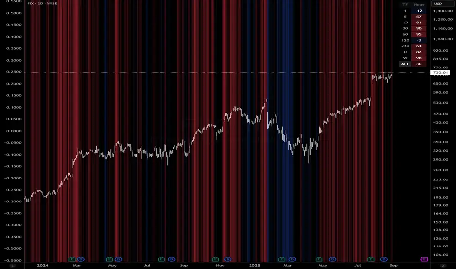
Kelly Position Size CalculatorThis position sizing calculator implements the Kelly Criterion, developed by John L. Kelly Jr. at Bell Laboratories in 1956, to determine mathematically optimal position sizes for maximizing long-term wealth growth. Unlike arbitrary position sizing methods, this tool provides a scientifically solution based on your strategy's actual performance statistics and incorporates modern refinements from over six decades of academic research.
The Kelly Criterion addresses a fundamental question in capital allocation: "What fraction of capital should be allocated to each opportunity to maximize growth while avoiding ruin?" This question has profound implications for financial markets, where traders and investors constantly face decisions about optimal capital allocation (Van Tharp, 2007).
Theoretical Foundation
The Kelly Criterion for binary outcomes is expressed as f* = (bp - q) / b, where f* represents the optimal fraction of capital to allocate, b denotes the risk-reward ratio, p indicates the probability of success, and q represents the probability of loss (Kelly, 1956). This formula maximizes the expected logarithm of wealth, ensuring maximum long-term growth rate while avoiding the risk of ruin.
The mathematical elegance of Kelly's approach lies in its derivation from information theory. Kelly's original work was motivated by Claude Shannon's information theory (Shannon, 1948), recognizing that maximizing the logarithm of wealth is equivalent to maximizing the rate of information transmission. This connection between information theory and wealth accumulation provides a deep theoretical foundation for optimal position sizing.
The logarithmic utility function underlying the Kelly Criterion naturally embodies several desirable properties for capital management. It exhibits decreasing marginal utility, penalizes large losses more severely than it rewards equivalent gains, and focuses on geometric rather than arithmetic mean returns, which is appropriate for compounding scenarios (Thorp, 2006).
Scientific Implementation
This calculator extends beyond basic Kelly implementation by incorporating state of the art refinements from academic research:
Parameter Uncertainty Adjustment: Following Michaud (1989), the implementation applies Bayesian shrinkage to account for parameter estimation error inherent in small sample sizes. The adjustment formula f_adjusted = f_kelly × confidence_factor + f_conservative × (1 - confidence_factor) addresses the overconfidence bias documented by Baker and McHale (2012), where the confidence factor increases with sample size and the conservative estimate equals 0.25 (quarter Kelly).
Sample Size Confidence: The reliability of Kelly calculations depends critically on sample size. Research by Browne and Whitt (1996) provides theoretical guidance on minimum sample requirements, suggesting that at least 30 independent observations are necessary for meaningful parameter estimates, with 100 or more trades providing reliable estimates for most trading strategies.
Universal Asset Compatibility: The calculator employs intelligent asset detection using TradingView's built-in symbol information, automatically adapting calculations for different asset classes without manual configuration.
ASSET SPECIFIC IMPLEMENTATION
Equity Markets: For stocks and ETFs, position sizing follows the calculation Shares = floor(Kelly Fraction × Account Size / Share Price). This straightforward approach reflects whole share constraints while accommodating fractional share trading capabilities.
Foreign Exchange Markets: Forex markets require lot-based calculations following Lot Size = Kelly Fraction × Account Size / (100,000 × Base Currency Value). The calculator automatically handles major currency pairs with appropriate pip value calculations, following industry standards described by Archer (2010).
Futures Markets: Futures position sizing accounts for leverage and margin requirements through Contracts = floor(Kelly Fraction × Account Size / Margin Requirement). The calculator estimates margin requirements as a percentage of contract notional value, with specific adjustments for micro-futures contracts that have smaller sizes and reduced margin requirements (Kaufman, 2013).
Index and Commodity Markets: These markets combine characteristics of both equity and futures markets. The calculator automatically detects whether instruments are cash-settled or futures-based, applying appropriate sizing methodologies with correct point value calculations.
Risk Management Integration
The calculator integrates sophisticated risk assessment through two primary modes:
Stop Loss Integration: When fixed stop-loss levels are defined, risk calculation follows Risk per Trade = Position Size × Stop Loss Distance. This ensures that the Kelly fraction accounts for actual risk exposure rather than theoretical maximum loss, with stop-loss distance measured in appropriate units for each asset class.
Strategy Drawdown Assessment: For discretionary exit strategies, risk estimation uses maximum historical drawdown through Risk per Trade = Position Value × (Maximum Drawdown / 100). This approach assumes that individual trade losses will not exceed the strategy's historical maximum drawdown, providing a reasonable estimate for strategies with well-defined risk characteristics.
Fractional Kelly Approaches
Pure Kelly sizing can produce substantial volatility, leading many practitioners to adopt fractional Kelly approaches. MacLean, Sanegre, Zhao, and Ziemba (2004) analyze the trade-offs between growth rate and volatility, demonstrating that half-Kelly typically reduces volatility by approximately 75% while sacrificing only 25% of the growth rate.
The calculator provides three primary Kelly modes to accommodate different risk preferences and experience levels. Full Kelly maximizes growth rate while accepting higher volatility, making it suitable for experienced practitioners with strong risk tolerance and robust capital bases. Half Kelly offers a balanced approach popular among professional traders, providing optimal risk-return balance by reducing volatility significantly while maintaining substantial growth potential. Quarter Kelly implements a conservative approach with low volatility, recommended for risk-averse traders or those new to Kelly methodology who prefer gradual introduction to optimal position sizing principles.
Empirical Validation and Performance
Extensive academic research supports the theoretical advantages of Kelly sizing. Hakansson and Ziemba (1995) provide a comprehensive review of Kelly applications in finance, documenting superior long-term performance across various market conditions and asset classes. Estrada (2008) analyzes Kelly performance in international equity markets, finding that Kelly-based strategies consistently outperform fixed position sizing approaches over extended periods across 19 developed markets over a 30-year period.
Several prominent investment firms have successfully implemented Kelly-based position sizing. Pabrai (2007) documents the application of Kelly principles at Berkshire Hathaway, noting Warren Buffett's concentrated portfolio approach aligns closely with Kelly optimal sizing for high-conviction investments. Quantitative hedge funds, including Renaissance Technologies and AQR, have incorporated Kelly-based risk management into their systematic trading strategies.
Practical Implementation Guidelines
Successful Kelly implementation requires systematic application with attention to several critical factors:
Parameter Estimation: Accurate parameter estimation represents the greatest challenge in practical Kelly implementation. Brown (1976) notes that small errors in probability estimates can lead to significant deviations from optimal performance. The calculator addresses this through Bayesian adjustments and confidence measures.
Sample Size Requirements: Users should begin with conservative fractional Kelly approaches until achieving sufficient historical data. Strategies with fewer than 30 trades may produce unreliable Kelly estimates, regardless of adjustments. Full confidence typically requires 100 or more independent trade observations.
Market Regime Considerations: Parameters that accurately describe historical performance may not reflect future market conditions. Ziemba (2003) recommends regular parameter updates and conservative adjustments when market conditions change significantly.
Professional Features and Customization
The calculator provides comprehensive customization options for professional applications:
Multiple Color Schemes: Eight professional color themes (Gold, EdgeTools, Behavioral, Quant, Ocean, Fire, Matrix, Arctic) with dark and light theme compatibility ensure optimal visibility across different trading environments.
Flexible Display Options: Adjustable table size and position accommodate various chart layouts and user preferences, while maintaining analytical depth and clarity.
Comprehensive Results: The results table presents essential information including asset specifications, strategy statistics, Kelly calculations, sample confidence measures, position values, risk assessments, and final position sizes in appropriate units for each asset class.
Limitations and Considerations
Like any analytical tool, the Kelly Criterion has important limitations that users must understand:
Stationarity Assumption: The Kelly Criterion assumes that historical strategy statistics represent future performance characteristics. Non-stationary market conditions may invalidate this assumption, as noted by Lo and MacKinlay (1999).
Independence Requirement: Each trade should be independent to avoid correlation effects. Many trading strategies exhibit serial correlation in returns, which can affect optimal position sizing and may require adjustments for portfolio applications.
Parameter Sensitivity: Kelly calculations are sensitive to parameter accuracy. Regular calibration and conservative approaches are essential when parameter uncertainty is high.
Transaction Costs: The implementation incorporates user-defined transaction costs but assumes these remain constant across different position sizes and market conditions, following Ziemba (2003).
Advanced Applications and Extensions
Multi-Asset Portfolio Considerations: While this calculator optimizes individual position sizes, portfolio-level applications require additional considerations for correlation effects and aggregate risk management. Simplified portfolio approaches include treating positions independently with correlation adjustments.
Behavioral Factors: Behavioral finance research reveals systematic biases that can interfere with Kelly implementation. Kahneman and Tversky (1979) document loss aversion, overconfidence, and other cognitive biases that lead traders to deviate from optimal strategies. Successful implementation requires disciplined adherence to calculated recommendations.
Time-Varying Parameters: Advanced implementations may incorporate time-varying parameter models that adjust Kelly recommendations based on changing market conditions, though these require sophisticated econometric techniques and substantial computational resources.
Comprehensive Usage Instructions and Practical Examples
Implementation begins with loading the calculator on your desired trading instrument's chart. The system automatically detects asset type across stocks, forex, futures, and cryptocurrency markets while extracting current price information. Navigation to the indicator settings allows input of your specific strategy parameters.
Strategy statistics configuration requires careful attention to several key metrics. The win rate should be calculated from your backtest results using the formula of winning trades divided by total trades multiplied by 100. Average win represents the sum of all profitable trades divided by the number of winning trades, while average loss calculates the sum of all losing trades divided by the number of losing trades, entered as a positive number. The total historical trades parameter requires the complete number of trades in your backtest, with a minimum of 30 trades recommended for basic functionality and 100 or more trades optimal for statistical reliability. Account size should reflect your available trading capital, specifically the risk capital allocated for trading rather than total net worth.
Risk management configuration adapts to your specific trading approach. The stop loss setting should be enabled if you employ fixed stop-loss exits, with the stop loss distance specified in appropriate units depending on the asset class. For stocks, this distance is measured in dollars, for forex in pips, and for futures in ticks. When stop losses are not used, the maximum strategy drawdown percentage from your backtest provides the risk assessment baseline. Kelly mode selection offers three primary approaches: Full Kelly for aggressive growth with higher volatility suitable for experienced practitioners, Half Kelly for balanced risk-return optimization popular among professional traders, and Quarter Kelly for conservative approaches with reduced volatility.
Display customization ensures optimal integration with your trading environment. Eight professional color themes provide optimization for different chart backgrounds and personal preferences. Table position selection allows optimal placement within your chart layout, while table size adjustment ensures readability across different screen resolutions and viewing preferences.
Detailed Practical Examples
Example 1: SPY Swing Trading Strategy
Consider a professionally developed swing trading strategy for SPY (S&P 500 ETF) with backtesting results spanning 166 total trades. The strategy achieved 110 winning trades, representing a 66.3% win rate, with an average winning trade of $2,200 and average losing trade of $862. The maximum drawdown reached 31.4% during the testing period, and the available trading capital amounts to $25,000. This strategy employs discretionary exits without fixed stop losses.
Implementation requires loading the calculator on the SPY daily chart and configuring the parameters accordingly. The win rate input receives 66.3, while average win and loss inputs receive 2200 and 862 respectively. Total historical trades input requires 166, with account size set to 25000. The stop loss function remains disabled due to the discretionary exit approach, with maximum strategy drawdown set to 31.4%. Half Kelly mode provides the optimal balance between growth and risk management for this application.
The calculator generates several key outputs for this scenario. The risk-reward ratio calculates automatically to 2.55, while the Kelly fraction reaches approximately 53% before scientific adjustments. Sample confidence achieves 100% given the 166 trades providing high statistical confidence. The recommended position settles at approximately 27% after Half Kelly and Bayesian adjustment factors. Position value reaches approximately $6,750, translating to 16 shares at a $420 SPY price. Risk per trade amounts to approximately $2,110, representing 31.4% of position value, with expected value per trade reaching approximately $1,466. This recommendation represents the mathematically optimal balance between growth potential and risk management for this specific strategy profile.
Example 2: EURUSD Day Trading with Stop Losses
A high-frequency EURUSD day trading strategy demonstrates different parameter requirements compared to swing trading approaches. This strategy encompasses 89 total trades with a 58% win rate, generating an average winning trade of $180 and average losing trade of $95. The maximum drawdown reached 12% during testing, with available capital of $10,000. The strategy employs fixed stop losses at 25 pips and take profit targets at 45 pips, providing clear risk-reward parameters.
Implementation begins with loading the calculator on the EURUSD 1-hour chart for appropriate timeframe alignment. Parameter configuration includes win rate at 58, average win at 180, and average loss at 95. Total historical trades input receives 89, with account size set to 10000. The stop loss function is enabled with distance set to 25 pips, reflecting the fixed exit strategy. Quarter Kelly mode provides conservative positioning due to the smaller sample size compared to the previous example.
Results demonstrate the impact of smaller sample sizes on Kelly calculations. The risk-reward ratio calculates to 1.89, while the Kelly fraction reaches approximately 32% before adjustments. Sample confidence achieves 89%, providing moderate statistical confidence given the 89 trades. The recommended position settles at approximately 7% after Quarter Kelly application and Bayesian shrinkage adjustment for the smaller sample. Position value amounts to approximately $700, translating to 0.07 standard lots. Risk per trade reaches approximately $175, calculated as 25 pips multiplied by lot size and pip value, with expected value per trade at approximately $49. This conservative position sizing reflects the smaller sample size, with position sizes expected to increase as trade count surpasses 100 and statistical confidence improves.
Example 3: ES1! Futures Systematic Strategy
Systematic futures trading presents unique considerations for Kelly criterion application, as demonstrated by an E-mini S&P 500 futures strategy encompassing 234 total trades. This systematic approach achieved a 45% win rate with an average winning trade of $1,850 and average losing trade of $720. The maximum drawdown reached 18% during the testing period, with available capital of $50,000. The strategy employs 15-tick stop losses with contract specifications of $50 per tick, providing precise risk control mechanisms.
Implementation involves loading the calculator on the ES1! 15-minute chart to align with the systematic trading timeframe. Parameter configuration includes win rate at 45, average win at 1850, and average loss at 720. Total historical trades receives 234, providing robust statistical foundation, with account size set to 50000. The stop loss function is enabled with distance set to 15 ticks, reflecting the systematic exit methodology. Half Kelly mode balances growth potential with appropriate risk management for futures trading.
Results illustrate how favorable risk-reward ratios can support meaningful position sizing despite lower win rates. The risk-reward ratio calculates to 2.57, while the Kelly fraction reaches approximately 16%, lower than previous examples due to the sub-50% win rate. Sample confidence achieves 100% given the 234 trades providing high statistical confidence. The recommended position settles at approximately 8% after Half Kelly adjustment. Estimated margin per contract amounts to approximately $2,500, resulting in a single contract allocation. Position value reaches approximately $2,500, with risk per trade at $750, calculated as 15 ticks multiplied by $50 per tick. Expected value per trade amounts to approximately $508. Despite the lower win rate, the favorable risk-reward ratio supports meaningful position sizing, with single contract allocation reflecting appropriate leverage management for futures trading.
Example 4: MES1! Micro-Futures for Smaller Accounts
Micro-futures contracts provide enhanced accessibility for smaller trading accounts while maintaining identical strategy characteristics. Using the same systematic strategy statistics from the previous example but with available capital of $15,000 and micro-futures specifications of $5 per tick with reduced margin requirements, the implementation demonstrates improved position sizing granularity.
Kelly calculations remain identical to the full-sized contract example, maintaining the same risk-reward dynamics and statistical foundations. However, estimated margin per contract reduces to approximately $250 for micro-contracts, enabling allocation of 4-5 micro-contracts. Position value reaches approximately $1,200, while risk per trade calculates to $75, derived from 15 ticks multiplied by $5 per tick. This granularity advantage provides better position size precision for smaller accounts, enabling more accurate Kelly implementation without requiring large capital commitments.
Example 5: Bitcoin Swing Trading
Cryptocurrency markets present unique challenges requiring modified Kelly application approaches. A Bitcoin swing trading strategy on BTCUSD encompasses 67 total trades with a 71% win rate, generating average winning trades of $3,200 and average losing trades of $1,400. Maximum drawdown reached 28% during testing, with available capital of $30,000. The strategy employs technical analysis for exits without fixed stop losses, relying on price action and momentum indicators.
Implementation requires conservative approaches due to cryptocurrency volatility characteristics. Quarter Kelly mode is recommended despite the high win rate to account for crypto market unpredictability. Expected position sizing remains reduced due to the limited sample size of 67 trades, requiring additional caution until statistical confidence improves. Regular parameter updates are strongly recommended due to cryptocurrency market evolution and changing volatility patterns that can significantly impact strategy performance characteristics.
Advanced Usage Scenarios
Portfolio position sizing requires sophisticated consideration when running multiple strategies simultaneously. Each strategy should have its Kelly fraction calculated independently to maintain mathematical integrity. However, correlation adjustments become necessary when strategies exhibit related performance patterns. Moderately correlated strategies should receive individual position size reductions of 10-20% to account for overlapping risk exposure. Aggregate portfolio risk monitoring ensures total exposure remains within acceptable limits across all active strategies. Professional practitioners often consider using lower fractional Kelly approaches, such as Quarter Kelly, when running multiple strategies simultaneously to provide additional safety margins.
Parameter sensitivity analysis forms a critical component of professional Kelly implementation. Regular validation procedures should include monthly parameter updates using rolling 100-trade windows to capture evolving market conditions while maintaining statistical relevance. Sensitivity testing involves varying win rates by ±5% and average win/loss ratios by ±10% to assess recommendation stability under different parameter assumptions. Out-of-sample validation reserves 20% of historical data for parameter verification, ensuring that optimization doesn't create curve-fitted results. Regime change detection monitors actual performance against expected metrics, triggering parameter reassessment when significant deviations occur.
Risk management integration requires professional overlay considerations beyond pure Kelly calculations. Daily loss limits should cease trading when daily losses exceed twice the calculated risk per trade, preventing emotional decision-making during adverse periods. Maximum position limits should never exceed 25% of account value in any single position regardless of Kelly recommendations, maintaining diversification principles. Correlation monitoring reduces position sizes when holding multiple correlated positions that move together during market stress. Volatility adjustments consider reducing position sizes during periods of elevated VIX above 25 for equity strategies, adapting to changing market conditions.
Troubleshooting and Optimization
Professional implementation often encounters specific challenges requiring systematic troubleshooting approaches. Zero position size displays typically result from insufficient capital for minimum position sizes, negative expected values, or extremely conservative Kelly calculations. Solutions include increasing account size, verifying strategy statistics for accuracy, considering Quarter Kelly mode for conservative approaches, or reassessing overall strategy viability when fundamental issues exist.
Extremely high Kelly fractions exceeding 50% usually indicate underlying problems with parameter estimation. Common causes include unrealistic win rates, inflated risk-reward ratios, or curve-fitted backtest results that don't reflect genuine trading conditions. Solutions require verifying backtest methodology, including all transaction costs in calculations, testing strategies on out-of-sample data, and using conservative fractional Kelly approaches until parameter reliability improves.
Low sample confidence below 50% reflects insufficient historical trades for reliable parameter estimation. This situation demands gathering additional trading data, using Quarter Kelly approaches until reaching 100 or more trades, applying extra conservatism in position sizing, and considering paper trading to build statistical foundations without capital risk.
Inconsistent results across similar strategies often stem from parameter estimation differences, market regime changes, or strategy degradation over time. Professional solutions include standardizing backtest methodology across all strategies, updating parameters regularly to reflect current conditions, and monitoring live performance against expectations to identify deteriorating strategies.
Position sizes that appear inappropriately large or small require careful validation against traditional risk management principles. Professional standards recommend never risking more than 2-3% per trade regardless of Kelly calculations. Calibration should begin with Quarter Kelly approaches, gradually increasing as comfort and confidence develop. Most institutional traders utilize 25-50% of full Kelly recommendations to balance growth with prudent risk management.
Market condition adjustments require dynamic approaches to Kelly implementation. Trending markets may support full Kelly recommendations when directional momentum provides favorable conditions. Ranging or volatile markets typically warrant reducing to Half or Quarter Kelly to account for increased uncertainty. High correlation periods demand reducing individual position sizes when multiple positions move together, concentrating risk exposure. News and event periods often justify temporary position size reductions during high-impact releases that can create unpredictable market movements.
Performance monitoring requires systematic protocols to ensure Kelly implementation remains effective over time. Weekly reviews should compare actual versus expected win rates and average win/loss ratios to identify parameter drift or strategy degradation. Position size efficiency and execution quality monitoring ensures that calculated recommendations translate effectively into actual trading results. Tracking correlation between calculated and realized risk helps identify discrepancies between theoretical and practical risk exposure.
Monthly calibration provides more comprehensive parameter assessment using the most recent 100 trades to maintain statistical relevance while capturing current market conditions. Kelly mode appropriateness requires reassessment based on recent market volatility and performance characteristics, potentially shifting between Full, Half, and Quarter Kelly approaches as conditions change. Transaction cost evaluation ensures that commission structures, spreads, and slippage estimates remain accurate and current.
Quarterly strategic reviews encompass comprehensive strategy performance analysis comparing long-term results against expectations and identifying trends in effectiveness. Market regime assessment evaluates parameter stability across different market conditions, determining whether strategy characteristics remain consistent or require fundamental adjustments. Strategic modifications to position sizing methodology may become necessary as markets evolve or trading approaches mature, ensuring that Kelly implementation continues supporting optimal capital allocation objectives.
Professional Applications
This calculator serves diverse professional applications across the financial industry. Quantitative hedge funds utilize the implementation for systematic position sizing within algorithmic trading frameworks, where mathematical precision and consistent application prove essential for institutional capital management. Professional discretionary traders benefit from optimized position management that removes emotional bias while maintaining flexibility for market-specific adjustments. Portfolio managers employ the calculator for developing risk-adjusted allocation strategies that enhance returns while maintaining prudent risk controls across diverse asset classes and investment strategies.
Individual traders seeking mathematical optimization of capital allocation find the calculator provides institutional-grade methodology previously available only to professional money managers. The Kelly Criterion establishes theoretical foundation for optimal capital allocation across both single strategies and multiple trading systems, offering significant advantages over arbitrary position sizing methods that rely on intuition or fixed percentage approaches. Professional implementation ensures consistent application of mathematically sound principles while adapting to changing market conditions and strategy performance characteristics.
Conclusion
The Kelly Criterion represents one of the few mathematically optimal solutions to fundamental investment problems. When properly understood and carefully implemented, it provides significant competitive advantage in financial markets. This calculator implements modern refinements to Kelly's original formula while maintaining accessibility for practical trading applications.
Success with Kelly requires ongoing learning, systematic application, and continuous refinement based on market feedback and evolving research. Users who master Kelly principles and implement them systematically can expect superior risk-adjusted returns and more consistent capital growth over extended periods.
The extensive academic literature provides rich resources for deeper study, while practical experience builds the intuition necessary for effective implementation. Regular parameter updates, conservative approaches with limited data, and disciplined adherence to calculated recommendations are essential for optimal results.
References
Archer, M. D. (2010). Getting Started in Currency Trading: Winning in Today's Forex Market (3rd ed.). John Wiley & Sons.
Baker, R. D., & McHale, I. G. (2012). An empirical Bayes approach to optimising betting strategies. Journal of the Royal Statistical Society: Series D (The Statistician), 61(1), 75-92.
Breiman, L. (1961). Optimal gambling systems for favorable games. In J. Neyman (Ed.), Proceedings of the Fourth Berkeley Symposium on Mathematical Statistics and Probability (pp. 65-78). University of California Press.
Brown, D. B. (1976). Optimal portfolio growth: Logarithmic utility and the Kelly criterion. In W. T. Ziemba & R. G. Vickson (Eds.), Stochastic Optimization Models in Finance (pp. 1-23). Academic Press.
Browne, S., & Whitt, W. (1996). Portfolio choice and the Bayesian Kelly criterion. Advances in Applied Probability, 28(4), 1145-1176.
Estrada, J. (2008). Geometric mean maximization: An overlooked portfolio approach? The Journal of Investing, 17(4), 134-147.
Hakansson, N. H., & Ziemba, W. T. (1995). Capital growth theory. In R. A. Jarrow, V. Maksimovic, & W. T. Ziemba (Eds.), Handbooks in Operations Research and Management Science (Vol. 9, pp. 65-86). Elsevier.
Kahneman, D., & Tversky, A. (1979). Prospect theory: An analysis of decision under risk. Econometrica, 47(2), 263-291.
Kaufman, P. J. (2013). Trading Systems and Methods (5th ed.). John Wiley & Sons.
Kelly Jr, J. L. (1956). A new interpretation of information rate. Bell System Technical Journal, 35(4), 917-926.
Lo, A. W., & MacKinlay, A. C. (1999). A Non-Random Walk Down Wall Street. Princeton University Press.
MacLean, L. C., Sanegre, E. O., Zhao, Y., & Ziemba, W. T. (2004). Capital growth with security. Journal of Economic Dynamics and Control, 28(4), 937-954.
MacLean, L. C., Thorp, E. O., & Ziemba, W. T. (2011). The Kelly Capital Growth Investment Criterion: Theory and Practice. World Scientific.
Michaud, R. O. (1989). The Markowitz optimization enigma: Is 'optimized' optimal? Financial Analysts Journal, 45(1), 31-42.
Pabrai, M. (2007). The Dhandho Investor: The Low-Risk Value Method to High Returns. John Wiley & Sons.
Shannon, C. E. (1948). A mathematical theory of communication. Bell System Technical Journal, 27(3), 379-423.
Tharp, V. K. (2007). Trade Your Way to Financial Freedom (2nd ed.). McGraw-Hill.
Thorp, E. O. (2006). The Kelly criterion in blackjack sports betting, and the stock market. In L. C. MacLean, E. O. Thorp, & W. T. Ziemba (Eds.), The Kelly Capital Growth Investment Criterion: Theory and Practice (pp. 789-832). World Scientific.
Van Tharp, K. (2007). Trade Your Way to Financial Freedom (2nd ed.). McGraw-Hill Education.
Vince, R. (1992). The Mathematics of Money Management: Risk Analysis Techniques for Traders. John Wiley & Sons.
Vince, R., & Zhu, H. (2015). Optimal betting under parameter uncertainty. Journal of Statistical Planning and Inference, 161, 19-31.
Ziemba, W. T. (2003). The Stochastic Programming Approach to Asset, Liability, and Wealth Management. The Research Foundation of AIMR.
Further Reading
For comprehensive understanding of Kelly Criterion applications and advanced implementations:
MacLean, L. C., Thorp, E. O., & Ziemba, W. T. (2011). The Kelly Capital Growth Investment Criterion: Theory and Practice. World Scientific.
Vince, R. (1992). The Mathematics of Money Management: Risk Analysis Techniques for Traders. John Wiley & Sons.
Thorp, E. O. (2017). A Man for All Markets: From Las Vegas to Wall Street. Random House.
Cover, T. M., & Thomas, J. A. (2006). Elements of Information Theory (2nd ed.). John Wiley & Sons.
Ziemba, W. T., & Vickson, R. G. (Eds.). (2006). Stochastic Optimization Models in Finance. World Scientific.

X σ mirrorX σ Mirror — Volatility Projection & Price Action Guide
The X σ Mirror is a volatility-mapping tool that measures the prior period’s trading range, then mirrors and projects that range onto the current period. Anchored from the current period’s opening price, the indicator divides this projected range into quartiles, creating a structured price map that adapts to the asset’s recent volatility profile.
Core Methodology
Range Measurement – At the close of each user-selected higher timeframe (daily, 4-hour, weekly, etc.), the indicator captures the prior period’s high, low, and midpoint (equilibrium). This defines the “volatility envelope” for the next period.
Projection from the Open – The full prior range is projected above and below the current period’s open. This symmetrical mirroring anchors the volatility measurement to a logical starting point for intraperiod price movement.
Quartile Breakdown – The projected range is segmented into precise increments: 0.25×, 0.50×, 0.75×, 1.0×, 1.25×, 1.5×, and 2.0× of the prior range. These serve as price “checkpoints” that reflect proportional expansions or contractions relative to historical volatility.
How It Guides Price Action
Dynamic Support & Resistance – Quartile levels often act as temporary barriers or accelerators for price movement, highlighting areas where order flow may cluster.
Momentum Tracking – Price acceptance above successive quartiles suggests sustained directional strength, while repeated failures to breach a quartile indicate exhaustion.
Risk Management – The mirrored range and quartile levels help traders size positions, define stop placements, and set profit targets with volatility-adjusted precision.
Market Context – By anchoring the projection from the open, the indicator aligns volatility expectations with the session’s actual market structure, rather than static fixed levels.
Application
The X σ Mirror is adaptable across assets and timeframes, making it suitable for intraday traders tracking the unfolding session, as well as swing traders monitoring multi-day expansion potential. By combining historical range analysis with real-time market positioning, it provides a balanced framework for anticipating price behavior within a probabilistic structure.

ATR+CCI Monetary Risk Tool - TP/SL⚙️ ATR+CCI Monetary Risk Tool — Volatility-aware TP/SL & Position Sizing
Exact prices (no rounding), ATR-percentile dynamic stops, and risk-budget sizing for consistent execution.
🧠 What this indicator is
A risk-first planning tool. It doesn’t generate orders; it gives you clean, objective levels (Entry, SL, TP) and position size derived from your risk budget. It shows only the latest setup to keep charts readable, and a compact on-chart table summarizing the numbers you actually act on.
✨ What makes it different
Dynamic SL by regime (ATR percentile): Instead of a fixed multiple, the SL multiplier adapts to the current volatility percentile (low / medium / high). That helps avoid tight stops in noisy markets and over-wide stops in quiet markets.
Risk budgeting, not guesswork: Size is computed from Account Balance × Max Risk % divided by SL distance × point value. You risk the same dollars across assets/timeframes.
Precision that matches your instrument: Entry, TP, SL, and SL Distance are displayed as exact prices (no rounding), truncated to syminfo.mintick so they align with broker/exchange precision.
Symbol-aware point value: Uses syminfo.pointvalue so you don’t maintain tick tables.
Non-repaint option: Work from closed bars to keep the plan stable.
🔧 How to use (quick start)
Add to chart and pick your timeframe and symbol.
In settings:
Set Account Balance (USD) and Max Risk per Trade (%).
Choose R:R (1:1 … 1:5).
Pick ATR Period and CCI Period (defaults are sensible).
Keep Dynamic ATR ON to adapt SL by regime.
Keep Use closed-bar values ON to avoid repaint when planning.
Read the labels (Entry/TP/SL) and the table (SL Distance, Position Size, Max USD Risk, ATR Percentile, effective SL Mult).
Combine with your entry trigger (price action, levels, momentum, etc.). This indicator handles risk & targets.
📐 How levels are computed
Bias: CCI ≥ 0 ⇒ long, otherwise short.
ATR Percentile: Percent rank of ATR(atrPeriod) over a lookback window.
Effective SL Mult:
If percentile < Low threshold ⇒ use Low SL Mult (tighter).
If between thresholds ⇒ use Base SL Mult.
If percentile > High threshold ⇒ use High SL Mult (wider).
Stop-Loss: SL = Entry ± ATR × SL_Mult (minus for long, plus for short).
Take-Profit: TP = Entry ± (Entry − SL) × R (R from the R:R dropdown).
Position Size:
USD Risk = Balance × Risk%
Contracts = USD Risk ÷ (|Entry − SL| × PointValue)
For futures, quantity is floored to whole contracts.
Exact prices: Entry/TP/SL and SL Distance are not rounded; they’re truncated to mintick so what you see matches valid price increments.
📊 What you’ll see on chart
Latest Entry (blue), TP (green), SL (red) with labels (optional emojis: ➡️ 🎯 🛑).
Info Table with:
Bias, Entry, TP, SL (exact, truncated to mintick)
SL Distance (exact, truncated)
Position Size (contracts/units)
Max USD Risk
Point Value
ATR Percentile and effective SL Mult
🧪 Practical examples
High-volatility session (e.g., XAUUSD, 1H): ATR percentile is high ⇒ wider SL, smaller size. Reduces churn from normal noise during macro events.
Range-bound market (e.g., EURUSD, 4H): ATR percentile low ⇒ tighter SL, better R:R. Helps you avoid carrying unnecessary risk.
Index swing planning (e.g., ES1!, Daily): Non-repaint levels + risk budgeting = consistent sizing across days/weeks, easier to review and journal.
🧭 Why traders should use it
Consistency: Same dollar risk regardless of instrument or volatility regime.
Clarity: One-trade view forces focus; you see the numbers that matter.
Adaptivity: Stops calibrated to the market’s current behavior, not last month’s.
Discipline: A visible checklist (SL distance, size, USD risk) before you hit buy/sell.
🔧 Input guide (practical defaults)
CCI Period: 100 by default; use as a bias filter, not an entry signal.
ATR Period: 14 by default; raise for smoother, lower for more reactive.
ATR Percentile Lookback: 200 by default (stable regime detection).
Percentile thresholds: 33/66 by default; widen the gap to change how often regimes switch.
SL Mults: Start ~1.5 / 2.0 / 2.5 (low/base/high). Tune by asset.
Risk % per trade: Common pro ranges are 0.25–1.0%; adjust to your risk tolerance.
R:R: Start with 1:2 or 1:3 for balanced skew; adapt to strategy edge.
Closed-bar values: Keep ON for planning/live; turn OFF only for exploration.
💡 Best practices
Combine with your entry logic (structure, momentum, liquidity levels).
Review ATR percentile and effective SL Mult across sessions so you understand regime shifts.
For futures, remember size is floored to whole contracts—safer by design.
Journal trades with the table snapshot to improve risk discipline over time.
⚠️ Notes & limitations
This is not a strategy; it does not place orders or alerts.
No slippage/commissions modeled here; build a strategy() version for backtests that mirror your broker/exchange.
Displayed non-price metrics use two decimals; prices and SL Distance are exact (truncated to mintick).
📎 Disclaimer
For educational purposes only. Not financial advice. Markets involve risk. Test thoroughly before trading live.
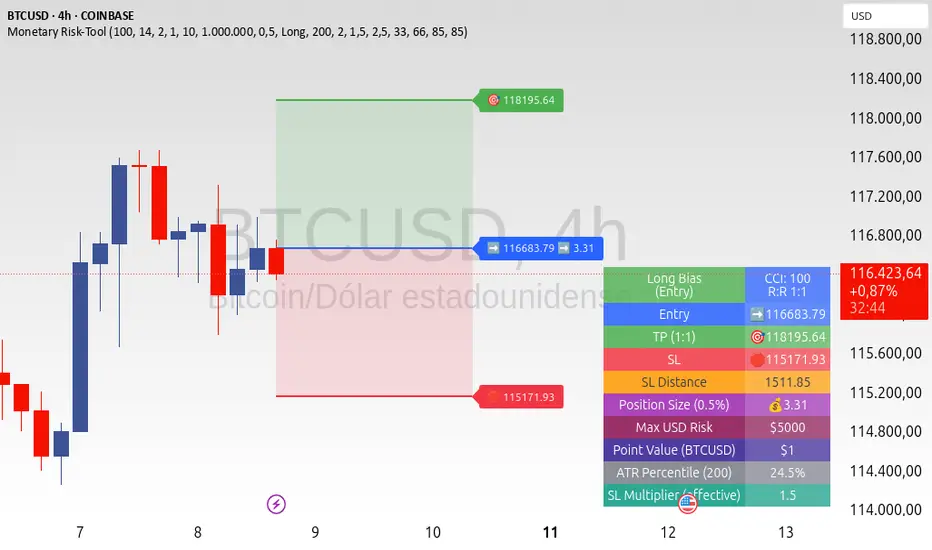
Harmonic BloomHarmonic Bloom - Advanced Geometric Analysis
Building upon my previous Fibonacci inspired indicator "TrendZone", Harmonic Bloom is a sophisticated geometric trading indicator inspired by W.D. Gann's legendary market geometry principles. It reveals market structure through three key pivot points and dynamic angular analysis, creating powerful harmonic intersections for precision trading.
🎯 Core Features:
📍 Three-Point Gann System:
Set 3 custom pivot points to define your analysis timeframe
Automatic trend detection (bullish/bearish) between pivots
Dynamic geometric box construction following Gann's square principles
📐 Gann-Style 45° Angle Projections:
Pivot 2 Line: Follows trend direction (up if bullish, down if bearish)
Pivot 3 Line: Creates opposition (opposite direction to Pivot 2)
Corner Line: Mirrors Pivot 2 from appropriate box corner
All angles project forward using Gann's 1x1 (45°) methodology for future price targets
⚡ POWER OF HARMONIC INTERSECTIONS:
Confluence Zones: Where multiple 45° angles intersect create the strongest support/resistance
Geometric Harmony: Intersections represent natural market turning points
Time-Price Balance: Following Gann's principle that time and price must be in harmony
Multiple Timeframe Resonance: Intersection points often align across different timeframes
High-Probability Reversals: Markets frequently respect these geometric intersection levels
📊 Customizable Retracement Levels:
8 fully configurable levels (default: 0.0, 0.25, 0.5, 0.75, 1.0, 1.25, 1.5, 1.75)
Choose between 25% or 50% trendline alignment
Individual style controls for each level
🔢 Advanced Gann Analytics:
Fibonacci sequence detection in bar counts (Gann studied natural number sequences)
Numerology sum analysis on pivot prices (Gann's mystical number approach)
Special highlighting for significant numbers
Optional on-chart labels for key metrics
📈 Trading Applications:
✅ Support/Resistance: Use retracement levels for entry/exit points
✅ Gann Angles: 45° lines show momentum direction and strength following Gann's time-price theory
✅ Intersection Trading: Most powerful signals occur at harmonic intersections where multiple angles converge
✅ Price Targets: Forward projections provide future price objectives using Gann's geometric principles
✅ Market Geometry: Identify harmonic patterns and geometric confluences
✅ Time Analysis: Fibonacci-based bar counting for timing decisions (Gann emphasized time cycles)
🌟 Why Harmonic Intersections Are So Powerful:
Gann believed that markets move in geometric harmony, and when multiple angles intersect, they create "magnetic price levels" where:
Maximum Energy Convergence: Multiple geometric forces meet at one point
Natural Turning Points: Markets respect these intersections as natural support/resistance
Time-Price Synchronicity: Intersections often coincide with significant time cycles
Multi-Dimensional Confirmation: Price, time, and geometry align simultaneously
⚙️ Highly Customizable:
All colors, widths, and styles adjustable
Toggle any feature on/off independently
Extend projections beyond the analysis box
Choose your preferred visual presentation
Perfect for traders who use Gann theory, geometric analysis, harmonic patterns, and mathematical market structure. The true power lies in trading the intersection points where multiple harmonic angles converge - these represent the market's most significant geometric turning points.

Smart MTF S/R Levels[BullByte]
Smart MTF S/R Levels
Introduction & Motivation
Support and Resistance (S/R) levels are the backbone of technical analysis. However, most traders face two major challenges:
Manual S/R Marking: Drawing S/R levels by hand is time-consuming, subjective, and often inconsistent.
Multi-Timeframe Blind Spots: Key S/R levels from higher or lower timeframes are often missed, leading to surprise reversals or missed opportunities.
Smart MTF S/R Levels was created to solve these problems. It is a fully automated, multi-timeframe, multi-method S/R detection and visualization tool, designed to give traders a complete, objective, and actionable view of the market’s most important price zones.
What Makes This Indicator Unique?
Multi-Timeframe Analysis: Simultaneously analyzes up to three user-selected timeframes, ensuring you never miss a critical S/R level from any timeframe.
Multi-Method Confluence: Integrates several respected S/R detection methods—Swings, Pivots, Fibonacci, Order Blocks, and Volume Profile—into a single, unified system.
Zone Clustering: Automatically merges nearby levels into “zones” to reduce clutter and highlight areas of true market consensus.
Confluence Scoring: Each zone is scored by the number of methods and timeframes in agreement, helping you instantly spot the most significant S/R areas.
Reaction Counting: Tracks how many times price has recently interacted with each zone, providing a real-world measure of its importance.
Customizable Dashboard: A real-time, on-chart table summarizes all key S/R zones, their origins, confluence, and proximity to price.
Smart Alerts: Get notified when price approaches high-confluence zones, so you never miss a critical trading opportunity.
Why Should a Trader Use This?
Objectivity: Removes subjectivity from S/R analysis by using algorithmic detection and clustering.
Efficiency: Saves hours of manual charting and reduces analysis fatigue.
Comprehensiveness: Ensures you are always aware of the most relevant S/R zones, regardless of your trading timeframe.
Actionability: The dashboard and alerts make it easy to act on the most important levels, improving trade timing and risk management.
Adaptability: Works for all asset classes (stocks, forex, crypto, futures) and all trading styles (scalping, swing, position).
The Gap This Indicator Fills
Most S/R indicators focus on a single method or timeframe, leading to incomplete analysis. Manual S/R marking is error-prone and inconsistent. This indicator fills the gap by:
Automating S/R detection across multiple timeframes and methods
Objectively scoring and ranking zones by confluence and reaction
Presenting all this information in a clear, actionable dashboard
How Does It Work? (Technical Logic)
1. Level Detection
For each selected timeframe, the script detects S/R levels using:
SW (Swing High/Low): Recent price pivots where reversals occurred.
Pivot: Classic floor trader pivots (P, S1, R1).
Fib (Fibonacci): Key retracement levels (0.236, 0.382, 0.5, 0.618, 0.786) over the last 50 bars.
Bull OB / Bear OB: Institutional price zones based on bullish/bearish engulfing patterns.
VWAP / POC: Volume Weighted Average Price and Point of Control over the last 50 bars.
2. Level Clustering
Levels within a user-defined % distance are merged into a single “zone.”
Each zone records which methods and timeframes contributed to it.
3. Confluence & Reaction Scoring
Confluence: The number of unique methods/timeframes in agreement for a zone.
Reactions: The number of times price has touched or reversed at the zone in the recent past (user-defined lookback).
4. Filtering & Sorting
Only zones within a user-defined % of the current price are shown (to focus on actionable areas).
Zones can be sorted by confluence, reaction count, or proximity to price.
5. Visualization
Zones: Shaded boxes on the chart (green for support, red for resistance, blue for mixed).
Lines: Mark the exact level of each zone.
Labels: Show level, methods by timeframe (e.g., 15m (3 SW), 30m (1 VWAP)), and (if applicable) Fibonacci ratios.
Dashboard Table: Lists all nearby zones with full details.
6. Alerts
Optional alerts trigger when price approaches a zone with confluence above a user-set threshold.
Inputs & Customization (Explained for All Users)
Show Timeframe 1/2/3: Enable/disable analysis for each timeframe (e.g., 15m, 30m, 1h).
Show Swings/Pivots/Fibonacci/Order Blocks/Volume Profile: Select which S/R methods to include.
Show levels within X% of price: Only display zones near the current price (default: 3%).
How many swing highs/lows to show: Number of recent swings to include (default: 3).
Cluster levels within X%: Merge levels close together into a single zone (default: 0.25%).
Show Top N Zones: Limit the number of zones displayed (default: 8).
Bars to check for reactions: How far back to count price reactions (default: 100).
Sort Zones By: Choose how to rank zones in the dashboard (Confluence, Reactions, Distance).
Alert if Confluence >=: Set the minimum confluence score for alerts (default: 3).
Zone Box Width/Line Length/Label Offset: Control the appearance of zones and labels.
Dashboard Size/Location: Customize the dashboard table.
How to Read the Output
Shaded Boxes: Represent S/R zones. The color indicates type (green = support, red = resistance, blue = mixed).
Lines: Mark the precise level of each zone.
Labels: Show the level, methods by timeframe (e.g., 15m (3 SW), 30m (1 VWAP)), and (if applicable) Fibonacci ratios.
Dashboard Table: Columns include:
Level: Price of the zone
Methods (by TF): Which S/R methods and how many, per timeframe (see abbreviation key below)
Type: Support, Resistance, or Mixed
Confl.: Confluence score (higher = more significant)
React.: Number of recent price reactions
Dist %: Distance from current price (in %)
Abbreviations Used
SW = Swing High/Low (recent price pivots where reversals occurred)
Fib = Fibonacci Level (key retracement levels such as 0.236, 0.382, 0.5, 0.618, 0.786)
VWAP = Volume Weighted Average Price (price level weighted by volume)
POC = Point of Control (price level with the highest traded volume)
Bull OB = Bullish Order Block (institutional support zone from bullish price action)
Bear OB = Bearish Order Block (institutional resistance zone from bearish price action)
Pivot = Pivot Point (classic floor trader pivots: P, S1, R1)
These abbreviations appear in the dashboard and chart labels for clarity.
Example: How to Read the Dashboard and Labels (from the chart above)
Suppose you are trading BTCUSDT on a 15-minute chart. The dashboard at the top right shows several S/R zones, each with a breakdown of which timeframes and methods contributed to their detection:
Resistance zone at 119257.11:
The dashboard shows:
5m (1 SW), 15m (2 SW), 1h (3 SW)
This means the level 119257.11 was identified as a resistance zone by one swing high (SW) on the 5-minute timeframe, two swing highs on the 15-minute timeframe, and three swing highs on the 1-hour timeframe. The confluence score is 6 (total number of method/timeframe hits), and there has been 1 recent price reaction at this level. This suggests 119257.11 is a strong resistance zone, confirmed by multiple swing highs across all selected timeframes.
Mixed zone at 118767.97:
The dashboard shows:
5m (2 SW), 15m (2 SW)
This means the level 118767.97 was identified by two swing points on both the 5-minute and 15-minute timeframes. The confluence score is 4, and there have been 19 recent price reactions at this level, indicating it is a highly reactive zone.
Support zone at 117411.35:
The dashboard shows:
5m (2 SW), 1h (2 SW)
This means the level 117411.35 was identified as a support zone by two swing lows on the 5-minute timeframe and two swing lows on the 1-hour timeframe. The confluence score is 4, and there have been 2 recent price reactions at this level.
Mixed zone at 118291.45:
The dashboard shows:
15m (1 SW, 1 VWAP), 5m (1 VWAP), 1h (1 VWAP)
This means the level 118291.45 was identified by a swing and VWAP on the 15-minute timeframe, and by VWAP on both the 5-minute and 1-hour timeframes. The confluence score is 4, and there have been 12 recent price reactions at this level.
Support zone at 117103.10:
The dashboard shows:
15m (1 SW), 1h (1 SW)
This means the level 117103.10 was identified by a single swing low on both the 15-minute and 1-hour timeframes. The confluence score is 2, and there have been no recent price reactions at this level.
Resistance zone at 117899.33:
The dashboard shows:
5m (1 SW)
This means the level 117899.33 was identified by a single swing high on the 5-minute timeframe. The confluence score is 1, and there have been no recent price reactions at this level.
How to use this:
Zones with higher confluence (more methods and timeframes in agreement) and more recent reactions are generally more significant. For example, the resistance at 119257.11 is much stronger than the resistance at 117899.33, and the mixed zone at 118767.97 has shown the most recent price reactions, making it a key area to watch for potential reversals or breakouts.
Tip:
“SW” stands for Swing High/Low, and “VWAP” stands for Volume Weighted Average Price.
The format 15m (2 SW) means two swing points were detected on the 15-minute timeframe.
Best Practices & Recommendations
Use with Other Tools: This indicator is most powerful when combined with your own price action analysis and risk management.
Adjust Settings: Experiment with timeframes, clustering, and methods to suit your trading style and the asset’s volatility.
Watch for High Confluence: Zones with higher confluence and more reactions are generally more significant.
Limitations
No Future Prediction: The indicator does not predict future price movement; it highlights areas where price is statistically more likely to react.
Not a Standalone System: Should be used as part of a broader trading plan.
Historical Data: Reaction counts are based on historical price action and may not always repeat.
Disclaimer
This indicator is a technical analysis tool and does not constitute financial advice or a recommendation to buy or sell any asset. Trading involves risk, and past performance is not indicative of future results. Always use proper risk management and consult a financial advisor if needed.

[Top] LHAMA Consolidation DetectorIntroducing the Low-High Adaptive Moving Average (LHAMA 🦙), a powerful tool designed to help traders visually distinguish between trending and consolidating market phases. Unlike traditional moving averages that can produce false signals in choppy markets, the LHAMA is engineered to flatten out during periods of consolidation and become more responsive when a clear trend emerges.
This indicator's primary function is to act as a "Consolidation Detector." When the LHAMA line goes flat and adopts its "Flat Color," it serves as a clear visual cue that the market is range-bound. Conversely, when the line begins to slope and changes to its Bullish or Bearish color, it signals a potential breakout or the start of a new trend.
How It Works
The LHAMA is a type of adaptive moving average. Its adaptiveness is derived from a unique calculation that measures market "trendiness." It does this by tracking whether new highs or new lows are being made within a specified lookback period.
In a Trending Market: When the price consistently makes new highs or lows, the indicator's responsiveness increases, causing the LHAMA to track the price much more closely and responsively.
In a Consolidating Market: When the price is range-bound and fails to make new highs or lows, the responsiveness decreases significantly. This causes the LHAMA to flatten out and become less sensitive to minor price fluctuations, effectively filtering out market noise.
Key Features
Adaptive Calculation: The core engine of the indicator, which automatically adjusts its smoothing based on trend strength.
Slope-Based Coloring: The line's color dynamically changes based on its slope, providing an at-a-glance view of market conditions: bullish, bearish, or flat.
Multi-Line & Multi-Timeframe (MTF): You can enable up to six fully customizable LHAMA lines. Each line can be configured with its own length, colors, and can even be set to a different timeframe, allowing for comprehensive multi-timeframe analysis on a single chart.
Volatility Clouds: Each LHAMA can display an optional cloud around it. The cloud's width is based on your choice of either the Average True Range (ATR) or Standard Deviation (StdDev), offering a visual representation of volatility.
Volume Weighting: An option to incorporate volume into the adaptive calculation, making the LHAMA even more responsive during high-volume price movements.
How to Use
Identify Consolidation: The primary use case. A flat and consistently colored LHAMA line is a strong indication of a sideways or consolidating market. This can help traders avoid taking trend-following trades in choppy conditions.
Confirm Trends: When the LHAMA begins to slope upwards or downwards and changes to its trend color, it can be used to confirm the direction and strength of a new trend. The steeper the slope, the stronger the momentum, and more solid the directional color.
Dynamic Support & Resistance: Like other moving averages, the LHAMA can act as a dynamic level of support in an uptrend or resistance in a downtrend. The optional cloud can further define these zones.
Multi-MA Ribbon Strategy: By enabling multiple LHAMAs with different lengths (e.g., Fibonacci sequence like 14, 21, 34, 55), you can create a ribbon. The expansion of the ribbon indicates a strong trend, while its contraction signals a weakening trend or consolidation.
Settings Explained
Enable 🦙 Line: A simple checkbox to turn each of the six LHAMA lines on or off.
Length: The lookback period for the LHAMA calculation. Shorter lengths are more responsive, while longer lengths are smoother.
Timeframe: Set a specific timeframe for each LHAMA. Leave blank to use the chart's current timeframe.
Volume Weight: If checked, adds volume weighting to make the LHAMA more responsive to high-volume moves.
Colors (Bullish, Bearish, Flat): Customize the colors for each market state. To only see the line during consolidation, set the Bullish and Bearish colors to 100% transparency. To hide the line during consolidation, set the Flat color to 100% transparency.
Color Sensitivity: This is a crucial setting. Because price scales (tick sizes) vary widely between symbols, this setting allows you to adjust the sensitivity of the slope detection. A lower value requires a steeper slope to trigger a trend color, while a higher value is more sensitive.
Recommended settings are provided in the input tooltip as a starting point:
$5 Tick: 0.25 Sensitivity
$1 Tick: 0.75 Sensitivity
$0.25 Tick: 3 Sensitivity
$0.01 Tick: 50 Sensitivity
$0.005 Tick: 100 Sensitivity
Cloud Settings:
Show Cloud: Toggles the visibility of the volatility cloud around the LHAMA.
Width Based On: Choose between "ATR" or "StdDev" to calculate the cloud's width.
Cloud Length & Width: Set the lookback period and multiplier for the ATR/StdDev calculation to control the size of the cloud.
Position Size Calculator with Fees# Position Size Calculator with Portfolio Management - Manual
## Overview
The Position Size Calculator with Portfolio Management is an advanced Pine Script indicator designed to help traders calculate optimal position sizes based on their total portfolio value and risk management strategy. This tool automatically calculates your risk amount based on portfolio allocation percentages and determines the exact position size needed while accounting for trading fees.
## Key Features
- **Portfolio-Based Risk Management**: Calculates risk based on total portfolio value
- **Tiered Risk Allocation**: Separates trading allocation from total portfolio
- **Automatic Trade Direction Detection**: Determines long/short based on entry vs stop loss
- **Fee Integration**: Accounts for trading fees in position size calculations
- **Risk Factor Adjustment**: Allows scaling of position size up or down
- **Visual Display**: Shows all calculations in a clear, color-coded table
- **Automatic Risk Calculation**: No need to manually input risk amount
## Input Parameters
### Total Portfolio ($)
- **Purpose**: The total value of your investment portfolio
- **Default**: 0.0
- **Range**: Any positive value
- **Step**: 0.01
- **Example**: If your total portfolio is worth $100,000, enter 100000
### Trading Portfolio Allocation (%)
- **Purpose**: The percentage of your total portfolio allocated to active trading
- **Default**: 20.0%
- **Range**: 0.0% to 100.0%
- **Step**: 0.01
- **Example**: If you allocate 20% of your portfolio to trading, enter 20
### Risk from Trading (%)
- **Purpose**: The percentage of your trading allocation you're willing to risk per trade
- **Default**: 0.1%
- **Range**: Any positive value
- **Step**: 0.01
- **Example**: If you risk 0.1% of your trading allocation per trade, enter 0.1
### Entry Price ($)
- **Purpose**: The price at which you plan to enter the trade
- **Default**: 0.0
- **Range**: Any positive value
- **Step**: 0.01
### Stop Loss ($)
- **Purpose**: The price at which you will exit if the trade goes against you
- **Default**: 0.0
- **Range**: Any positive value
- **Step**: 0.01
### Risk Factor
- **Purpose**: A multiplier to scale your position size up or down
- **Default**: 1.0 (no scaling)
- **Range**: 0.0 to 10.0
- **Step**: 0.1
- **Examples**:
- 1.0 = Normal position size
- 2.0 = Double the position size
- 0.5 = Half the position size
### Fee (%)
- **Purpose**: The percentage fee charged per transaction
- **Default**: 0.01% (0.01)
- **Range**: 0.0% to 1.0%
- **Step**: 0.001
## How Risk Amount is Calculated
The script automatically calculates your risk amount using this formula:
```
Risk Amount = Total Portfolio × Trading Allocation (%) × Risk % ÷ 10,000
```
### Example Calculation:
- Total Portfolio: $100,000
- Trading Allocation: 20%
- Risk per Trade: 0.1%
**Risk Amount = $100,000 × 20 × 0.1 ÷ 10,000 = $20**
This means you would risk $20 per trade, which is 0.1% of your $20,000 trading allocation.
## Portfolio Structure Example
Let's say you have a $100,000 portfolio:
### Allocation Structure:
- **Total Portfolio**: $100,000
- **Trading Allocation (20%)**: $20,000
- **Long-term Investments (80%)**: $80,000
### Risk Management:
- **Risk per Trade (0.1% of trading)**: $20
- **Maximum trades at risk**: Could theoretically have 1,000 trades before risking entire trading allocation
## How Position Size is Calculated
### Trade Direction Detection
- **Long Trade**: Entry price > Stop loss price
- **Short Trade**: Entry price < Stop loss price
### Position Size Formulas
#### For Long Trades:
```
Position Size = -Risk Factor × Risk Amount / (Stop Loss × (1 - Fee) - Entry Price × (1 + Fee))
```
#### For Short Trades:
```
Position Size = -Risk Factor × Risk Amount / (Entry Price × (1 - Fee) - Stop Loss × (1 + Fee))
```
## Output Display
The indicator displays a comprehensive table with color-coded sections:
### Portfolio Information (Light Blue Background)
- **Portfolio (USD)**: Your total portfolio value
- **Trading Portfolio Allocation (%)**: Percentage allocated to trading
- **Risk as % of Trading**: Risk percentage per trade
### Trade Setup (Gray Background)
- **Entry Price**: Your specified entry price
- **Stop Loss**: Your specified stop loss price
- **Fee (%)**: Trading fee percentage
- **Risk Factor**: Position size multiplier
### Risk Analysis (Red Background)
- **Risk Amount**: Automatically calculated dollar risk
- **Effective Entry**: Actual entry cost including fees
- **Effective Exit**: Actual exit value including fees
- **Expected Loss**: Calculated loss if stop loss is hit
- **Deviation from Risk %**: Accuracy of risk calculation
### Final Result (Blue Background)
- **Position Size**: Number of shares/units to trade
## Usage Examples
### Example 1: Conservative Long Trade
- **Total Portfolio**: $50,000
- **Trading Allocation**: 15%
- **Risk per Trade**: 0.05%
- **Entry Price**: $25.00
- **Stop Loss**: $24.00
- **Risk Factor**: 1.0
- **Fee**: 0.01%
**Calculated Risk Amount**: $50,000 × 15% × 0.05% ÷ 100 = $3.75
### Example 2: Aggressive Short Trade
- **Total Portfolio**: $200,000
- **Trading Allocation**: 30%
- **Risk per Trade**: 0.2%
- **Entry Price**: $150.00
- **Stop Loss**: $155.00
- **Risk Factor**: 2.0
- **Fee**: 0.01%
**Calculated Risk Amount**: $200,000 × 30% × 0.2% ÷ 100 = $120
**Actual Risk**: $120 × 2.0 = $240 (due to risk factor)
## Color Coding System
- **Green/Red Header**: Trade direction (Long/Short)
- **Light Blue**: Portfolio management parameters
- **Gray**: Trade setup parameters
- **Red**: Risk-related calculations and results
- **Blue**: Final position size result
## Best Practices
### Portfolio Management
1. **Keep trading allocation reasonable** (typically 10-30% of total portfolio)
2. **Use conservative risk percentages** (0.05-0.2% per trade)
3. **Don't risk more than you can afford to lose**
### Risk Management
1. **Start with small risk factors** (1.0 or less) until comfortable
2. **Monitor your total exposure** across all open positions
3. **Adjust risk based on market conditions**
### Trade Execution
1. **Always validate calculations** before placing trades
2. **Account for slippage** in volatile markets
3. **Consider position size relative to liquidity**
## Risk Management Guidelines
### Conservative Approach
- Trading Allocation: 10-20%
- Risk per Trade: 0.05-0.1%
- Risk Factor: 0.5-1.0
### Moderate Approach
- Trading Allocation: 20-30%
- Risk per Trade: 0.1-0.15%
- Risk Factor: 1.0-1.5
### Aggressive Approach
- Trading Allocation: 30-40%
- Risk per Trade: 0.15-0.25%
- Risk Factor: 1.5-2.0
## Troubleshooting
### Common Issues
1. **Position Size shows 0**
- Verify all portfolio inputs are greater than 0
- Check that entry price differs from stop loss
- Ensure calculated risk amount is positive
2. **Very small position sizes**
- Increase risk percentage or risk factor
- Check if your risk amount is too small for the price difference
3. **Large risk deviation**
- Normal for very small positions
- Consider adjusting entry/stop loss levels
### Validation Checklist
- Total portfolio value is realistic
- Trading allocation percentage makes sense
- Risk percentage is conservative
- Entry and stop loss prices are valid
- Trade direction matches your intention
## Advanced Features
### Risk Factor Usage
- **Scaling up**: Use risk factors > 1.0 for high-confidence trades
- **Scaling down**: Use risk factors < 1.0 for uncertain trades
- **Never exceed**: Risk factors that would risk more than your comfort level
### Multiple Timeframe Analysis
- Use different risk factors for different timeframes
- Consider correlation between positions
- Adjust trading allocation based on market conditions
## Disclaimer
This tool is for educational and planning purposes only. Always verify calculations manually and consider market conditions, liquidity, and correlation between positions. The automated risk calculation assumes you're comfortable with the mathematical relationship between portfolio allocation and individual trade risk. Past performance doesn't guarantee future results, and all trading involves risk of loss.

Boomerang Trading Indicator# Boomerang News Trading Indicator
## Overview
The Boomerang Trading Indicator is designed to identify potential reversal opportunities following major economic news releases. This indicator analyzes the initial market reaction to news events and provides visual cues for potential counter-trend trading opportunities based on Fibonacci retracement levels.
## How It Works
### News Event Detection
- Automatically detects major news release times (NFP, CPI, FOMC, etc.)
- Analyzes the first significant price movement following news releases
- Requires minimum candle size threshold to filter out weak reactions
### First Move Analysis
The indicator employs multiple analytical methods to determine the initial market direction:
**Simple Analysis (High Confidence):**
- When the news candle has ≥70% body-to-total ratio, uses straightforward bullish/bearish classification
**Advanced Analysis (Complex Cases):**
- Volume-weighted direction analysis
- Momentum and wick pattern analysis
- Market structure and gap analysis
- Weighted voting system combining all methods
### Entry Signal Generation
Based on the "boomerang" concept where markets often reverse after initial news reactions:
**For Bullish First Moves (Price Up Initially):**
- Generates SHORT entry signals when price retraces to 1.25-1.5 Fibonacci levels
- Visual: Red triangles above price bars
**For Bearish First Moves (Price Down Initially):**
- Generates LONG entry signals when price retraces to -0.25 to -0.5 Fibonacci levels
- Visual: Green triangles below price bars
## Key Features
### Visual Elements
- **Fibonacci Levels**: Displays key retracement levels based on the initial reaction range
- **Entry Zones**: Clear visual marking of optimal entry areas
- **Direction Arrows**: Shows the initial market reaction direction
- **Target Levels**: Displays profit target zones at 50% and 100% retracement levels
### Information Panel
Real-time display showing:
- Current setup status
- First move direction and body percentage
- Recommended trade direction
- Key price levels (reaction high/low)
- Profit targets with historical success rates
### Alert System
- Pre-news warnings (customizable timing)
- News event notifications
- Setup activation alerts
- Entry signal notifications
### Success Tracking
- Visual "BOOM!" animations when targets are hit
- Target 1 (50% level): ~95% historical success rate
- Target 2 (Main target): ~80% historical success rate
## Configuration Options
### Time Settings
- News release hour and minute (customizable for different events)
- Pre-news alert timing
- Setup duration (default 60 bars after news)
### Fibonacci Levels
- Adjustable retracement percentages
- Customizable target levels
- Mid-level importance weighting
### Risk Management
- Minimum reaction candle size filter
- Maximum risk point setting
- Visual risk/reward display
### Display Options
- Toggle Fibonacci level visibility
- Toggle target level display
- Toggle animation effects
- Customizable alert preferences
## Applicable News Events
This indicator is designed for high-impact economic releases:
- Non-Farm Payrolls (NFP) - First Friday, 8:30 AM ET
- Consumer Price Index (CPI) - Monthly, 8:30 AM ET
- Producer Price Index (PPI) - Monthly, 8:30 AM ET
- Gross Domestic Product (GDP) - Quarterly, 8:30 AM ET
- FOMC Interest Rate Decisions - 8 times yearly, 2:00 PM ET
## Trading Strategy Framework
### Core Principle
Markets often overreact to news initially, then reverse toward more rational price levels. This "boomerang effect" creates short-term trading opportunities.
### Entry Strategy
1. Wait for significant initial reaction (>10 points minimum)
2. Identify the initial direction using multi-factor analysis
3. Trade opposite to the initial reaction when price reaches sweet spot zones
4. Use Fibonacci retracement levels as entry triggers
### Risk Management
- Always use appropriate position sizing
- Set stop losses beyond recent swing levels
- Consider market volatility and news importance
- Monitor for setup invalidation signals
## Important Notes
### Educational Purpose
This indicator is for educational and analytical purposes. Users should:
- Thoroughly test strategies in demo environments
- Understand the risks involved in news trading
- Consider market conditions and volatility
- Use proper risk management techniques
### Market Considerations
- High volatility during news events increases both opportunity and risk
- Spreads may widen significantly during news releases
- Different brokers may have varying execution conditions
- Economic calendar timing may vary between sources
### Limitations
- Past performance does not guarantee future results
- Market conditions can change, affecting strategy effectiveness
- News events may have unexpected outcomes affecting normal patterns
- Technical analysis should be combined with fundamental analysis
## Version Information
- Compatible with TradingView Pine Script v5
- Designed for 1-minute timeframe optimal performance
- Works on major forex pairs, indices, and commodities
- Regular updates based on market condition changes
---
**Disclaimer:** This indicator is provided for educational purposes only. Trading involves substantial risk and is not suitable for all investors. Past performance is not indicative of future results. Users should conduct their own research and consider their financial situation before making trading decisions.

S4_IBS_Mean_Rev_3candleExitOverview:
This is a rules-based, mean reversion strategy designed to trade pullbacks using the Internal Bar Strength (IBS) indicator. The system looks for oversold conditions based on IBS, then enters long trades , holding for a maximum of 3 bars or until the trade becomes profitable.
The strategy includes:
✅ Strict entry rules based on IBS
✅ Hardcoded exit conditions for risk management
✅ A clean visual table summarizing key performance metrics
How It Works:
1. Internal Bar Strength (IBS) Setup:
The IBS is calculated using the previous bar’s price range:
IBS = (Previous Close - Previous Low) / (Previous High - Previous Low)
IBS values closer to 0 indicate price is near the bottom of the previous range, suggesting oversold conditions.
2. Entry Conditions:
IBS must be ≤ 0.25, signaling an oversold setup.
Trade entries are only allowed within a user-defined backtest window (default: 2024).
Only one trade at a time is permitted (long-only strategy).
3. Exit Conditions:
If the price closes higher than the entry price, the trade exits with a profit.
If the trade has been open for 3 bars without showing profit, the trade is forcefully exited.
All trades are closed automatically at the end of the backtest window if still open.
Additional Features:
📊 A real-time performance metrics table is displayed on the chart, showing:
- Total trades
- % of profitable trades
- Total P&L
- Profit Factor
- Max Drawdown
- Best/Worst trade performance
📈 Visual markers indicate trade entries (green triangle) and exits (red triangle) for easy chart interpretation.
Who Is This For?
This strategy is designed for:
✅ Traders exploring systematic mean reversion approaches
✅ Those who prefer strict, rules-based setups with no subjective decision-making
✅ Traders who want built-in performance tracking directly on the chart
Note: This strategy is provided for educational and research purposes. It is a backtested model and past performance does not guarantee future results. Users should paper trade and validate performance before considering real capital.
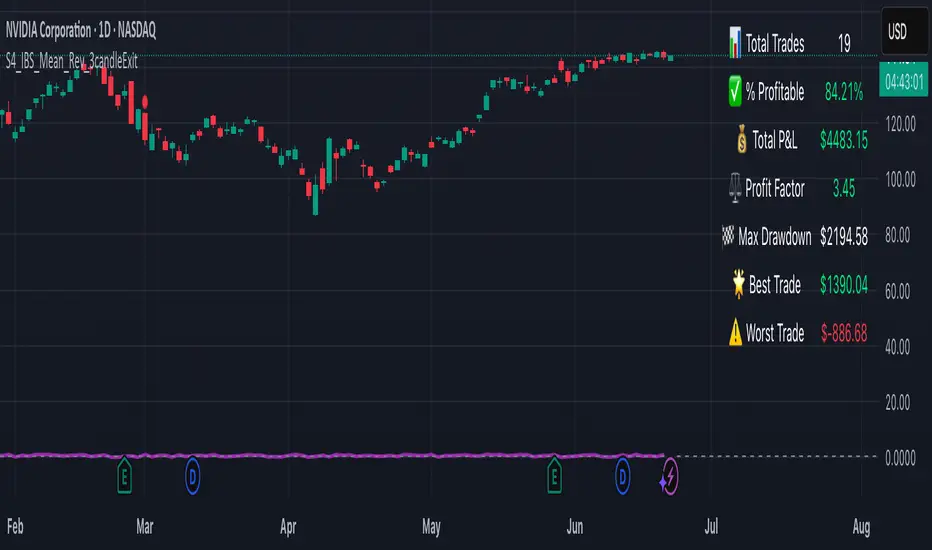
Risk and Position Sizing📏 Why Position Size Should Be Based on Risk?
Let’s say you are ready to lose 1,000 in a trade. Based on your stop loss level, you can calculate how many shares (or quantity) to buy, so that if the stop hits, you only lose that ₹1,000.
This is called risk-based position sizing. It makes your trade size dynamic — small when SL is wide, bigger when SL is tight. No more random position sizes — just systematic.
Portfolio size is multiplied by the selected risk % to get money risk per trade.
This amount is then used to calculate how many shares can be bought for the given stop-loss.
So chose your portfolio size in settings. Default Portfolio size is 1,00,000 .
You can select your risk % per portfolio in the settings — for example:
0.25% for conservative style
0.5% to 1% for balanced traders
1.25% or 1.5% for aggressive ones (not recommended for beginners)
This script will automatically calculate how much quantity you should buy, for each stop-loss scenario.
📈 Progressive & Inverse-Progressive Risk Styles
Some traders follow progressive position sizing — they start with small risk when the trend is just starting, and increase the risk % as the trend confirms.
Others follow inverse-progressive sizing — they take high risk at early stages of a bull market, and reduce risk as the trend matures (when upside becomes limited).
📌 This script allows you to manually control the risk % in settings, so you can adjust it based on your trading phase and style.
📋 Three SL Scenarios – Choose What Matches Your Style
The table shows three different stop-loss conditions, and for each one it calculates:
Today’s Low – tightest stop loss
Yesterday’s Low – slightly safer, ideal for short-term swing trades
EMA Stop (configurable) – gives more breathing room.
You can visually compare all 3 in the table and choose whichever fits your strategy and comfort.
Also, you can customize:
Theme: dark or light
Font size
Table position (upper/lower corners)
🧠 Designed for traders who take risk management seriously.
Let this script handle the math. You focus on execution.
Happy Trading!
– LensOfChartist
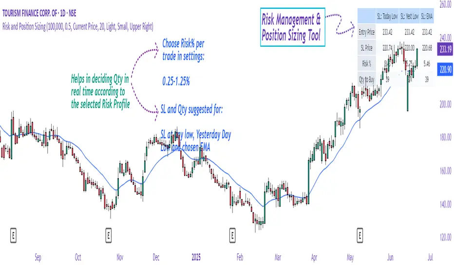
Share SizePurpose: The "Share Size" indicator is a powerful risk management tool designed to help traders quickly determine appropriate share/contract sizes based on their predefined risk per trade and the current market's volatility (measured by ATR). It calculates potential dollar differences from recent highs/lows and translates them into a recommended share/contract size, accounting for a user-defined ATR-based offset. This helps you maintain consistent risk exposure across different instruments and market conditions.
How It Works: At its core, the indicator aims to answer the question: "How many shares/contracts can I trade to keep my dollar risk within limits if my stop loss is placed at a recent high or low, plus an ATR-based buffer?"
Price Difference Calculation: It first calculates the dollar difference between the current close price and the high and low of the current bar (Now) and the previous 5 bars (1 to 5).
Tick Size & Value Conversion: These price differences are then converted into dollar values using the instrument's specific tickSize and tickValue. You can select common futures contracts (MNQ, MES, MGC, MCL), a generic "Stock" setting, or define custom values.
ATR Offset: An Average True Range (ATR) based offset is added to these dollar differences. This offset acts as a buffer, simulating a stop loss placed beyond the immediate high/low, accounting for market noise or volatility.
Risk-Based Share Size: Finally, using your Default Risk ($) input, the indicator calculates how many shares/contracts you can take for each of the 6 high/low scenarios (current bar, 5 previous bars) to ensure your dollar risk per trade remains constant.
Dynamic Table: All these calculations are presented in a clear, real-time table at the bottom-left of your chart. The table dynamically adjusts its "Label" to show the selected symbol preset, making it easy to see which instrument's settings are currently being used. The "Shares" rows indicate the maximum shares/contracts you can trade for a given risk and stop placement. The cells corresponding to the largest dollar difference (and thus smallest share size) for both high and low scenarios are highlighted, drawing your attention to the most conservative entry points.
Key Benefits:
Consistent Risk: Helps maintain a consistent dollar risk per trade, regardless of the instrument or its current price/volatility.
Dynamic Sizing: Automatically adjusts share/contract size based on market volatility and your chosen stop placement.
Quick Reference: Provides a real-time, easy-to-read table directly on your chart, eliminating manual calculations.
Informed Decision Making: Assists in quickly assessing trade opportunities and potential position sizes.
Setup Parameters (Inputs)
When you add the "Share Size" indicator to your chart, you'll see a settings dialog with the following parameters:
1. Symbol Preset:
Purpose: This is the primary setting to define the tick size and value for your chosen trading instrument.
Options:
MNQ (Micro Nasdaq 100 Futures)
MES (Micro E-mini S&P 500 Futures)
MGC (Micro Gold Futures)
MCL (Micro Crude Oil Futures)
Stock (Generic stock setting, with tick size/value of 0.01)
Custom (Allows you to manually input tick size and value)
Default: MNQ
Importance: Crucial for accurate dollar calculations. Ensure this matches the instrument you are trading.
2. Tick Size (Manual Override):
Purpose: Only used if Symbol Preset is set to Custom. This defines the smallest price increment for your instrument.
Type: Float
Default: 0.25
Hidden: This input is hidden (display=display.none) unless "Custom" is selected. You might need to change display=display.none to display=display.inline in the code if you want to see and adjust it directly in the settings for "Custom" mode.
3. Tick Value (Manual Override):
Purpose: Only used if Symbol Preset is set to Custom. This defines the dollar value of one tickSize increment.
Type: Float
Default: 0.50
Hidden: This input is hidden (display=display.none) unless "Custom" is selected. Similar to Tick Size, you might need to adjust its display property if you want it visible.
4. Default Risk ($):
Purpose: This is your maximum desired dollar risk per trade. All share size calculations will be based on this value.
Type: Float
Default: 50.0
Hidden: This input is hidden (display=display.none). It's a critical setting, so consider making it visible by changing display=display.none to display=display.inline in the code if you want users to easily adjust their risk.
ATR Offset Settings (Group): This group of settings allows you to fine-tune the ATR-based buffer added to your potential stop loss.
5. ATR Offset Length:
Purpose: Defines the lookback period for the Average True Range (ATR) calculation used for the offset.
Type: Integer
Default: 7
Hidden: This input is hidden (display=display.none).
6. ATR Offset Timeframe:
Purpose: Specifies the timeframe on which the ATR for the offset will be calculated. This allows you to use ATR from a higher timeframe for your stop buffer, even if your chart is on a lower timeframe.
Type: Timeframe string (e.g., "1" for 1 minute, "60" for 1 hour, "D" for Daily)
Default: "1" (1 Minute)
Hidden: This input is hidden (display=display.none).
7. ATR Offset Multiplier (x ATR):
Purpose: Multiplies the calculated ATR value to determine the final dollar offset added to your high/low price difference. A value of 1.0 means one full ATR is added. A value of 0.5 means half an ATR is added.
Type: Float
Minimum Value: 0 (no offset)
Default: 1.0
Hidden: This input is hidden (display=display.none).
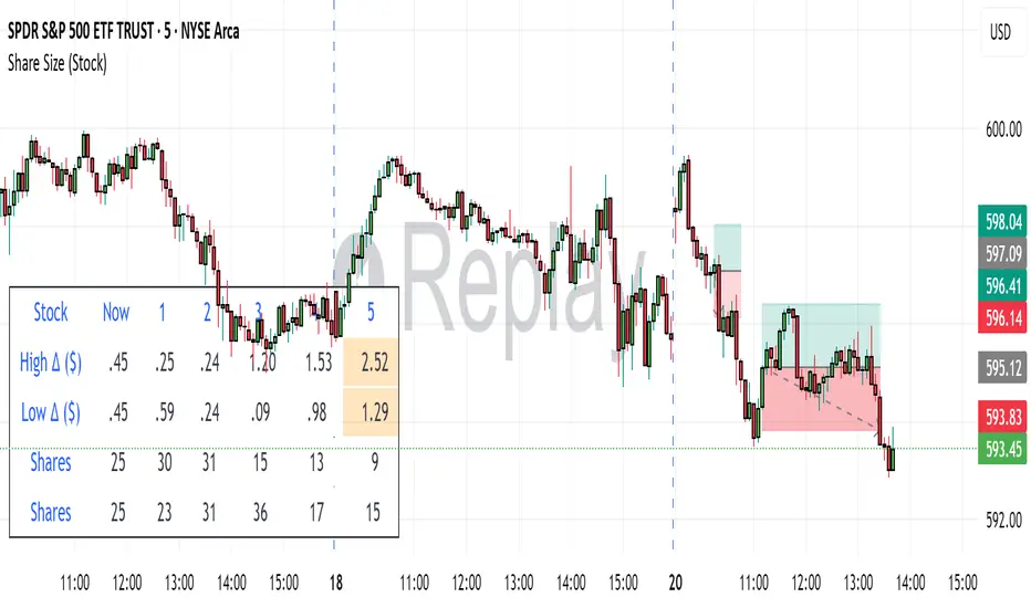
Smarter Money Flow Divergence Detector [PhenLabs]📊 Smarter Money Flow Divergence Detector
Version: PineScript™ v6
📌 Description
SMFD was developed to help give you guys a better ability to “read” what is going on behind the scenes without directly having access to that level of data. SMFD is an enhanced divergence detection indicator that identifies money flow patterns from advanced volume analysis and price action correspondence. The detection portion of this indicator combines intelligent money flow calculations with multi timeframe volume analysis to help you see hidden accumulation and distribution phases before major price movements occur.
The indicator measures institutional trading activity by looking at volume surges, price volume dynamics, and the factors of momentum to construct an overall picture of market sentiment. It’s built to assist traders in identifying high probability entries by identifying if smart money is positioning against price action.
🚀 Points of Innovation
● Advanced Smart Money Flow algorithm with volume spike detection and large trade weighting
● Multi timeframe volume analysis for enhanced institutional activity detection
● Dynamic overbought/oversold zones that adapt to current market conditions
● Enhanced divergence detection with pivot confirmation and strength validation
● Color themes with customizable visual styling options
● Real time institutional bias tracking through accumulation/distribution analysis
🔧 Core Components
● Smart Money Flow Calculation: Combines price momentum, volume expansion, and VWAP analysis
● Institutional Bias Oscillator: Tracks accumulation/distribution patterns with volume pressure analysis
● Enhanced Divergence Engine: Detects bullish/bearish divergences with multiple confirmation factors
● Dynamic Zone Detection: Automatically adjusts overbought/oversold levels based on market volatility
● Volume Pressure Analysis: Measures buying vs selling pressure over configurable periods
● Multi factor Signal System: Generates entries with trend alignment and strength validation
🔥 Key Features
● Smart Money Flow Period: Configurable calculation period for institutional activity detection
● Volume Spike Threshold: Adjustable multiplier for detecting unusual institutional volume
● Large Trade Weight: Emphasis factor for high volume periods in flow calculations
● Pivot Detection: Customizable lookback period for accurate divergence identification
● Signal Sensitivity: Three tier system (Conservative/Medium/Aggressive) for signal generation
● Themes: Four color schemes optimized for different chart backgrounds
🎨 Visualization
● Main Oscillator: Line, Area, or Histogram display styles with dynamic color coding
● Institutional Bias Line: Real time tracking of accumulation/distribution phases
● Dynamic Zones: Adaptive overbought/oversold boundaries with gradient fills
● Divergence Lines: Automatic drawing of bullish/bearish divergence connections
● Entry Signals: Clear BUY/SELL labels with signal strength indicators
● Information Panel: Real time statistics and status updates in customizable positions
📖 Usage Guidelines
Algorithm Settings
● Smart Money Flow Period
○ Default: 20
○ Range: 5-100
○ Description: Controls the calculation period for institutional flow analysis.
Higher values provide smoother signals but reduce responsiveness to recent activity
● Volume Spike Threshold
○ Default: 1.8
○ Range: 1.0-5.0
○ Description: Multiplier for detecting unusual volume activity indicating institutional participation. Higher values require more extreme volume for detection
● Large Trade Weight
○ Default: 2.5
○ Range: 1.5-5.0
○ Description: Weight applied to high volume periods in smart money calculations. Increases emphasis on institutional sized transactions
Divergence Detection
● Pivot Detection Period
○ Default: 12
○ Range: 5-50
○ Description: Bars to analyze for pivot high/low identification.
Affects divergence accuracy and signal frequency
● Minimum Divergence Strength
○ Default: 0.25
○ Range: 0.1-1.0
○ Description: Required price change percentage for valid divergence patterns.
Higher values filter out weaker signals
✅ Best Use Cases
● Trading with intraday to daily timeframes for institutional position identification
● Confirming trend reversals when divergences align with support/resistance levels
● Entry timing in trending markets when institutional bias supports the direction
● Risk management by avoiding trades against strong institutional positioning
● Multi timeframe analysis combining short term signals with longer term bias
⚠️ Limitations
● Requires sufficient volume for accurate institutional detection in low volume markets
● Divergence signals may have false positives during highly volatile news events
● Best performance on liquid markets with consistent institutional participation
● Lagging nature of volume based calculations may delay signal generation
● Effectiveness reduced during low participation holiday periods
💡 What Makes This Unique
● Multi Factor Analysis: Combines volume, price, and momentum for comprehensive institutional detection
● Adaptive Zones: Dynamic overbought/oversold levels that adjust to market conditions
● Volume Intelligence: Advanced algorithms identify institutional sized transactions
● Professional Visualization: Multiple display styles with customizable themes
● Confirmation System: Multiple validation layers reduce false signal generation
🔬 How It Works
1. Volume Analysis Phase:
● Analyzes current volume against historical averages to identify institutional activity
● Applies multi timeframe analysis for enhanced detection accuracy
● Calculates volume pressure through buying vs selling momentum
2. Smart Money Flow Calculation:
● Combines typical price with volume weighted analysis
● Applies institutional trade weighting for high volume periods
● Generates directional flow based on price momentum and volume expansion
3. Divergence Detection Process:
● Identifies pivot highs/lows in both price and indicator values
● Validates divergence strength against minimum threshold requirements
● Confirms signals through multiple technical factors before generation
💡 Note: This indicator works best when combined with proper risk management and position sizing. The institutional bias component helps identify market sentiment shifts, while divergence signals provide specific entry opportunities. For optimal results, use on liquid markets with consistent institutional participation and combine with additional technical analysis methods.

MTF Pivot Fib Speed Resistance FansOverview
This Pine Script indicator, titled "MTF Pivot Fib Speed Resistance Fans", is a multi-timeframe tool that automatically plots Fib Speed Resistance Fan lines based on pivot structures derived from higher timeframes. It mirrors the functionality of TradingView’s built-in “Fib Speed Resistance Fan” drawing tool, but in a dynamic, programmatic way. It uses pivot highs and lows to anchor fan projections, drawing forward-facing trend lines that align with well-known Fibonacci ratios and their extensions.
Pivot Detection Logic
The script identifies pivots by comparing the current bar’s high and low against the highest and lowest prices over a user-defined pivot period. This pivot detection occurs on a higher timeframe of your choice, giving a broader and more strategic view of price structure. The script tracks direction changes in the pivot trend and stores only the most recent few pivots to maintain clean and meaningful fan drawings.
Fan Direction Control
The user can select whether to draw fans for "Buys", "Sells", or "Both". The script only draws fan lines when a new directional move is detected based on the pivot structure and the selected bias. For example, in “Buys” mode, a rising pivot followed by another higher low will trigger upward fan projections.
Fib Speed Resistance Levels
Once two pivots are identified, the script draws multiple fan lines from the first pivot outward, at angles defined by a preset list of Fibonacci levels. These fan lines help visualize speed and strength of a price move.
The script also draws a horizontal line from the pivot for additional confluence at the base level (1.0).
Price Level Plotting
In addition to drawing fan lines, the indicator also plots their price levels on the right-hand price scale. This makes it easier for users to visually reference the projected support and resistance levels without needing to trace the lines manually across the chart.
Mapping to TradingView’s "Fib Speed Resistance Fan"
The expanded set of values used in this script is not arbitrary—they closely align with the default and extended levels available in TradingView's built-in "Fib Speed Resistance Fan" tool.
TradingView’s Fib Fan tool offers several levels by default, including traditional Fibonacci ratios like 0.382, 0.5, 0.618, and 1. However, if you right-click the tool and open its settings, you’ll find additional toggles for levels like 1.618, 2.000, 2.618, and even 4.000. These deeper levels are used to project stronger trend continuations beyond the standard retracement zones.
The inclusion of levels such as 0.25, 0.75, and 1.34 reflects configurations that are available when you manually add or customize levels in TradingView’s fan tool. While 1.34 is not a canonical Fibonacci ratio, it is often found in hybrid Gann/Fib methods and is included in some preset templates in TradingView’s drawing tool for advanced users.
By incorporating these levels directly into the Pine Script, the indicator faithfully reproduces the fan structure users would manually draw using TradingView’s graphical Fib Fan tool—but does so programmatically, dynamically, and with multi-timeframe control. This eliminates manual errors, allows for responsive updating, and adds custom visual tracking via the price scale.
These values are standardized within the context of TradingView's Fib Fan tool and not made up. This script automates what the manual drawing tool achieves, with added precision and flexibility.
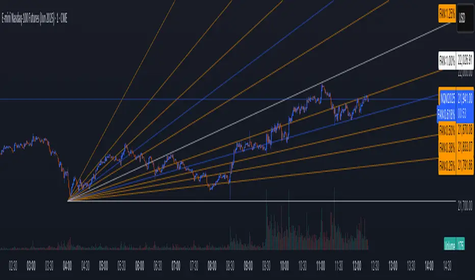
ADR by Saurabh MaggoADR levels for intraday
This Pine Script v5 indicator plots Average Daily Range (ADR) levels on a 5-minute NSE chart, ideal for intraday traders. It marks key price levels (L3+, L3-, L2+, L2-, L1+, L1-) at 9:15 AM IST each day, based on the daily open and a customizable ATR period.
Features:
Configurable Levels: Adjust ATR period (default 5) and multipliers (L3=0.5, L2=0.25, L1=0.125) to set price targets.
Today Only Option: Toggle Show Recent to display only the current day’s levels or all historical levels.
Visual Customization: Choose vibrant colors for each level via settings, with a glow effect
(toggleable, transparency=20) and adjustable circle size (default 2, range 1–5) for enhanced visibility, optimized for dark chart backgrounds.
Clean Design: Single-point plotting at 9:15 AM IST ensures a clutter-free chart, with dynamic points that move with the chart.
Usage: Perfect for NSE intraday trading, this indicator helps identify high-probability price targets. Customize levels, colors, and visuals to suit your strategy.
