Cyatophilum Swing Trader [ALERTSETUP]This is an indicator for swing trading which allows you to build your own strategies, backtest and alert. This version is the alertsetup which allows to create automated alerts hosted on TradingView servers that will trigger in form of emails, SMS, webhooks, notifications, and more. The backtest version can be found in my profile scripts page.
The particularity of this indicator is that it contains several indicators, including a custom one, that you can choose in a drop down list, as well as a trailing stop loss and take profit system.
The current indicators are :
CYATO AI: a custom indicator inspired by Donchian Channels that will catch each big trend and important reversal points .
The indicator has two major "bands" or channels and two minor bands. The major bands are bigger and are always displayed.
When price reaches a major band, acting as a support/resistance, it will either bounce on it or break through it. This is how "tops" and "bottoms", and breakouts are caught.
The minor bands are used to catch smaller moves inside the major bands. A combination of volume, momentum and price action is used to calculate the signals.
Advantages of this indicator: it should catch top and bottoms better than other swing trade indicators.
Cons of this indicator: Some minor moves might be ignored. Sometimes the script will catch a fakeout due to the Bands design.
Best timeframes to use it : 2H~4H
Sample:
Other indicators available:
SARMA: A combination of Parabolic Stop and Reverse and Exponential Moving Average (20 and 40) .
SAR: Regular Parabolic Stop and Reverse .
QQE: An indicator based on Quantitative Qualitative Estimation .
SUPERTREND: A reversal indicator based on Average True Range .
CHANNELS: The classic Donchian Channels .
More indicators might be added in the future.
About the signals: each entry (long & short) is calculated at bar close to avoid repainting. Exits (SL & TP) can either be intra-bar or at bar close using the Exit alert type parameter.
STOP LOSS SYSTEM
The base indicators listed above can be used with or without TP/SL.
TP and SL can be both turned on and off and configured for both directions.
The system can be configured with 3 parameters as follows:
Stop Loss Base % Price: Starting Value for LONG/SHORT stop loss
Trailing Stop % Price to Trigger First parameter related to the trailing stop loss. Percentage of price movement in the right direction required to make the stop loss line move.
Trailing Stop % Price Movement: Second parameter related to the trailing stop loss. Percentage for the stop loss trailing movement.
Another option is the "Reverse order on Stop Loss". Use this if you want the strategy to trigger a reverse order when a stop loss is hit.
TAKE PROFIT SYSTEM
The system can be configured with 2 parameters as follows:
Take Profit %: Take profit value in percentage of price.
Trailing Profit Deviation %: Percent deviation for the trailing take profit.
Combining indicators and Take Profit/Stop Loss
One thing to note is that if a reversal signal triggers during a trade, the trade will be closed before SL or TP is reached.
Indeed, the base indicators are reversal indicators, they will trigger long/short signals to follow the trend.
It is possible to use a takeprofit without stop loss, like in this example, knowing that the signal will reverse if the trade goes badly.
The base indicators settings can be changed in the "Advanced Parameters" section.
Configuration used for this snapshot:
ALERTS DEFINITION
Each alert correspond to the labels on chart.
01. LONG ENTRY (BUY) : Long alert
02. LONG STOP LOSS : Long stop loss event
03. LONG TAKE PROFIT : Long take profit event
04. SHORT ENTRY (SELL) : Short alert
05. SHORT STOP LOSS : Short stop loss event
06. SHORT TAKE PROFIT : Short take profit event
07. LONG EXIT : Long exit alert. Triggers on both Stop loss and Take Profit
08. SHORT EXIT : Short exit alert. Triggers on both Stop loss and Take Profit
09. ALL TAKE PROFITS : Long and Short Take Profits. Both directions.
10. ALL STOP LOSSES : Long and Short Stop Losses. Both directions.
11. ALL EXITS : Long and Short exits alert. Stop Loss and Take Profit both Long and Short.
Use the link below to obtain access to this indicator.
In den Scripts nach "stop loss" suchen

NAS Oracle AlgoThe NAS Oracle Algo is a powerful and versatile daily trading indicator designed to provide clear, automated support and resistance levels for both long and short trading strategies. By calculating a dynamic range based on the previous day's price action, it projects key entry points, stop-losses, and up to six profit targets onto your chart, giving you a complete roadmap for the trading day.
Key Features:
Dual-Sided Strategy: Generates independent levels for BUY and SELL setups, making it effective for both directional and range-bound markets.
Customizable Reference Point: Choose between using the current day's "Open" or the previous day's "Pre Close" as the base for all calculations.
Comprehensive Levels:
Entry Level: The price level to execute a trade.
Stop Loss: A predefined level to limit potential losses.
Profit Targets (1-6): Six incremental take-profit levels, allowing for partial profit-taking strategies.
Multiple Display Options:
Visual Levels & Labels: Clean horizontal lines and text labels are drawn directly on the chart for easy price reference.
Information Table: A highly customizable data table that summarizes all key levels, which can be positioned at the Top or Bottom of the chart and resized.
Flexible Configuration: Toggle the visibility of levels and choose to show either 3 or 6 profit targets to suit your trading style and avoid chart clutter.
How to Use:
Add the Indicator: Apply the "NAS Oracle Algo" to your chart. It works best on daily and intraday timeframes.
Configure Settings: In the indicator's settings, choose your preferred Option (Open/Pre Close), toggle levels and the table on/off, and adjust their position and size.
Interpret the Signals:
BUY Setup: When the price moves above the green "Buy Above" level, consider a long entry.
Stop Loss: Place your stop loss at the BUY_SL level.
Take Profit: Scale out of your position at the six progressively higher target levels (T1 to T6).
SELL Setup: When the price moves below the red "Sell Below" level, consider a short entry.
Stop Loss: Place your stop loss at the SELL_SL level.

Manipulation Model [FB]GENERAL OVERVIEW:
The Manipulation Model indicator is a complete rule-based system that identifies and confirms setups from the Funded Brothers Manipulation Model. It detects large impulsive candles, called Manipulation Candles and Almost Manipulation Candles, that form around key market levels such as session highs/lows, daily, weekly, and monthly levels, or higher timeframe Fair Value Gaps (FVGs). Using this structure, the indicator automatically marks long, short, bulltrap, and beartrap setups with predefined entry, stop loss, and take profit areas.
This indicator was developed by Flux Charts in collaboration with the Funded Brothers.
ATTRIBUTION NOTICE:
This indicator incorporates concepts and source code from the indicator “MCs with Alerts” authored by @hamza_xau on TradingView. We have received full written permission from the original author to use and commercialize this code within this invite-only script.
Original script: MCs with Alerts:
What is the purpose of the indicator?:
The indicator automates detection of the Manipulation Model trading strategy setups by combining candle structure, key levels, session timing, and higher timeframe Fair Value Gaps. It removes discretion by enforcing fixed conditions for valid signals and automatically managing entry, stop-loss, and take-profit logic.
What is the theory behind the indicator?:
The indicator is built on how price interacts with major reference points such as session highs and lows, or daily and weekly levels. These levels are commonly referenced in technical analysis as areas where price previously reversed or consolidated. Manipulation Candles identify moments when price breaks past these reference points on both sides of the prior candle before closing firmly in one direction. When these candles form near higher timeframe Fair Value Gaps, it reflects price reacting inside an area that previously showed directional imbalance. The higher timeframe EMA filter aligns all detected setups with the broader market trend, allowing only signals that match the dominant direction.
MANIPULATION MODEL FEATURES:
Manipulation Candlesticks
Almost Manipulation Candlesticks
Higher Timeframe Fair Value Gaps
Sessions
Key Levels
Signals
Dashboard
Alerts
MANIPULATION CANDLESTICKS:
Manipulation Candlesticks (MCs) are candles that sweep both sides of the previous candle’s range and close outside of it. In the Manipulation Model indicator, these candles form the foundation for the long/short setups. Once one forms, the indicator checks its position relative to sessions, key levels, and higher timeframe Fair Value Gaps to determine if a valid setup exists.
🔹What is a Manipulation Candlestick?
A Manipulation Candlestick (MC) is defined by structure rather than size. It forms when price takes out both the high and low of the previous candle, then closes outside that range.
A bullish Manipulation Candle occurs when price sweeps below the previous candle’s low and then closes above the previous candle’s high.
A bearish Manipulation Candle occurs when price sweeps above the previous candle’s high and then closes below the previous candle’s low.
🔹How to interpret and use Manipulation Candlesticks:
Manipulation Candlesticks show where price made a strong one-sided move after taking both sides of the previous candle’s range. When one forms, it marks an area where buyers or sellers were likely trapped as price moved aggressively in one direction.
A bullish MC shows strong buying after a false move lower. Price sweeps below the prior low, takes out the prior high, and closes above the previous range, confirming buyers are in control.
A bearish MC shows strong selling after a false move higher than the previous candle’s high. Price sweeps above the prior high, drops below the prior low, and closes beneath the previous range, confirming sellers are dominant.
🔹How Manipulation Candlesticks are identified:
The indicator confirms Manipulation Candles using three filters once a candle closes:
Sweep Condition:
Price must take both sides of the previous candle’s range, moving above its high and below its low, before closing outside that range.
Directional Close:
A bullish MC must close above the previous high, and a bearish MC must close below the previous low.
Wick Confirmation:
A bullish MC must have a smaller upper wick (high - close) than lower wick (open - low), and a bearish MC must have a smaller lower wick (close - low) than upper wick (high - open).
Once these conditions are met at candle close, it is confirmed as a bullish or bearish Manipulation Candle.
🔹Bullish Manipulation Candle
A bullish Manipulation Candle forms when price sweeps below the previous candle’s low, then breaks above its high, and closes above it. The lower wick must be larger than the upper wick, showing little pullback as price pushed upward and confirming strong buying pressure.
🔹Bearish Manipulation Candle
A bearish Manipulation Candle forms when price sweeps above the previous candle’s high, then drops below its low, and closes beneath it. The upper wick must be larger than the lower wick, showing little pullback as price moved downward and confirming strong selling pressure.
🔹Manipulation Candle Visuals
When the indicator detects a Manipulation Candle, it automatically changes the candle’s color on the chart. Both bullish and bearish Manipulation Candles use the same color. Users can change this color in the settings by adjusting the “Manipulation Candlestick” option found under the “Style Customization” section.
The candle coloring feature can also be turned off entirely, which only removes the visual highlight from the chart and does not affect the signals or any of the indicator’s underlying logic that uses Manipulation Candlesticks.
ALMOST MANIPULATION CANDLESTICKS:
Almost Manipulation Candlesticks (AMCs) are similar to Manipulation Candles, except they close inside the previous candle’s range instead of outside it. In the Manipulation Model indicator, these candles help identify when price is showing the same sweeping behavior but hasn’t yet confirmed full displacement. They act as early warnings that a manipulation event may be developing. Just like Manipulation Candles, the indicator checks an AMC’s position relative to sessions, key levels, and higher timeframe Fair Value Gaps to determine if a valid setup exists.
🔹What is an Almost Manipulation Candlestick?
An Almost Manipulation Candlestick (AMC) forms when price sweeps both the high and low of the previous candle and closes inside that candle’s range.
A bullish AMC occurs when price sweeps below the previous low, moves above the previous high, and closes within the previous candle’s body instead of above it.
A bearish AMC occurs when price sweeps above the previous high, drops below the previous low, and closes within the previous candle’s body instead of beneath it.
🔹How to Interpret and Use Almost Manipulation Candlesticks:
Almost Manipulation Candles highlight hesitation or early signs of manipulation.
A bullish AMC indicates buyers pushed price up after sweeping lower, but price did not close decisively above the prior high.
A bearish AMC indicates sellers pushed price down after sweeping higher, but price did not close decisively below the prior low.
🔹How Almost Manipulation Candlesticks are identified:
The indicator confirms Almost Manipulation Candles using the same sweep and wick logic as Manipulation Candles, except the candle’s close must remain inside the previous candle’s range:
Sweep Condition:
Price must take both sides of the previous candle’s range, moving above its high and below its low.
Candle Close Location:
The candle’s close must stay within the prior candle’s range.
Wick Confirmation:
For a bullish AMC, the lower wick must be larger than the upper wick. For a bearish AMC, the upper wick must be larger than the lower wick.
Once these conditions are met at candle close, it is confirmed as a bullish or bearish Almost Manipulation Candle.
🔹Bullish Almost Manipulation Candle
A bullish AMC forms when price sweeps below the previous candle’s low, moves above the prior candle’s high, and closes back inside the previous candle’s range. The lower wick must be larger than the upper wick, showing that buyers defended lower prices but the move did not close decisively upward.
🔹Bearish Almost Manipulation Candle
A bearish AMC forms when price sweeps above the previous candle’s high, drops below the previous candle’s low, and closes back inside the previous candle’s range. The upper wick must be larger than the lower wick, showing that sellers rejected higher prices but the candle did not close decisively lower.
🔹Almost Manipulation Candle Visuals
When the indicator detects an Almost Manipulation Candle, it automatically changes the candle’s color on the chart. Both bullish and bearish Almost Manipulation Candles use the same color. Users can change this color in the settings by adjusting the “Almost Manipulation Candlestick” option found under the “Style Customization” section.
The candle coloring feature can also be turned off entirely, which only removes the visual highlight from the chart and does not affect the signals or any of the indicator’s underlying logic that uses Almost Manipulation Candlesticks.
HIGHER TIMEFRAME FAIR VALUE GAPS:
The Manipulation Model indicator automatically plots Fair Value Gaps from two user-selected higher timeframes.
🔹What is a Fair Value Gap?:
A Fair Value Gap (FVG) is an area where the market’s perception of fair value suddenly changes. On your chart, it appears as a three-candle pattern: a large candle in the middle, with smaller candles on each side that don’t fully overlap it. A bullish FVG forms when a bullish candle is between two smaller bullish/bearish candles, where the first and third candles’ wicks don’t overlap each other at all. A bearish FVG forms when a bearish candle is between two smaller bullish/bearish candles, where the first and third candles’ wicks don’t overlap each other at all.
Bullish & Bearish FVGs:
🔹Why are Fair Value Gaps important?:
Fair Value Gaps (FVGs) show where price moved so quickly that one side of the market never got a chance to trade. They represent sudden shifts in what traders believe something is worth, where “fair value” changed. When a large candle drives straight through an area without overlap from the candles before and after it, it means buyers or sellers were so aggressive that the market skipped that price zone entirely.
These gaps matter because they mark the moment when confidence in price changes. If price rallies and never pulls back, it signals that traders accept the new higher prices as fair and are willing to keep buying there. The same logic applies in reverse for bearish gaps. They tell you where the market re-priced aggressively and where value was last accepted.
🔹How are Fair Value Gaps used?:
Higher Timeframe FVGs are used as a confluence for all setups within the Manipulation Model indicator. The indicator automatically detects and plots these imbalances from the chosen higher timeframe onto the current chart. When a Manipulation or Almost Manipulation Candle forms near or inside a higher timeframe Fair Value Gap, it adds context to the setup. They are not trade signals by themselves but act as a supporting element that contextualizes setups.
🔹When are Higher Timeframe Fair Value Gaps mitigated?
A Higher Timeframe Fair Value Gap is considered mitigated when the selected higher timeframe closes above the gap for a bearish FVG or below the gap for a bullish FVG.
🔹Higher Timeframe FVG Settings:
Timeframe 1 / Timeframe 2:
Select up to two higher timeframes to use for Fair Value Gaps. Disabling either one removes it visually from the chart but does not affect signal generation. However, the timeframes you select will be used for signal generation logic.
For example, if you select the 1-hour and 4-hour timeframes, then the 1-hour and 4-hour FVGs will be used for signal generation logic, which is explained in the signals section below.
Combine Zones:
When enabled, overlapping FVGs on the same higher timeframe are merged into a single zone. This keeps the chart clean and prevents duplicate zones from displaying.
Midline:
Adds a center line through each higher timeframe FVG.
Labels:
Displays a “ FVG” label beside each zone. This helps users see which timeframe the FVG is detected from.
Color Customization:
Each timeframe has separate color settings for bullish and bearish FVGs. Users can adjust these colors independently for both timeframes to fit their chart layout.
FVG Display Limit:
Controls how many higher timeframe FVGs are shown at once. Only the nearest X active gaps to current price will appear, helping maintain a clear view of relevant imbalances.
SESSIONS:
The Manipulation Model indicator includes six customizable trading sessions: Asia, London, NY AM, NYSE, London Close, and NY PM. All session times and visuals are fully user-configurable. Each session has adjustable start and end times that can be set to match your preferred schedule. Users can also customize visuals for each session, including the color, opacity, and visibility of session zones.
Session highs and lows are automatically tracked and used within the indicator’s signal logic. When a Manipulation or Almost Manipulation Candle forms near a session high or low, it is recognized within the indicator’s signal detection.
Default times used for each session (in EST):
Asia: 20:00 - 00:00
London: 02:00 - 05:00
NY AM: 08:00 - 09:30
NYSE: 09:30 - 10:00
London Close: 10:00 - 11:00
NY PM: 11:00 - 14:00
🔹Session Settings:
Session Boxes:
Each session has a box that outlines its active time window. These boxes can be toggled on or off independently. When active, they visually separate each part of the trading day. Users can adjust the color and opacity of each session box.
Session Highs/Lows:
Every session can display its own high and low as horizontal lines. Users can customize the line style for session highs/lows, choosing between solid, dashed, or dotted. The color of the lines will match the same color used for the session box.
Labels and Price Display:
Labels can be toggled on for all session highs and lows. Users can adjust label color, text size, and choose whether to show the price next to the label. Users can adjust the text size, choosing between tiny, small, normal, large, and huge.
Extend Levels:
When enabled, each session’s high and low levels can be extended forward by a set number of bars.
Session Titles:
Titles for each enabled session (e.g., “Asia,” “London,” “NY AM”) can be displayed directly on the chart.
Show Last:
The “Show Last” setting allows you to choose how many recent sessions of each type appear on the chart. For example, if you only have the Asia session enabled and have this setting set to 2, the recent two Asia sessions will be displayed.
🔹Sessions Used
Under the “Sessions Used” section in the settings, users can choose which sessions are active for signal generation. Only sessions enabled here will produce signals. For example, if you want setups to form only during the London session, turn off all other sessions in this section.
Disabling a session under the main Sessions section only hides its visuals (boxes, lines, or labels). It does not impact signal detection or logic. However, changing a session’s start and end time in either section will affect signals, since signals are tied to the exact session windows defined by the user. This distinction ensures you have full control over what’s displayed visually versus what contributes to active trade signal logic.
Please Note: Signals are only detected and plotted on your chart during sessions. Signals can not be detected outside of session time windows.
KEY LEVELS:
The Manipulation Model indicator includes 10 key market levels that outline important structural price areas across daily, weekly, and monthly timeframes. These levels include the Daily Open, Previous Day High/Low, Weekly Open, Previous Week High/Low, Monthly Open, Previous Month High/Low, and Midnight Open. The levels can be enabled or disabled and customized in color and line style. These levels are used for the indicator’s signal logic.
🔹Daily Open
The Daily Open marks where the current trading day began.
🔹Previous Day High/Low
The Previous Day High (PDH) marks the highest price reached during the previous regular trading session. It shows where buyers pushed price to its highest point before the market closed. This value is automatically pulled from the daily chart and projected forward onto intraday timeframes.
The Previous Day Low (PDL) marks the lowest price reached during the previous regular trading session. It shows where selling pressure reached its lowest point before buyers stepped in. Like the PDH, this level is retrieved from the prior day’s data and extended into the current session.
🔹Weekly Open
The Weekly Open marks the first price of the current trading week.
🔹Previous Week High/Low
The Previous Week High (PWH) marks the highest price reached during the previous trading week. It shows where buying pressure reached its peak before the weekly close. This value is automatically pulled from the weekly chart and extended forward into the current week for easy reference on intraday timeframes.
The Previous Week Low (PWL) marks the lowest price reached during the previous trading week. It shows where sellers pushed price to its lowest point before buyers regained control. Like the PWH, this level is sourced from the prior week’s data and projected onto the current week’s chart.
🔹Monthly Open
The Monthly Open marks the opening price of the current month.
🔹Previous Month High/Low
The Previous Month High (PMH) marks the highest price reached during the previous calendar month. It represents the point at which buyers achieved the strongest push before the monthly close. This level is automatically retrieved from the monthly chart and extended into the new month on all lower timeframes.
The Previous Month Low (PML) marks the lowest price reached during the previous calendar month. It shows where selling pressure was strongest before buyers stepped back in. Like the PMH, this value is pulled from the prior month’s data and extended into the new month on all lower timeframes.
🔹Midnight Open
The Midnight Open marks the first price of the trading day at 00:00 EST.
🔹Customization Options:
Users can fully customize the appearance of all key levels, including the following:
Daily Levels: Daily Open, PDH, and PDL
Weekly Levels: Weekly Open, PWH, and PWL
Monthly Levels: Monthly Open, PMH, and PML
Midnight Open
Color Settings:
Each group of levels (Daily, Weekly, Monthly) shares a single color for the Open, High, and Low lines. For example, the Daily Open, PDH, and PDL all use the same color. Colors can be changed for each group, but not for individual levels within the same group.
Line Style:
Users can select a global line style, choosing between solid, dashed, or dotted, for all Daily, Weekly, and Monthly levels. This style applies to all levels within those groups. For example, the Weekly Open, PWH, and PWL must all share the same line style.
The Midnight Open has its own independent line style setting and can use a different style from the other key levels.
Show Labels:
When enabled, text labels appear to the right of each key level. Users can adjust label color, but only one label color is applied to all levels for consistency.
🔹Key Levels Used:
Under the “Key Levels Used” section, users can choose which Key Levels and Session Levels (Session Highs/Lows) are factored into signal generation. Only levels enabled here are considered within the logic that confirms setups.
Users can choose between the following levels:
Daily Open
Previous Day High/Low
Weekly Open
Previous Week High/Low
Monthly Open
Previous Month High/Low
Asia Session High/Low
London Session High/Low
NY AM Session High/Low
NY Lunch Session High/Low
NY PM Session High/Low
London Close Session High/Low
Midnight Open
For example, if you only want to see setups that form using the Daily and Weekly levels, you should only enable the Daily Open, Previous Day High/Low, Weekly Open, and Previous Week High/Low.
Disabling a level in the main “Key Levels” section only hides its visuals, while disabling it in “Key Levels Used” removes it entirely from the signal logic. Adjusting or removing any level in this section directly affects how setups are detected since the indicator references these levels when confirming Long, Short, Bulltrap, and Beartrap setups.
SIGNALS:
The Manipulation Model indicator automatically identifies Long, Short, Bulltrap, and Beartrap setups based on the interaction between Manipulation Candles (MCs), Almost Manipulation Candles (AMCs), and two main entry conditions: Key Levels and Fair Value Gaps (FVGs).
Each signal type uses the structure of a Manipulation or Almost Manipulation Candle as its foundation. When one of these candles forms and aligns with the entry conditions, the indicator automatically plots labels for an entry, stop loss (SL), and take profit (TP). Every signal follows a mechanical set of rules and is marked in real time. Once confirmed on a candle close, the signal remains fixed on the chart and does not repaint.
🔹Higher Timeframe Bias Filter
Before a signal is generated, the indicator automatically determines directional bias using the 50-period Exponential Moving Average (EMA) on the 1-hour timeframe.
If price is above the 50 EMA, only bullish setups are allowed.
If price is below the 50 EMA, only bearish setups are allowed.
🔹Stop Loss and Take Profit Logic:
For every setup, the stop loss is placed at the low of the Manipulation or Almost Manipulation Candle for bullish setups, and at the high for bearish setups. The take profit is automatically calculated at a 1:1 risk-to-reward ratio relative to that distance.
Users can adjust both the SL Multiplier and TP Multiplier in the settings, under the “General Configuration” section, to extend or contract these levels. For example, increasing the TP Multiplier to 1.5 sets the take profit at 1.5x the distance between the entry and stop loss.
🔹Signal Input Settings:
Candle Type:
Choose which candle type is used to generate signals. Options include:
Manipulation Candle (MC) only
Almost Manipulation Candle (AMC) only
Both (signals are generated from either candle type)
Entry Method:
Determines whether signals are generated based on:
Key Levels only
Fair Value Gaps only
Both (signals are generated from Key Levels AND Fair Value Gaps)
Setup Types:
You can enable or disable specific setup types. Only the selected setup types will appear on your chart:
Long Setups
Short Setups
Bulltrap Setups
Beartrap Setups
🔹Long Setup – Manipulation Candle + Key Level:
A long setup forms when a bullish Manipulation Candle touches a toggled-on key level under the “Key Levels Used” section and closes above it during a toggled-on session from the “Sessions Used” section. After the candle closes and price is above the 1-hour 50 EMA, the indicator marks:
Entry: At the close of the bullish Manipulation Candle
Stop Loss: At the low of the same candle
Take Profit: Equal distance above the entry, based on TP multiplier
In this example, a bullish MC touches the PDH during the London Session and closes above the level:
🔹Short Setup – Manipulation Candle + Key Level
A short setup forms when a bearish Manipulation Candle touches a toggled-on key level under the “Key Levels Used” section and closes below it during a toggled-on session from the “Sessions Used” section. After the candle closes and price is below the 1-hour 50 EMA, the indicator marks:
Entry: At the close of the bearish Manipulation Candle
Stop Loss: At the high of the same candle
Take Profit: Equal distance below the entry, based on the TP Multiplier
In this example, a bearish MC touches the Daily Open during the NY AM Session and closes below the level:
🔹Trap Confirmation Settings
Two settings control how bulltrap and beartrap setups are confirmed once a Manipulation or Almost Manipulation Candle forms.
Candles Between Confirmation:
This setting defines the maximum number of candles allowed between the initial Manipulation Candle and the confirmation candle that closes back in the opposite direction.
For example, if this value is set to 2, the confirmation candle must appear within two bars of the Manipulation Candle for the setup to remain valid. If too many candles form in between, the bull/bear trap setup is ignored.
Trap Wick-to-Body Ratio:
This input measures the ratio of the confirmation candle’s wick size to its body size for bulltrap and beartrap setups. Lower values require a larger body compared to the wick, meaning the confirmation candle must close more decisively. If the ratio is above the threshold set by the user, the confirmation candle for a bulltrap/beartrap setup is considered valid.
For example, if the wick is 10 points and the body is 10 points, the ratio is 1.0 (10 / 10). If the wick is 10 points and the body is 20 points, the ratio is 0.5 (10 / 20).
🔹Beartrap Setup – Manipulation Candle + Key Level
A beartrap setup forms when a bearish Manipulation Candle touches a toggled-on key level under the “Key Levels Used” section. The candle does not need to close above or below the level, it only needs to touch it. After this bearish MC forms, a confirmation candle must close back above the MC’s high during an enabled session under the “Sessions Used” section. The sweep or initial touch can occur before or outside the session, but the confirmation candle must close within an active session window.
To confirm the setup, the following conditions must be met:
The confirmation candle must close within the limit set by the Candles Between Confirmation input.
Its wick-to-body ratio must be less than or equal to the Trap Wick-to-Body Ratio input
Once these conditions are met and price is above the 1-hour 50 EMA, the indicator marks:
Entry: At the close of the confirmation candle
Stop Loss: At the low of the confirmation candle
Take Profit: Equal distance above the entry, measured 1:1 from the candle’s body and scaled by the TP Multiplier
In this example, a bearish Manipulation Candle touches the Daily Open level before price reverses and a confirmation candle closes above it. The confirmation candle occurs during the Asia Session, has a strong body with minimal wicks, meeting the Trap Wick-to-Body Ratio requirement, and it forms just two candles after the bearish MC which is within the limit set by the Candles Between Confirmation input.
🔹Bulltrap Setup – Manipulation Candle + Key Level
A bulltrap setup forms when a bullish Manipulation Candle touches a toggled-on key level under the “Key Levels Used” section. The MC does not need to close above or below the level, it only needs to touch it. After this bullish MC forms, a confirmation candle must close back below the MC’s low during an enabled session under the “Sessions Used” section. The initial key level touch from the MC can occur before or outside the session, but the confirmation candle must close within an active session window.
To confirm the setup, the following conditions must be met:
The confirmation candle must close within the limit set by the Candles Between Confirmation input.
Its wick-to-body ratio must be less than or equal to the Trap Wick-to-Body Ratio input.
Once these conditions are met and price is below the 1-hour 50 EMA, the indicator marks:
Entry: At the close of the confirmation candle
Stop Loss: At the high of the confirmation candle
Take Profit: Equal distance below the entry, measured 1:1 from the candle’s body and scaled by the TP Multiplier
In this example, a bullish Manipulation Candle touches the Daily Open level before price reverses and a confirmation candle closes below it. The confirmation candle forms during the NY AM Session, has a strong body with minimal wicks that meet the Trap Wick-to-Body Ratio requirement, and it appears two candles after the bullish MC which is within the limit defined by the Candles Between Confirmation input.
🔹Long Setup – Almost Manipulation Candle + Key Level
A long setup forms when a bullish Almost Manipulation Candle (AMC) touches a toggled-on key level under the “Key Levels Used” section and closes above it during a toggled-on session from the “Sessions Used” section. After the candle closes and price is above the 1-hour 50 EMA, the indicator marks:
Entry: At the close of the bullish Almost Manipulation Candle
Stop Loss: At the low of the same candle
Take Profit: Equal distance above the entry, based on the TP Multiplier
In this example, a bullish AMC touches the Daily Open during the NYSE Session and closes above the level.
🔹Short Setup – Almost Manipulation Candle + Key Level
A short setup forms when a bearish Almost Manipulation Candle (AMC) touches a toggled-on key level under the “Key Levels Used” section and closes below it during a toggled-on session from the “Sessions Used” section. After the candle closes and price is below the 1-hour 50 EMA, the indicator marks:
Entry: At the close of the bearish Almost Manipulation Candle
Stop Loss: At the high of the same candle
Take Profit: Equal distance below the entry, based on the TP Multiplier
In this example, a bearish AMC touches the Midnight Open during the NY AM Session and closes below the level.
🔹Beartrap Setup – Almost Manipulation Candle + Key Level
A beartrap setup forms when a bearish Almost Manipulation Candle (AMC) touches a toggled-on key level under the “Key Levels Used” section. The candle does not need to close above or below the level, it only needs to touch it. After this bearish AMC forms, a confirmation candle must close back above the AMC’s high during an enabled session under the “Sessions Used” section. The initial touch can occur before or outside the session, but the confirmation candle must close within an active session window.
To confirm the setup, the following conditions must be met:
The confirmation candle must close within the limit set by the Candles Between Confirmation input.
Its wick-to-body ratio must be less than or equal to the Trap Wick-to-Body Ratio input.
Once these conditions are met and price is above the 1-hour 50 EMA, the indicator marks:
Entry: At the close of the confirmation candle
Stop Loss: At the low of the confirmation candle
Take Profit: Equal distance above the entry, measured 1:1 from the candle’s body and scaled by the TP Multiplier
In this example, a bearish AMC touches the Midnight Open before price reverses and a confirmation candle closes above it. The confirmation candle forms during the London Session, has a large body with minimal wicks that meet the Trap Wick-to-Body Ratio requirement, and appears seven candles after the bearish AMC which is within the Candles Between Confirmation limit (10 by default).
🔹Bulltrap Setup – Almost Manipulation Candle + Key Level
A bulltrap setup forms when a bullish AMC touches a toggled-on key level under the “Key Levels Used” section. The candle does not need to close above or below the level; it only needs to touch it. After this bullish AMC forms, a confirmation candle must close back below the AMC’s low during an enabled session under the “Sessions Used” section. The initial touch can occur before or outside the session, but the confirmation candle must close within an active session window.
To confirm the setup, the following conditions must be met:
The confirmation candle must close within the limit set by the Candles Between Confirmation input.
Its wick-to-body ratio must be less than or equal to the Trap Wick-to-Body Ratio input.
Once these conditions are met and price is below the 1-hour 50 EMA, the indicator marks:
Entry: At the close of the confirmation candle
Stop Loss: At the high of the confirmation candle
Take Profit: Equal distance below the entry, measured 1:1 from the candle’s body and scaled by the TP Multiplier
In this example, a bullish AMC touches the NY Lunch Session Low before price reverses and a confirmation candle closes below it. The confirmation candle forms during the Asia Session, has a strong body with minimal wicks that meet the Trap Wick-to-Body Ratio requirement, and appears six candles after the bullish AMC which is within the Candles Between Confirmation limit.
🔹Long Setup – Manipulation Candle + Fair Value Gap
A long setup forms when a bullish Manipulation Candle touches a bullish higher timeframe Fair Value Gap (FVG) from one of the two higher timeframe inputs under the “Fair Value Gaps” section. The candle must close during an enabled session under the “Sessions Used” section. After the candle closes and price is above the 1-hour 50 EMA, the indicator marks:
Entry: At the close of the bullish Manipulation Candle
Stop Loss: At the low of the same candle
Take Profit: Equal distance above the entry, scaled by the TP Multiplier
In this example, a bullish MC taps into a bullish 1-hour FVG during the Asia Session.
🔹Short Setup – Manipulation Candle + Fair Value Gap
A short setup forms when a bearish Manipulation Candle touches a bearish higher timeframe FVG from one of the two selected higher timeframe inputs under the “Fair Value Gaps” section. The candle must also close during an enabled session under the “Sessions Used” section. After the candle closes and price is below the 1-hour 50 EMA, the indicator marks:
Entry: At the close of the bearish Manipulation Candle
Stop Loss: At the high of the same candle
Take Profit: Equal distance below the entry, scaled by the TP Multiplier
In this example, a bearish MC taps a bearish 1-hour FVG during the Asia Session.
🔹Beartrap Setup – Manipulation Candle + Fair Value Gap
A beartrap setup forms when a bearish Manipulation Candle touches a bullish or bearish higher timeframe FVG from one of the two higher timeframe inputs under the “Higher Timeframe FVG Settings” section. After the bearish MC forms, price must reverse and a confirmation candle must close above the bearish MC’s high during an enabled session under the “Sessions Used” section. The initial touch of the FVG can occur before or outside the session, but the confirmation candle must close within an active session window.
To confirm the setup, the following conditions must be met:
The confirmation candle must close within the limit set by the Candles Between Confirmation input.
Its wick-to-body ratio must be less than or equal to the Trap Wick-to-Body Ratio input.
Once these conditions are met and price is above the 1-hour 50 EMA, the indicator marks:
Entry: At the close of the confirmation candle
Stop Loss: At the low of the confirmation candle
Take Profit: Equal distance above the entry, measured 1:1 from the candle’s body and scaled by the TP Multiplier
In this example, a bearish MC taps a 1-hour bearish FVG, price reverses, and a confirmation candle closes above the bearish MC’s high. The confirmation candle forms during the London Session, has a strong body with minimal wicks that meet the Trap Wick-to-Body Ratio requirement, and appears two candles after the bearish MC which is within the Candles Between Confirmation limit.
🔹Bulltrap Setup – Manipulation Candle + Fair Value Gap
A bulltrap setup forms when a bullish MC touches a bearish or bullish higher timeframeFVG from one of the two higher timeframe inputs under the “Higher Timeframe FVG Settings” section. After the bullish MC forms, price must reverse and a confirmation candle must close below the MC’s low during an enabled session under the “Sessions Used” section. The initial touch of the FVG can occur before or outside the session, but the confirmation candle must close within an active session window.
To confirm the setup, the following conditions must be met:
The confirmation candle must close within the limit set by the Candles Between Confirmation input.
Its wick-to-body ratio must be less than or equal to the Trap Wick-to-Body Ratio input.
Once these conditions are met and price is below the 1-hour 50 EMA, the indicator marks:
Entry: At the close of the confirmation candle
Stop Loss: At the high of the confirmation candle
Take Profit: Equal distance below the entry, measured 1:1 from the candle’s body and scaled by the TP Multiplier
In this example, a bullish MC taps a 4-hour bearish FVG, price reverses, and a confirmation candle closes below the bullish MC’s low. The confirmation candle forms during the NY PM Session, has a strong body with minimal wicks that meet the Trap Wick-to-Body Ratio requirement, and appears six candles after the bullish MC which is within the Candles Between Confirmation limit.
🔹Long Setup – Almost Manipulation Candle + Fair Value Gap
A long setup forms when a bullish AMC touches a bullish higher timeframe FVG from one of the two higher timeframe inputs under the “Fair Value Gaps” section. The candle must close during an enabled session under the “Sessions Used” section. After the candle closes and price is above the 1-hour 50 EMA, the indicator marks:
Entry: At the close of the bullish AMC
Stop Loss: At the low of the same candle
Take Profit: Equal distance above the entry, scaled by the TP Multiplier
In this example, a bullish AMC taps into a bullish 1-hour FVG during the London Session.
🔹Short Setup – Almost Manipulation Candle + Fair Value Gap
A short setup forms when a bearish AMC touches a bearish higher timeframe FVG from one of the two selected higher timeframe inputs under the “Fair Value Gaps” section. The candle must also close during an enabled session under the “Sessions Used” section. After the candle closes and price is below the 1-hour 50 EMA, the indicator marks:
Entry: At the close of the bearish AMC
Stop Loss: At the high of the same candle
Take Profit: Equal distance below the entry, scaled by the TP Multiplier
In this example, a bearish AMC taps a bearish 1-hour FVG during the NY PM Session.
🔹Beartrap Setup – Almost Manipulation Candle + Fair Value Gap
A beartrap setup forms when a bearish AMC touches a bullish or bearish higher timeframe FVG from one of the two higher timeframe inputs under the “Higher Timeframe FVG Settings” section. After the bearish AMC forms, price must reverse and a confirmation candle must close above the bearish AMC’s high during an enabled session under the “Sessions Used” section. The initial touch of the FVG can occur before or outside the session, but the confirmation candle must close within an active session window.
To confirm the setup, the following conditions must be met:
The confirmation candle must close within the limit set by the Candles Between Confirmation input.
Its wick-to-body ratio must be less than or equal to the Trap Wick-to-Body Ratio input.
Once these conditions are met and price is above the 1-hour 50 EMA, the indicator marks:
Entry: At the close of the confirmation candle
Stop Loss: At the low of the confirmation candle
Take Profit: Equal distance above the entry, measured 1:1 from the candle’s body and scaled by the TP Multiplier
In this example, a bearish AMC taps a 4-hour bearish FVG, price reverses, and a confirmation candle closes above the bearish AMC’s high. The confirmation candle forms during the NY PM Session, has a strong body with minimal wicks that meet the Trap Wick-to-Body Ratio requirement, and appears seven candles after the bearish AMC, which is within the Candles Between Confirmation limit.
🔹Bulltrap Setup – Almost Manipulation Candle + Fair Value Gap
A bulltrap setup forms when a bullish AMC touches a bearish or bullish higher timeframe FVG from one of the two higher timeframe inputs under the “Higher Timeframe FVG Settings” section. After the bullish AMC forms, price must reverse and a confirmation candle must close below the AMC’s low during an enabled session under the “Sessions Used” section. The initial touch of the FVG can occur before or outside the session, but the confirmation candle must close within an active session window.
To confirm the setup, the following conditions must be met:
The confirmation candle must close within the limit set by the Candles Between Confirmation input.
Its wick-to-body ratio must be less than or equal to the Trap Wick-to-Body Ratio input.
Once these conditions are met and price is below the 1-hour 50 EMA, the indicator marks:
Entry: At the close of the confirmation candle
Stop Loss: At the high of the confirmation candle
Take Profit: Equal distance below the entry, measured 1:1 from the candle’s body and scaled by the TP Multiplier
In this example, a bullish AMC taps a 1-hour bullish FVG, price reverses, and a confirmation candle closes below the bullish AMC’s low. The confirmation candle forms during the Asia Session, has a strong body with minimal wicks that meet the Trap Wick-to-Body Ratio requirement, and appears six candles after the bullish AMC, which is within the Candles Between Confirmation limit.
🔹Signal Style Customization
The Manipulation Model indicator provides full visual customization for all signal elements, allowing users to easily adjust the appearance of entry, stop loss, and take profit labels.
Label Colors:
Users can customize the label color for Long Setups (Long and Beartrap) and Short Setups (Short and Bulltrap).
Long and Beartrap setups share the same label color.
Short and Bulltrap setups share the same label color.
Label text color can also be customized and applied globally to all signal labels.
Stop Loss (SL) and Take Profit (TP) Labels:
The SL and TP label colors can be customized independently.
Users can toggle SL Labels and TP Labels on or off. When turned off, the corresponding labels are hidden, but their levels remain active on the chart.
Entry, Stop Loss, and Take Profit Lines:
Each of these lines can be individually toggled on or off.
Entry Line: Marks the entry price level.
Stop Loss Line: Displays the SL level derived from each setup’s logic.
Take Profit Line: Displays the TP level calculated using the Take Profit Multiplier setting.
Users can also toggle the labels for each line on or off and adjust the color for each line type independently.
WIN RATE DASHBOARD:
The Win Rate Dashboard gives traders a quick way to see the recent performance of their enabled setups. It automatically calculates and displays win rates for each signal type turned on under the “General Configuration” section, based on the sessions and key levels currently active in the settings.
The dashboard updates in real time, showing both the win rate percentage and total trade count for all enabled signal types combined. It looks back at a set number of bars to calculate results, providing a simple performance snapshot directly on your chart.
How It Works:
When a signal triggers, the indicator tracks whether price first reaches the Take Profit (TP) or Stop Loss (SL) level.
A winning trade is recorded when the take profit is hit before the stop loss.
A losing trade is recorded when the stop loss is hit before the take profit.
The win rate = (Winning Trades / Total Trades) x 100
🔹Dashboard Customization:
Users can adjust the dashboard’s appearance with the following settings:
Background Color
Frame Color
Border Color
Text Color
You can also toggle the dashboard on or off from the settings menu. It appears in the top-right corner of the chart by default and its position cannot be changed.
🔹Disclaimer:
The Win Rate Dashboard provides historical performance data based on the signals and conditions you’ve enabled. These results are calculated from past bars and are not indicative of future performance or profitability.
ALERTS:
The Manipulation Model indicator includes full alert functionality powered by AnyAlert(), allowing users to receive notifications for all major setups and level breaks in real time.
Users can choose exactly which alerts they want to receive under the “Alerts” section of the settings. Once your preferred alerts are toggled on, you can create a TradingView alert using the AnyAlert() condition. This will automatically trigger alerts for all selected events as they occur on your chart.
Available Alerts:
Long Setup
Short Setup
Bulltrap Setup
Beartrap Setup
Manipulation Candle
Almost Manipulation Candle
Previous Day High/Low Break
Current Day Open Break
Previous Week High/Low Break
Current Week Open Break
Previous Month High/Low Break
Current Month Open Break
Asia Session High/Low Break
London Session High/Low Break
NY AM Session High/Low Break
NYSE Session High/Low Break
London Close Session High/Low Break
NY PM Session High/Low Break
Midnight Open Break
To receive alerts:
Open the alert creation window in TradingView
Select “Manipulation Model ” as the condition
Choose AnyAlert() from the dropdown
Create the alert
IMPORTANT NOTES:
TradingView has limitations when running features on multiple timeframes, which can result in the following restriction:
Computation Error:
The computation of using MTF features is very intensive on TradingView. This can sometimes cause calculation timeouts. When this occurs, simply force the recalculation by modifying one indicator’s settings or by removing the indicator and adding it to your chart again.
UNIQUENESS:
The Manipulation Model is unique because every setup type is fully rule-based and tied to strict structural logic. Traders can control exactly how signals form by selecting which candle types are used, which key levels and sessions are active, and whether entries trigger from Key Levels, Fair Value Gaps, or both. All setups use objective rules for confirmation, wick-to-body ratio, and higher timeframe bias. The indicator also provides full customization for visuals, alerts, and trade parameters like TP and SL multipliers. A built-in Win Rate Dashboard tracks real-time performance for all enabled setup types based on the user’s active sessions and signal filters. Together, these features make it a complete, mechanical implementation of the Funded Brothers Manipulation Model and it works across all asset classes including stocks, crypto, forex, and futures.

Hellenic EMA Matrix - PremiumHellenic EMA Matrix - Alpha Omega Premium
Complete User Guide
Table of Contents
Introduction
Indicator Philosophy
Mathematical Constants
EMA Types
Settings
Trading Signals
Visualization
Usage Strategies
FAQ
Introduction
Hellenic EMA Matrix is a premium indicator based on mathematical constants of nature: Phi (Phi - Golden Ratio), Pi (Pi), e (Euler's number). The indicator uses these universal constants to create dynamic EMAs that adapt to the natural rhythms of the market.
Key Features:
6 EMA types based on mathematical constants
Premium visualization with Neon Glow and Gradient Clouds
Automatic Fast/Mid/Slow EMA sorting
STRONG signals for powerful trends
Pulsing Ribbon Bar for instant trend assessment
Works on all timeframes (M1 - MN)
Indicator Philosophy
Why Mathematical Constants?
Traditional EMAs use arbitrary periods (9, 21, 50, 200). Hellenic Matrix goes further, using universal mathematical constants found in nature:
Phi (1.618) - Golden Ratio: galaxy spirals, seashells, human body proportions
Pi (3.14159) - Pi: circles, waves, cycles
e (2.71828) - Natural logarithm base: exponential growth, radioactive decay
Markets are also a natural system composed of millions of participants. Using mathematical constants allows tuning into the natural rhythms of market cycles.
Mathematical Constants
Phi (Phi) - Golden Ratio
Phi = 1.618033988749895
Properties:
Phi² = Phi + 1 = 2.618
Phi³ = 4.236
Phi⁴ = 6.854
Application: Ideal for trending movements and Fibonacci corrections
Pi (Pi) - Pi Number
Pi = 3.141592653589793
Properties:
2Pi = 6.283 (full circle)
3Pi = 9.425
4Pi = 12.566
Application: Excellent for cyclical markets and wave structures
e (Euler) - Euler's Number
e = 2.718281828459045
Properties:
e² = 7.389
e³ = 20.085
e⁴ = 54.598
Application: Suitable for exponential movements and volatile markets
EMA Types
1. Phi (Phi) - Golden Ratio EMA
Description: EMA based on the golden ratio
Period Formula:
Period = Phi^n × Base Multiplier
Parameters:
Phi Power Level (1-8): Power of Phi
Phi¹ = 1.618 → ~16 period (with Base=10)
Phi² = 2.618 → ~26 period
Phi³ = 4.236 → ~42 period (recommended)
Phi⁴ = 6.854 → ~69 period
Recommendations:
Phi² or Phi³ for day trading
Phi⁴ or Phi⁵ for swing trading
Works excellently as Fast EMA
2. Pi (Pi) - Circular EMA
Description: EMA based on Pi for cyclical movements
Period Formula:
Period = Pi × Multiple × Base Multiplier
Parameters:
Pi Multiple (1-10): Pi multiplier
1Pi = 3.14 → ~31 period (with Base=10)
2Pi = 6.28 → ~63 period (recommended)
3Pi = 9.42 → ~94 period
Recommendations:
2Pi ideal as Mid or Slow EMA
Excellently identifies cycles and waves
Use on volatile markets (crypto, forex)
3. e (Euler) - Natural EMA
Description: EMA based on natural logarithm
Period Formula:
Period = e^n × Base Multiplier
Parameters:
e Power Level (1-6): Power of e
e¹ = 2.718 → ~27 period (with Base=10)
e² = 7.389 → ~74 period (recommended)
e³ = 20.085 → ~201 period
Recommendations:
e² works excellently as Slow EMA
Ideal for stocks and indices
Filters noise well on lower timeframes
4. Delta (Delta) - Adaptive EMA
Description: Adaptive EMA that changes period based on volatility
Period Formula:
Period = Base Period × (1 + (Volatility - 1) × Factor)
Parameters:
Delta Base Period (5-200): Base period (default 20)
Delta Volatility Sensitivity (0.5-5.0): Volatility sensitivity (default 2.0)
How it works:
During low volatility → period decreases → EMA reacts faster
During high volatility → period increases → EMA smooths noise
Recommendations:
Works excellently on news and sharp movements
Use as Fast EMA for quick adaptation
Sensitivity 2.0-3.0 for crypto, 1.0-2.0 for stocks
5. Sigma (Sigma) - Composite EMA
Description: Composite EMA combining multiple active EMAs
Composition Methods:
Weighted Average (default):
Sigma = (Phi + Pi + e + Delta) / 4
Simple average of all active EMAs
Geometric Mean:
Sigma = fourth_root(Phi × Pi × e × Delta)
Geometric mean (more conservative)
Harmonic Mean:
Sigma = 4 / (1/Phi + 1/Pi + 1/e + 1/Delta)
Harmonic mean (more weight to smaller values)
Recommendations:
Enable for additional confirmation
Use as Mid EMA
Weighted Average - most universal method
6. Lambda (Lambda) - Wave EMA
Description: Wave EMA with sinusoidal period modulation
Period Formula:
Period = Base Period × (1 + Amplitude × sin(2Pi × bar / Frequency))
Parameters:
Lambda Base Period (10-200): Base period
Lambda Wave Amplitude (0.1-2.0): Wave amplitude
Lambda Wave Frequency (10-200): Wave frequency in bars
How it works:
Period pulsates sinusoidally
Creates wave effect following market cycles
Recommendations:
Experimental EMA for advanced users
Works well on cyclical markets
Frequency = 50 for day trading, 100+ for swing
Settings
Matrix Core Settings
Base Multiplier (1-100)
Multiplies all EMA periods
Base = 1: Very fast EMAs (Phi³ = 4, 2Pi = 6, e² = 7)
Base = 10: Standard (Phi³ = 42, 2Pi = 63, e² = 74)
Base = 20: Slow EMAs (Phi³ = 85, 2Pi = 126, e² = 148)
Recommendations by timeframe:
M1-M5: Base = 5-10
M15-H1: Base = 10-15 (recommended)
H4-D1: Base = 15-25
W1-MN: Base = 25-50
Matrix Source
Data source selection for EMA calculation:
close - closing price (standard)
open - opening price
high - high
low - low
hl2 - (high + low) / 2
hlc3 - (high + low + close) / 3
ohlc4 - (open + high + low + close) / 4
When to change:
hlc3 or ohlc4 for smoother signals
high for aggressive longs
low for aggressive shorts
Manual EMA Selection
Critically important setting! Determines which EMAs are used for signal generation.
Use Manual Fast/Slow/Mid Selection
Enabled (default): You select EMAs manually
Disabled: Automatic selection by periods
Fast EMA
Fast EMA - reacts first to price changes
Recommendations:
Phi Golden (recommended) - universal choice
Delta Adaptive - for volatile markets
Must be fastest (smallest period)
Slow EMA
Slow EMA - determines main trend
Recommendations:
Pi Circular (recommended) - excellent trend filter
e Natural - for smoother trend
Must be slowest (largest period)
Mid EMA
Mid EMA - additional signal filter
Recommendations:
e Natural (recommended) - excellent middle level
Pi Circular - alternative
None - for more frequent signals (only 2 EMAs)
IMPORTANT: The indicator automatically sorts selected EMAs by their actual periods:
Fast = EMA with smallest period
Mid = EMA with middle period
Slow = EMA with largest period
Therefore, you can select any combination - the indicator will arrange them correctly!
Premium Visualization
Neon Glow
Enable Neon Glow for EMAs - adds glowing effect around EMA lines
Glow Strength:
Light - subtle glow
Medium (recommended) - optimal balance
Strong - bright glow (may be too bright)
Effect: 2 glow layers around each EMA for 3D effect
Gradient Clouds
Enable Gradient Clouds - fills space between EMAs with gradient
Parameters:
Cloud Transparency (85-98): Cloud transparency
95-97 (recommended)
Higher = more transparent
Dynamic Cloud Intensity - automatically changes transparency based on EMA distance
Cloud Colors:
Phi-Pi Cloud:
Blue - when Pi above Phi (bullish)
Gold - when Phi above Pi (bearish)
Pi-e Cloud:
Green - when e above Pi (bullish)
Blue - when Pi above e (bearish)
2 layers for volumetric effect
Pulsing Ribbon Bar
Enable Pulsing Indicator Bar - pulsing strip at bottom/top of chart
Parameters:
Ribbon Position: Top / Bottom (recommended)
Pulse Speed: Slow / Medium (recommended) / Fast
Symbols and colors:
Green filled square - STRONG BULLISH
Pink filled square - STRONG BEARISH
Blue hollow square - Bullish (regular)
Red hollow square - Bearish (regular)
Purple rectangle - Neutral
Effect: Pulsation with sinusoid for living market feel
Signal Bar Highlights
Enable Signal Bar Highlights - highlights bars with signals
Parameters:
Highlight Transparency (88-96): Highlight transparency
Highlight Style:
Light Fill (recommended) - bar background fill
Thin Line - bar outline only
Highlights:
Golden Cross - green
Death Cross - pink
STRONG BUY - green
STRONG SELL - pink
Show Greek Labels
Shows Greek alphabet letters on last bar:
Phi - Phi EMA (gold)
Pi - Pi EMA (blue)
e - Euler EMA (green)
Delta - Delta EMA (purple)
Sigma - Sigma EMA (pink)
When to use: For education or presentations
Show Old Background
Old background style (not recommended):
Green background - STRONG BULLISH
Pink background - STRONG BEARISH
Blue background - Bullish
Red background - Bearish
Not recommended - use new Gradient Clouds and Pulsing Bar
Info Table
Show Info Table - table with indicator information
Parameters:
Position: Top Left / Top Right (recommended) / Bottom Left / Bottom Right
Size: Tiny / Small (recommended) / Normal / Large
Table contents:
EMA list - periods and current values of all active EMAs
Effects - active visual effects
TREND - current trend state:
STRONG UP - strong bullish
STRONG DOWN - strong bearish
Bullish - regular bullish
Bearish - regular bearish
Neutral - neutral
Momentum % - percentage deviation of price from Fast EMA
Setup - current Fast/Slow/Mid configuration
Trading Signals
Show Golden/Death Cross
Golden Cross - Fast EMA crosses Slow EMA from below (bullish signal) Death Cross - Fast EMA crosses Slow EMA from above (bearish signal)
Symbols:
Yellow dot "GC" below - Golden Cross
Dark red dot "DC" above - Death Cross
Show STRONG Signals
STRONG BUY and STRONG SELL - the most powerful indicator signals
Conditions for STRONG BULLISH:
EMA Alignment: Fast > Mid > Slow (all EMAs aligned)
Trend: Fast > Slow (clear uptrend)
Distance: EMAs separated by minimum 0.15%
Price Position: Price above Fast EMA
Fast Slope: Fast EMA rising
Slow Slope: Slow EMA rising
Mid Trending: Mid EMA also rising (if enabled)
Conditions for STRONG BEARISH:
Same but in reverse
Visual display:
Green label "STRONG BUY" below bar
Pink label "STRONG SELL" above bar
Difference from Golden/Death Cross:
Golden/Death Cross = crossing moment (1 bar)
STRONG signal = sustained trend (lasts several bars)
IMPORTANT: After fixes, STRONG signals now:
Work on all timeframes (M1 to MN)
Don't break on small retracements
Work with any Fast/Mid/Slow combination
Automatically adapt thanks to EMA sorting
Show Stop Loss/Take Profit
Automatic SL/TP level calculation on STRONG signal
Parameters:
Stop Loss (ATR) (0.5-5.0): ATR multiplier for stop loss
1.5 (recommended) - standard
1.0 - tight stop
2.0-3.0 - wide stop
Take Profit R:R (1.0-5.0): Risk/reward ratio
2.0 (recommended) - standard (risk 1.5 ATR, profit 3.0 ATR)
1.5 - conservative
3.0-5.0 - aggressive
Formulas:
LONG:
Stop Loss = Entry - (ATR × Stop Loss ATR)
Take Profit = Entry + (ATR × Stop Loss ATR × Take Profit R:R)
SHORT:
Stop Loss = Entry + (ATR × Stop Loss ATR)
Take Profit = Entry - (ATR × Stop Loss ATR × Take Profit R:R)
Visualization:
Red X - Stop Loss
Green X - Take Profit
Levels remain active while STRONG signal persists
Trading Signals
Signal Types
1. Golden Cross
Description: Fast EMA crosses Slow EMA from below
Signal: Beginning of bullish trend
How to trade:
ENTRY: On bar close with Golden Cross
STOP: Below local low or below Slow EMA
TARGET: Next resistance level or 2:1 R:R
Strengths:
Simple and clear
Works well on trending markets
Clear entry point
Weaknesses:
Lags (signal after movement starts)
Many false signals in ranging markets
May be late on fast moves
Optimal timeframes: H1, H4, D1
2. Death Cross
Description: Fast EMA crosses Slow EMA from above
Signal: Beginning of bearish trend
How to trade:
ENTRY: On bar close with Death Cross
STOP: Above local high or above Slow EMA
TARGET: Next support level or 2:1 R:R
Application: Mirror of Golden Cross
3. STRONG BUY
Description: All EMAs aligned + trend + all EMAs rising
Signal: Powerful bullish trend
How to trade:
ENTRY: On bar close with STRONG BUY or on pullback to Fast EMA
STOP: Below Fast EMA or automatic SL (if enabled)
TARGET: Automatic TP (if enabled) or by levels
TRAILING: Follow Fast EMA
Entry strategies:
Aggressive: Enter immediately on signal
Conservative: Wait for pullback to Fast EMA, then enter on bounce
Pyramiding: Add positions on pullbacks to Mid EMA
Position management:
Hold while STRONG signal active
Exit on STRONG SELL or Death Cross appearance
Move stop behind Fast EMA
Strengths:
Most reliable indicator signal
Doesn't break on pullbacks
Catches large moves
Works on all timeframes
Weaknesses:
Appears less frequently than other signals
Requires confirmation (multiple conditions)
Optimal timeframes: All (M5 - D1)
4. STRONG SELL
Description: All EMAs aligned down + downtrend + all EMAs falling
Signal: Powerful bearish trend
How to trade: Mirror of STRONG BUY
Visual Signals
Pulsing Ribbon Bar
Quick market assessment at a glance:
Symbol Color State
Filled square Green STRONG BULLISH
Filled square Pink STRONG BEARISH
Hollow square Blue Bullish
Hollow square Red Bearish
Rectangle Purple Neutral
Pulsation: Sinusoidal, creates living effect
Signal Bar Highlights
Bars with signals are highlighted:
Green highlight: STRONG BUY or Golden Cross
Pink highlight: STRONG SELL or Death Cross
Gradient Clouds
Colored space between EMAs shows trend strength:
Wide clouds - strong trend
Narrow clouds - weak trend or consolidation
Color change - trend change
Info Table
Quick reference in corner:
TREND: Current state (STRONG UP, Bullish, Neutral, Bearish, STRONG DOWN)
Momentum %: Movement strength
Effects: Active visual effects
Setup: Fast/Slow/Mid configuration
Usage Strategies
Strategy 1: "Golden Trailing"
Idea: Follow STRONG signals using Fast EMA as trailing stop
Settings:
Fast: Phi Golden (Phi³)
Mid: Pi Circular (2Pi)
Slow: e Natural (e²)
Base Multiplier: 10
Timeframe: H1, H4
Entry rules:
Wait for STRONG BUY
Enter on bar close or on pullback to Fast EMA
Stop below Fast EMA
Management:
Hold position while STRONG signal active
Move stop behind Fast EMA daily
Exit on STRONG SELL or Death Cross
Take Profit:
Partially close at +2R
Trail remainder until exit signal
For whom: Swing traders, trend followers
Pros:
Catches large moves
Simple rules
Emotionally comfortable
Cons:
Requires patience
Possible extended drawdowns on pullbacks
Strategy 2: "Scalping Bounces"
Idea: Scalp bounces from Fast EMA during STRONG trend
Settings:
Fast: Delta Adaptive (Base 15, Sensitivity 2.0)
Mid: Phi Golden (Phi²)
Slow: Pi Circular (2Pi)
Base Multiplier: 5
Timeframe: M5, M15
Entry rules:
STRONG signal must be active
Wait for price pullback to Fast EMA
Enter on bounce (candle closes above/below Fast EMA)
Stop behind local extreme (15-20 pips)
Take Profit:
+1.5R or to Mid EMA
Or to next level
For whom: Active day traders
Pros:
Many signals
Clear entry point
Quick profits
Cons:
Requires constant monitoring
Not all bounces work
Requires discipline for frequent trading
Strategy 3: "Triple Filter"
Idea: Enter only when all 3 EMAs and price perfectly aligned
Settings:
Fast: Phi Golden (Phi³)
Mid: e Natural (e²)
Slow: Pi Circular (3Pi)
Base Multiplier: 15
Timeframe: H4, D1
Entry rules (LONG):
STRONG BUY active
Price above all three EMAs
Fast > Mid > Slow (all aligned)
All EMAs rising (slope up)
Gradient Clouds wide and bright
Entry:
On bar close meeting all conditions
Or on next pullback to Fast EMA
Stop:
Below Mid EMA or -1.5 ATR
Take Profit:
First target: +3R
Second target: next major level
Trailing: Mid EMA
For whom: Conservative swing traders, investors
Pros:
Very reliable signals
Minimum false entries
Large profit potential
Cons:
Rare signals (2-5 per month)
Requires patience
Strategy 4: "Adaptive Scalper"
Idea: Use only Delta Adaptive EMA for quick volatility reaction
Settings:
Fast: Delta Adaptive (Base 10, Sensitivity 3.0)
Mid: None
Slow: Delta Adaptive (Base 30, Sensitivity 2.0)
Base Multiplier: 3
Timeframe: M1, M5
Feature: Two different Delta EMAs with different settings
Entry rules:
Golden Cross between two Delta EMAs
Both Delta EMAs must be rising/falling
Enter on next bar
Stop:
10-15 pips or below Slow Delta EMA
Take Profit:
+1R to +2R
Or Death Cross
For whom: Scalpers on cryptocurrencies and forex
Pros:
Instant volatility adaptation
Many signals on volatile markets
Quick results
Cons:
Much noise on calm markets
Requires fast execution
High commissions may eat profits
Strategy 5: "Cyclical Trader"
Idea: Use Pi and Lambda for trading cyclical markets
Settings:
Fast: Pi Circular (1Pi)
Mid: Lambda Wave (Base 30, Amplitude 0.5, Frequency 50)
Slow: Pi Circular (3Pi)
Base Multiplier: 10
Timeframe: H1, H4
Entry rules:
STRONG signal active
Lambda Wave EMA synchronized with trend
Enter on bounce from Lambda Wave
For whom: Traders of cyclical assets (some altcoins, commodities)
Pros:
Catches cyclical movements
Lambda Wave provides additional entry points
Cons:
More complex to configure
Not for all markets
Lambda Wave may give false signals
Strategy 6: "Multi-Timeframe Confirmation"
Idea: Use multiple timeframes for confirmation
Scheme:
Higher TF (D1): Determine trend direction (STRONG signal)
Middle TF (H4): Wait for STRONG signal in same direction
Lower TF (M15): Look for entry point (Golden Cross or bounce from Fast EMA)
Settings for all TFs:
Fast: Phi Golden (Phi³)
Mid: e Natural (e²)
Slow: Pi Circular (2Pi)
Base Multiplier: 10
Rules:
All 3 TFs must show one trend
Entry on lower TF
Stop by lower TF
Target by higher TF
For whom: Serious traders and investors
Pros:
Maximum reliability
Large profit targets
Minimum false signals
Cons:
Rare setups
Requires analysis of multiple charts
Experience needed
Practical Tips
DOs
Use STRONG signals as primary - they're most reliable
Let signals develop - don't exit on first pullback
Use trailing stop - follow Fast EMA
Combine with levels - S/R, Fibonacci, volumes
Test on demo before real
Adjust Base Multiplier for your timeframe
Enable visual effects - they help see the picture
Use Info Table - quick situation assessment
Watch Pulsing Bar - instant state indicator
Trust auto-sorting of Fast/Mid/Slow
DON'Ts
Don't trade against STRONG signal - trend is your friend
Don't ignore Mid EMA - it adds reliability
Don't use too small Base Multiplier on higher TFs
Don't enter on Golden Cross in range - check for trend
Don't change settings during open position
Don't forget risk management - 1-2% per trade
Don't trade all signals in row - choose best ones
Don't use indicator in isolation - combine with Price Action
Don't set too tight stops - let trade breathe
Don't over-optimize - simplicity = reliability
Optimal Settings by Asset
US Stocks (SPY, AAPL, TSLA)
Recommendation:
Fast: Phi Golden (Phi³)
Mid: e Natural (e²)
Slow: Pi Circular (2Pi)
Base: 10-15
Timeframe: H4, D1
Features:
Use on daily for swing
STRONG signals very reliable
Works well on trending stocks
Forex (EUR/USD, GBP/USD)
Recommendation:
Fast: Delta Adaptive (Base 15, Sens 2.0)
Mid: Phi Golden (Phi²)
Slow: Pi Circular (2Pi)
Base: 8-12
Timeframe: M15, H1, H4
Features:
Delta Adaptive works excellently on news
Many signals on M15-H1
Consider spreads
Cryptocurrencies (BTC, ETH, altcoins)
Recommendation:
Fast: Delta Adaptive (Base 10, Sens 3.0)
Mid: Pi Circular (2Pi)
Slow: e Natural (e²)
Base: 5-10
Timeframe: M5, M15, H1
Features:
High volatility - adaptation needed
STRONG signals can last days
Be careful with scalping on M1-M5
Commodities (Gold, Oil)
Recommendation:
Fast: Pi Circular (1Pi)
Mid: Phi Golden (Phi³)
Slow: Pi Circular (3Pi)
Base: 12-18
Timeframe: H4, D1
Features:
Pi works excellently on cyclical commodities
Gold responds especially well to Phi
Oil volatile - use wide stops
Indices (S&P500, Nasdaq, DAX)
Recommendation:
Fast: Phi Golden (Phi³)
Mid: e Natural (e²)
Slow: Pi Circular (2Pi)
Base: 15-20
Timeframe: H4, D1, W1
Features:
Very trending instruments
STRONG signals last weeks
Good for position trading
Alerts
The indicator supports 6 alert types:
1. Golden Cross
Message: "Hellenic Matrix: GOLDEN CROSS - Fast EMA crossed above Slow EMA - Bullish trend starting!"
When: Fast EMA crosses Slow EMA from below
2. Death Cross
Message: "Hellenic Matrix: DEATH CROSS - Fast EMA crossed below Slow EMA - Bearish trend starting!"
When: Fast EMA crosses Slow EMA from above
3. STRONG BULLISH
Message: "Hellenic Matrix: STRONG BULLISH SIGNAL - All EMAs aligned for powerful uptrend!"
When: All conditions for STRONG BUY met (first bar)
4. STRONG BEARISH
Message: "Hellenic Matrix: STRONG BEARISH SIGNAL - All EMAs aligned for powerful downtrend!"
When: All conditions for STRONG SELL met (first bar)
5. Bullish Ribbon
Message: "Hellenic Matrix: BULLISH RIBBON - EMAs aligned for uptrend"
When: EMAs aligned bullish + price above Fast EMA (less strict condition)
6. Bearish Ribbon
Message: "Hellenic Matrix: BEARISH RIBBON - EMAs aligned for downtrend"
When: EMAs aligned bearish + price below Fast EMA (less strict condition)
How to Set Up Alerts:
Open indicator on chart
Click on three dots next to indicator name
Select "Create Alert"
In "Condition" field select needed alert:
Golden Cross
Death Cross
STRONG BULLISH
STRONG BEARISH
Bullish Ribbon
Bearish Ribbon
Configure notification method:
Pop-up in browser
Email
SMS (in Premium accounts)
Push notifications in mobile app
Webhook (for automation)
Select frequency:
Once Per Bar Close (recommended) - once on bar close
Once Per Bar - during bar formation
Only Once - only first time
Click "Create"
Tip: Create separate alerts for different timeframes and instruments
FAQ
1. Why don't STRONG signals appear?
Possible reasons:
Incorrect Fast/Mid/Slow order
Solution: Indicator automatically sorts EMAs by periods, but ensure selected EMAs have different periods
Base Multiplier too large
Solution: Reduce Base to 5-10 on lower timeframes
Market in range
Solution: STRONG signals appear only in trends - this is normal
Too strict EMA settings
Solution: Try classic combination: Phi³ / Pi×2 / e² with Base=10
Mid EMA too close to Fast or Slow
Solution: Select Mid EMA with period between Fast and Slow
2. How often should STRONG signals appear?
Normal frequency:
M1-M5: 5-15 signals per day (very active markets)
M15-H1: 2-8 signals per day
H4: 3-10 signals per week
D1: 2-5 signals per month
W1: 2-6 signals per year
If too many signals - market very volatile or Base too small
If too few signals - market in range or Base too large
4. What are the best settings for beginners?
Universal "out of the box" settings:
Matrix Core:
Base Multiplier: 10
Source: close
Phi Golden: Enabled, Power = 3
Pi Circular: Enabled, Multiple = 2
e Natural: Enabled, Power = 2
Delta Adaptive: Enabled, Base = 20, Sensitivity = 2.0
Manual Selection:
Fast: Phi Golden
Mid: e Natural
Slow: Pi Circular
Visualization:
Gradient Clouds: ON
Neon Glow: ON (Medium)
Pulsing Bar: ON (Medium)
Signal Highlights: ON (Light Fill)
Table: ON (Top Right, Small)
Signals:
Golden/Death Cross: ON
STRONG Signals: ON
Stop Loss: OFF (while learning)
Timeframe for learning: H1 or H4
5. Can I use only one EMA?
No, minimum 2 EMAs (Fast and Slow) for signal generation.
Mid EMA is optional:
With Mid EMA = more reliable but rarer signals
Without Mid EMA = more signals but less strict filtering
Recommendation: Start with 3 EMAs (Fast/Mid/Slow), then experiment
6. Does the indicator work on cryptocurrencies?
Yes, works excellently! Especially good on:
Bitcoin (BTC)
Ethereum (ETH)
Major altcoins (SOL, BNB, XRP)
Recommended settings for crypto:
Fast: Delta Adaptive (Base 10-15, Sensitivity 2.5-3.0)
Mid: Pi Circular (2Pi)
Slow: e Natural (e²)
Base: 5-10
Timeframe: M15, H1, H4
Crypto market features:
High volatility → use Delta Adaptive
24/7 trading → set alerts
Sharp movements → wide stops
7. Can I trade only with this indicator?
Technically yes, but NOT recommended.
Best approach - combine with:
Price Action - support/resistance levels, candle patterns
Volume - movement strength confirmation
Fibonacci - retracement and extension levels
RSI/MACD - divergences and overbought/oversold
Fundamental analysis - news, company reports
Hellenic Matrix:
Excellently determines trend and its strength
Provides clear entry/exit points
Doesn't consider fundamentals
Doesn't see major levels
8. Why do Gradient Clouds change color?
Color depends on EMA order:
Phi-Pi Cloud:
Blue - Pi EMA above Phi EMA (bullish alignment)
Gold - Phi EMA above Pi EMA (bearish alignment)
Pi-e Cloud:
Green - e EMA above Pi EMA (bullish alignment)
Blue - Pi EMA above e EMA (bearish alignment)
Color change = EMA order change = possible trend change
9. What is Momentum % in the table?
Momentum % = percentage deviation of price from Fast EMA
Formula:
Momentum = ((Close - Fast EMA) / Fast EMA) × 100
Interpretation:
+0.5% to +2% - normal bullish momentum
+2% to +5% - strong bullish momentum
+5% and above - overheating (correction possible)
-0.5% to -2% - normal bearish momentum
-2% to -5% - strong bearish momentum
-5% and below - oversold (bounce possible)
Usage:
Monitor momentum during STRONG signals
Large momentum = don't enter (wait for pullback)
Small momentum = good entry point
10. How to configure for scalping?
Settings for scalping (M1-M5):
Base Multiplier: 3-5
Source: close or hlc3 (smoother)
Fast: Delta Adaptive (Base 8-12, Sensitivity 3.0)
Mid: None (for more signals)
Slow: Phi Golden (Phi²) or Pi Circular (1Pi)
Visualization:
- Gradient Clouds: ON (helps see strength)
- Neon Glow: OFF (doesn't clutter chart)
- Pulsing Bar: ON (quick assessment)
- Signal Highlights: ON
Signals:
- Golden/Death Cross: ON
- STRONG Signals: ON
- Stop Loss: ON (1.0-1.5 ATR, R:R 1.5-2.0)
Scalping rules:
Trade only STRONG signals
Enter on bounce from Fast EMA
Tight stops (10-20 pips)
Quick take profit (+1R to +2R)
Don't hold through news
11. How to configure for long-term investing?
Settings for investing (D1-W1):
Base Multiplier: 20-30
Source: close
Fast: Phi Golden (Phi³ or Phi⁴)
Mid: e Natural (e²)
Slow: Pi Circular (3Pi or 4Pi)
Visualization:
- Gradient Clouds: ON
- Neon Glow: ON (Medium)
- Everything else - to taste
Signals:
- Golden/Death Cross: ON
- STRONG Signals: ON
- Stop Loss: OFF (use percentage stop)
Investing rules:
Enter only on STRONG signals
Hold while STRONG active (weeks/months)
Stop below Slow EMA or -10%
Take profit: by company targets or +50-100%
Ignore short-term pullbacks
12. What if indicator slows down chart?
Indicator is optimized, but if it slows:
Disable unnecessary visual effects:
Neon Glow: OFF (saves 8 plots)
Gradient Clouds: ON but low quality
Lambda Wave EMA: OFF (if not using)
Reduce number of active EMAs:
Sigma Composite: OFF
Lambda Wave: OFF
Leave only Phi, Pi, e, Delta
Simplify settings:
Pulsing Bar: OFF
Greek Labels: OFF
Info Table: smaller size
13. Can I use on different timeframes simultaneously?
Yes! Multi-timeframe analysis is very powerful:
Classic scheme:
Higher TF (D1, W1) - determine global trend
Wait for STRONG signal
This is our trading direction
Middle TF (H4, H1) - look for confirmation
STRONG signal in same direction
Precise entry zone
Lower TF (M15, M5) - entry point
Golden Cross or bounce from Fast EMA
Precise stop loss
Example:
W1: STRONG BUY active (global uptrend)
H4: STRONG BUY appeared (confirmation)
M15: Wait for Golden Cross or bounce from Fast EMA → ENTRY
Advantages:
Maximum reliability
Clear timeframe hierarchy
Large targets
14. How does indicator work on news?
Delta Adaptive EMA adapts excellently to news:
Before news:
Low volatility → Delta EMA becomes fast → pulls to price
During news:
Sharp volatility spike → Delta EMA slows → filters noise
After news:
Volatility normalizes → Delta EMA returns to normal
Recommendations:
Don't trade at news release moment (spreads widen)
Wait for STRONG signal after news (2-5 bars)
Use Delta Adaptive as Fast EMA for quick reaction
Widen stops by 50-100% during important news
Advanced Techniques
Technique 1: "Divergences with EMA"
Idea: Look for discrepancies between price and Fast EMA
Bullish divergence:
Price makes lower low
Fast EMA makes higher low
= Possible reversal up
Bearish divergence:
Price makes higher high
Fast EMA makes lower high
= Possible reversal down
How to trade:
Find divergence
Wait for STRONG signal in divergence direction
Enter on confirmation
Technique 2: "EMA Tunnel"
Idea: Use space between Fast and Slow EMA as "tunnel"
Rules:
Wide tunnel - strong trend, hold position
Narrow tunnel - weak trend or consolidation, caution
Tunnel narrowing - trend weakening, prepare to exit
Tunnel widening - trend strengthening, can add
Visually: Gradient Clouds show this automatically!
Trading:
Enter on STRONG signal (tunnel starts widening)
Hold while tunnel wide
Exit when tunnel starts narrowing
Technique 3: "Wave Analysis with Lambda"
Idea: Lambda Wave EMA creates sinusoid matching market cycles
Setup:
Lambda Base Period: 30
Lambda Wave Amplitude: 0.5
Lambda Wave Frequency: 50 (adjusted to asset cycle)
How to find correct Frequency:
Look at historical cycles (distance between local highs)
Average distance = your Frequency
Example: if highs every 40-60 bars, set Frequency = 50
Trading:
Enter when Lambda Wave at bottom of sinusoid (growth potential)
Exit when Lambda Wave at top (fall potential)
Combine with STRONG signals
Technique 4: "Cluster Analysis"
Idea: When all EMAs gather in narrow cluster = powerful breakout soon
Cluster signs:
All EMAs (Phi, Pi, e, Delta) within 0.5-1% of each other
Gradient Clouds almost invisible
Price jumping around all EMAs
Trading:
Identify cluster (all EMAs close)
Determine breakout direction (where more volume, higher TFs direction)
Wait for breakout and STRONG signal
Enter on confirmation
Target = cluster size × 3-5
This is very powerful technique for big moves!
Technique 5: "Sigma as Dynamic Level"
Idea: Sigma Composite EMA = average of all EMAs = magnetic level
Usage:
Enable Sigma Composite (Weighted Average)
Sigma works as dynamic support/resistance
Price often returns to Sigma before trend continuation
Trading:
In trend: Enter on bounces from Sigma
In range: Fade moves from Sigma (trade return to Sigma)
On breakout: Sigma becomes support/resistance
Risk Management
Basic Rules
1. Position Size
Conservative: 1% of capital per trade
Moderate: 2% of capital per trade (recommended)
Aggressive: 3-5% (only for experienced)
Calculation formula:
Lot Size = (Capital × Risk%) / (Stop in pips × Pip value)
2. Risk/Reward Ratio
Minimum: 1:1.5
Standard: 1:2 (recommended)
Optimal: 1:3
Aggressive: 1:5+
3. Maximum Drawdown
Daily: -3% to -5%
Weekly: -7% to -10%
Monthly: -15% to -20%
Upon reaching limit → STOP trading until end of period
Position Management Strategies
1. Fixed Stop
Method:
Stop below/above Fast EMA or local extreme
DON'T move stop against position
Can move to breakeven
For whom: Beginners, conservative traders
2. Trailing by Fast EMA
Method:
Each day (or bar) move stop to Fast EMA level
Position closes when price breaks Fast EMA
Advantages:
Stay in trend as long as possible
Automatically exit on reversal
For whom: Trend followers, swing traders
3. Partial Exit
Method:
50% of position close at +2R
50% hold with trailing by Mid EMA or Slow EMA
Advantages:
Lock profit
Leave position for big move
Psychologically comfortable
For whom: Universal method (recommended)
4. Pyramiding
Method:
First entry on STRONG signal (50% of planned position)
Add 25% on pullback to Fast EMA
Add another 25% on pullback to Mid EMA
Overall stop below Slow EMA
Advantages:
Average entry price
Reduce risk
Increase profit in strong trends
Caution:
Works only in trends
In range leads to losses
For whom: Experienced traders
Trading Psychology
Correct Mindset
1. Indicator is a tool, not holy grail
Indicator shows probability, not guarantee
There will be losing trades - this is normal
Important is series statistics, not one trade
2. Trust the system
If STRONG signal appeared - enter
Don't search for "perfect" moment
Follow trading plan
3. Patience
STRONG signals don't appear every day
Better miss signal than enter against trend
Quality over quantity
4. Discipline
Always set stop loss
Don't move stop against position
Don't increase risk after losses
Beginner Mistakes
1. "I know better than indicator"
Indicator says STRONG BUY, but you think "too high, will wait for pullback"
Result: miss profitable move
Solution: Trust signals or don't use indicator
2. "Will reverse now for sure"
Trading against STRONG trend
Result: stops, stops, stops
Solution: Trend is your friend, trade with trend
3. "Will hold a bit more"
Don't exit when STRONG signal disappears
Greed eats profit
Solution: If signal gone - exit!
4. "I'll recover"
After losses double risk
Result: huge losses
Solution: Fixed % risk ALWAYS
5. "I don't like this signal"
Skip signals because of "feeling"
Result: inconsistency, no statistics
Solution: Trade ALL signals or clearly define filters
Trading Journal
What to Record
For each trade:
1. Entry/exit date and time
2. Instrument and timeframe
3. Signal type
Golden Cross
STRONG BUY
STRONG SELL
Death Cross
4. Indicator settings
Fast/Mid/Slow EMA
Base Multiplier
Other parameters
5. Chart screenshot
Entry moment
Exit moment
6. Trade parameters
Position size
Stop loss
Take Profit
R:R
7. Result
Profit/Loss in $
Profit/Loss in %
Profit/Loss in R
8. Notes
What was right
What was wrong
Emotions during trade
Lessons
Journal Analysis
Analyze weekly:
1. Win Rate
Win Rate = (Profitable trades / All trades) × 100%
Good: 50-60%
Excellent: 60-70%
Exceptional: 70%+
2. Average R
Average R = Sum of all R / Number of trades
Good: +0.5R
Excellent: +1.0R
Exceptional: +1.5R+
3. Profit Factor
Profit Factor = Total profit / Total losses
Good: 1.5+
Excellent: 2.0+
Exceptional: 3.0+
4. Maximum Drawdown
Track consecutive losses
If more than 5 in row - stop, check system
5. Best/Worst Trades
What was common in best trades? (do more)
What was common in worst trades? (avoid)
Pre-Trade Checklist
Technical Analysis
STRONG signal active (BUY or SELL)
All EMAs properly aligned (Fast > Mid > Slow or reverse)
Price on correct side of Fast EMA
Gradient Clouds confirm trend
Pulsing Bar shows STRONG state
Momentum % in normal range (not overheated)
No close strong levels against direction
Higher timeframe doesn't contradict
Risk Management
Position size calculated (1-2% risk)
Stop loss set
Take profit calculated (minimum 1:2)
R:R satisfactory
Daily/weekly risk limit not exceeded
No other open correlated positions
Fundamental Analysis
No important news in coming hours
Market session appropriate (liquidity)
No contradicting fundamentals
Understand why asset is moving
Psychology
Calm and thinking clearly
No emotions from previous trades
Ready to accept loss at stop
Following trading plan
Not revenging market for past losses
If at least one point is NO - think twice before entering!
Learning Roadmap
Week 1: Familiarization
Goals:
Install and configure indicator
Study all EMA types
Understand visualization
Tasks:
Add indicator to chart
Test all Fast/Mid/Slow settings
Play with Base Multiplier on different timeframes
Observe Gradient Clouds and Pulsing Bar
Study Info Table
Result: Comfort with indicator interface
Week 2: Signals
Goals:
Learn to recognize all signal types
Understand difference between Golden Cross and STRONG
Tasks:
Find 10 Golden Cross examples in history
Find 10 STRONG BUY examples in history
Compare their results (which worked better)
Set up alerts
Get 5 real alerts
Result: Understanding signals
Week 3: Demo Trading
Goals:
Start trading signals on demo account
Gather statistics
Tasks:
Open demo account
Trade ONLY STRONG signals
Keep journal (minimum 20 trades)
Don't change indicator settings
Strictly follow stop losses
Result: 20+ documented trades
Week 4: Analysis
Goals:
Analyze demo trading results
Optimize approach
Tasks:
Calculate win rate and average R
Find patterns in profitable trades
Find patterns in losing trades
Adjust approach (not indicator!)
Write trading plan
Result: Trading plan on 1 page
Month 2: Improvement
Goals:
Deepen understanding
Add additional techniques
Tasks:
Study multi-timeframe analysis
Test combinations with Price Action
Try advanced techniques (divergences, tunnels)
Continue demo trading (minimum 50 trades)
Achieve stable profitability on demo
Result: Win rate 55%+ and Profit Factor 1.5+
Month 3: Real Trading
Goals:
Transition to real account
Maintain discipline
Tasks:
Open small real account
Trade minimum lots
Strictly follow trading plan
DON'T increase risk
Focus on process, not profit
Result: Psychological comfort on real
Month 4+: Scaling
Goals:
Increase account
Become consistently profitable
Tasks:
With 60%+ win rate can increase risk to 2%
Upon doubling account can add capital
Continue keeping journal
Periodically review and improve strategy
Share experience with community
Result: Stable profitability month after month
Additional Resources
Recommended Reading
Technical Analysis:
"Technical Analysis of Financial Markets" - John Murphy
"Trading in the Zone" - Mark Douglas (psychology)
"Market Wizards" - Jack Schwager (trader interviews)
EMA and Moving Averages:
"Moving Averages 101" - Steve Burns
Articles on Investopedia about EMA
Risk Management:
"The Mathematics of Money Management" - Ralph Vince
"Trade Your Way to Financial Freedom" - Van K. Tharp
Trading Journals:
Edgewonk (paid, very powerful)
Tradervue (free version + premium)
Excel/Google Sheets (free)
Screeners:
TradingView Stock Screener
Finviz (stocks)
CoinMarketCap (crypto)
Conclusion
Hellenic EMA Matrix is a powerful tool based on universal mathematical constants of nature. The indicator combines:
Mathematical elegance - Phi, Pi, e instead of arbitrary numbers
Premium visualization - Neon Glow, Gradient Clouds, Pulsing Bar
Reliable signals - STRONG BUY/SELL work on all timeframes
Flexibility - 6 EMA types, adaptation to any trading style
Automation - auto-sorting EMAs, SL/TP calculation, alerts
Key Success Principles:
Simplicity - start with basic settings (Phi/Pi/e, Base=10)
Discipline - follow STRONG signals strictly
Patience - wait for quality setups
Risk Management - 1-2% per trade, ALWAYS
Journal - document every trade
Learning - constantly improve skills
Remember:
Indicator shows probability, not guarantee
Important is series statistics, not one trade
Psychology more important than technique
Quality more important than quantity
Process more important than result
Acknowledgments
Thank you for using Hellenic EMA Matrix - Alpha Omega Premium!
The indicator was created with love for mathematics, markets, and beautiful visualization.
Wishing you profitable trading!
Guide Version: 1.0
Date: 2025
Compatibility: Pine Script v6, TradingView
"In the simplicity of mathematical constants lies the complexity of market movements"

Portfolio Tracker ARJO (V-01)Portfolio Tracker ARJO (V-01)
This indicator is a user-friendly portfolio tracking tool designed for TradingView charts. It overlays a customizable table on your chart to monitor up to 15 stocks or symbols in your portfolio. It calculates real-time metrics like current market price (CMP), gains/losses, and stoploss breaches, helping you stay on top of your investments without switching between multiple charts. The table uses color-coding for quick visual insights: green for profits, red for losses, and highlights breached stoplosses in red for alerts. It also shows portfolio-wide totals for overall performance.
Key Features
Supports up to 15 Symbols: Enter stock tickers (e.g., NSE:RELIANCE or BSE:TCS) with details like buy price, date, units, and stoploss.
Symbol: The stock ticker and description.
Buy Date: When you purchased it.
Units: Number of shares/units held.
Buy Price: Your entry price.
Stop Loss: Your set stoploss level (highlighted in red if breached by CMP).
CMP: Current market price (fetched from the chart's timeframe).
% Gain/Loss: Percentage change from buy price (color-coded: green for positive, red for negative).
Gain/Loss: Total monetary gain/loss based on units.
Optional Timeframe Columns: Toggle to show % change over 1 Week (1W), 1 Month (1M), 3 Months (3M), and 6 Months (6M) for historical performance.
Portfolio Summary: At the top of the table, see total % gain/loss and absolute gain/loss for your entire portfolio.
Visual Customizations: Adjust table position (e.g., Top Right), size, colors for positive/negative values, and intensity cutoff for gradients.
Benchmark Index-Based Header: The title row's background color reflects NIFTY's weekly trend (green if above 10-week SMA, red if below) for market context.
Benchmark Index-Based Header: The title row's background color reflects NIFTY's weekly trend (green if above 10-week SMA, red if below) for market context.
How to Use It: Step-by-Step Guide
Add the Indicator to Your Chart: Search for "Portfolio Tracker ARJO (V-01)" in TradingView's indicator library and add it to any chart (preferably Daily timeframe for accuracy).
Input Your Portfolio Symbols:
Open the indicator settings (gear icon).
In the "Symbol 1" to "Symbol 15" groups, fill in:
Symbol: Enter the ticker (e.g., NSE:INFY).
Year/Month/Day: Select your buy date (e.g., 2024-07-01).
Buy Price: Your purchase price per unit.
Stoploss: Your exit price if things go south.
Units: How many shares you own.
Only fill what you need—leave extras blank. The table auto-adjusts to show only entered symbols.
Customize the Table (Optional):
In "Table settings":
Choose position (e.g., Top Right) and size (% of chart).
Toggle "Show Timeframe Columns" to add 1W/1M/3M/6M performance.
In "Color settings":
Pick colors for positive (green) and negative (red) cells.
Set "Color intensity cutoff (%)" to control how strong the colors get (e.g., 10% means changes above 10% max out the color).
Interpret the Table on Your Chart:
The table appears overlaid—scan rows for each symbol's stats.
Look at colors: Greener = better gains; redder = bigger losses.
Check CMP cell: Red means stoploss breached—consider selling!
Portfolio Gain/Loss at the top gives a quick overall health check.
For Best Results:
Use on a Daily chart to avoid CMP errors (the script will warn if on Weekly/Monthly).
Refresh the chart or wait for a new bar if data doesn't update immediately.
For Indian stocks, prefix with NSE: or BSE: (e.g., BSE:RELIANCE).
This is for tracking only—not trading signals. Combine with your strategy.
If no symbols show, ensure inputs are valid (e.g., buy price > 0, valid date).
Finally, this tool makes it quite easy for beginners to track their portfolios, while also giving advanced traders powerful and customizable insights. I'd love to hear your feedback—happy trading!

Neuracap Gap AnalysisThe Neuracap Gap Analysis indicator is a comprehensive tool designed to identify and track price gaps, special candlestick patterns, and high-volume breakout signals. It combines multiple trading strategies into one powerful indicator for gap trading, pattern recognition, and momentum analysis.
🎯 What This Indicator Does
1. Gap Detection & Tracking
Automatically identifies price gaps (up and down)
Tracks gap fills with visual boxes that extend until closed
Manages gap history with customizable limits
Color-coded visualization (Green = Gap Up, Red = Gap Down)
2. Upside Tasuki Gap Pattern
Identifies the bullish continuation pattern
Colors candles yellow when pattern is detected
Confirms trend continuation signals
3. Episodic Pivot Detection
High-volume breakout identification
EMA filter ensures signals only in uptrends
Strong momentum confirmation
Fuchsia-colored candles with arrow markers
🔍 How to Use for Trading
📈 Gap Trading Strategy
Gap Up Trading:
Wait for gap up (green box appears)
Check volume - Higher volume = stronger signal
Entry options:
Aggressive: Enter at market open
Conservative: Wait for pullback to gap level
Stop loss: Below the gap fill level
Target: Previous resistance or 2:1 risk/reward
Gap Down Trading:
Identify gap down (red box appears)
Look for bounce opportunities
Entry: When price shows reversal signs
Stop: Below recent lows
Target: Gap fill level
💫 Tasuki Gap Strategy
Yellow candle indicates bullish continuation
Confirms uptrend is likely to continue
Entry: On next candle after pattern
Stop: Below the gap low
Target: Next resistance level
🚀 Episodic Pivot Strategy
Fuchsia candle + arrow = High probability breakout
All conditions met:
Price above EMA 20, 50, 200
High volume (2x+ average)
Strong price move (4%+)
Entry: At close or next open
Stop: Below EMA 20 or recent swing low
Target: Measured move or next resistance
📊 Reading the Visual Signals
Gap Boxes
🟢 Green Box: Gap up - potential bullish continuation
🔴 Red Box: Gap down - potential bounce or bearish continuation
Box extends until gap is filled
Box disappears when gap closes
Candle Colors
🟡 Yellow: Tasuki gap pattern (bullish continuation)
🟪 Fuchsia: Episodic pivot (high-volume breakout)
⬜ Normal: No special pattern detected
Arrows & Markers
⬆️ Triangle Arrow: Episodic pivot confirmation
💡 Trading Tips & Best Practices
✅ Do's
Combine with trend analysis - Trade gaps in direction of trend
Check volume - Higher volume = more reliable signals
Use multiple timeframes - Confirm on higher timeframes
Risk management - Always set stop losses
Wait for confirmation - Don't chase, let signals develop
❌ Don'ts
Don't trade all gaps - Focus on high-quality setups
Avoid low volume - Weak volume = unreliable signals
Don't ignore trend - Counter-trend trading is risky
Don't overtrade - Quality over quantity
Don't ignore context - Consider market conditions
⚠️ Risk Management
Position sizing: Risk 1-2% per trade
Stop losses: Always define before entry
Target levels: Set realistic profit targets
Market conditions: Avoid trading in choppy markets
📈 Performance Optimization
For Conservative Traders:
Increase minimum gap size to 1%
Set volume multiplier to 3.0x
Only trade episodic pivots in strong uptrends
Wait for gap fill confirmation
For Aggressive Traders:
Decrease minimum gap size to 0.3%
Set volume multiplier to 1.5x
Trade both gap types
Enter on pattern confirmation
🚨 Alert Setup
The indicator provides alerts for:
Gap Up Detected
Gap Down Detected
Upside Tasuki Gap
Episodic Pivot
Recommended: Enable all alerts and filter manually based on your strategy.
📝 Summary
This indicator excels at identifying high-probability trading opportunities through gap analysis, pattern recognition, and momentum confirmation. Use it as part of a complete trading system with proper risk management for best results.

Sideways Scalper Peak and BottomUnderstanding the Indicator
This indicator is designed to identify potential peaks (tops) and bottoms (bottoms) within a market, which can be particularly useful in a sideways or range-bound market where price oscillates between support and resistance levels without a clear trend. Here's how it works:
RSI (Relative Strength Index): Measures the speed and change of price movements to identify overbought (above 70) and oversold (below 30) conditions. In a sideways market, RSI can help signal when the price might be due for a reversal within its range.
Moving Averages (MAs): The Fast MA and Slow MA provide a sense of the short-term and longer-term average price movements. In a sideways market, these can help confirm if the price is at the upper or lower extremes of its range.
Volume Spike: Looks for significant increases in trading volume, which might indicate a stronger move or a potential reversal point when combined with other conditions.
Divergence: RSI divergence occurs when the price makes a new high or low, but the RSI does not, suggesting momentum is weakening, which can be a precursor to a reversal.
How to Use in a Sideways Market
Identify the Range: First, visually identify the upper resistance and lower support levels of the sideways market on your chart. This indicator can help you spot these levels more precisely by signaling potential peaks and bottoms.
Peak Signal :
When to Look: When the price approaches the upper part of the range.
Conditions: The indicator will give a 'Peak' signal when:
RSI is over 70, indicating overbought conditions.
There's bearish divergence (price makes a higher high, but RSI doesn't).
Volume spikes, suggesting strong selling interest.
Price is above both Fast MA and Slow MA, indicating it's at a potentially high point in the range.
Action: This signal suggests that the price might be at or near the top of its range and could reverse downwards. A trader might consider selling or shorting here, expecting the price to move towards the lower part of the range.
Bottom Signal:
When to Look: When the price approaches the lower part of the range.
Conditions: The indicator will give a 'Bottom' signal when:
RSI is below 30, indicating oversold conditions.
There's bullish divergence (price makes a lower low, but RSI doesn't).
Volume spikes, suggesting strong buying interest.
Price is below both Fast MA and Slow MA, indicating it's at a potentially low point in the range.
Action: This signal suggests that the price might be at or near the bottom of its range and could reverse upwards. A trader might consider buying here, expecting the price to move towards the upper part of the range.
Confirmation: In a sideways market, false signals can occur due to the lack of a strong trend. Always look for confirmation:
Volume Confirmation: A significant volume spike can add confidence to the signal.
Price Action: Look for price action like candlestick patterns (e.g., doji, engulfing patterns) that confirm the reversal.
Time Frame: Consider using this indicator on multiple time frames. A signal on a shorter time frame (like 15m or 1h) might be confirmed by similar conditions on a longer time frame (4h or daily).
Risk Management: Since this is designed for scalping in a sideways market:
Set Tight Stop-Losses: Due to the quick nature of reversals in range-bound markets, place stop-losses close to your entry to minimize loss.
Take Profit Levels: Set profit targets near the opposite end of the range or use a trailing stop to capture as much of the move as possible before it reverses again.
Practice: Before trading with real money, practice with this indicator on historical data or in a paper trading environment to understand how it behaves in different sideways market scenarios.
Key Points for New Traders
Patience: Wait for all conditions to align before taking a trade. Sideways markets require patience as the price might hover around these levels for a while.
Not All Signals Are Equal: Sometimes, even with all conditions met, the market might not reverse immediately. Look for additional context or confirmation.
Continuous Learning: Understand that this indicator, like any tool, isn't foolproof. Learn from each trade, whether it's a win or a loss, and adjust your strategy accordingly.
By following these guidelines
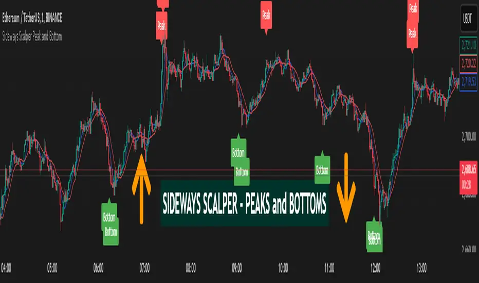
Strategy: Candlestick Wick Analysis with Volume Conditions
This strategy focuses on analyzing the wicks (or shadows) of candlesticks to identify potential trading opportunities based on candlestick structure and volume. Based on these criteria, it places stop orders at the extremities of the wicks when certain conditions are met, thus increasing the chances of capturing significant price movements.
Trading Criteria
Volume Conditions:
The strategy checks if the volume of the current candle is higher than that of the previous three candles. This ensures that the observed price movement is supported by significant volume, increasing the probability that the price will continue in the same direction.
Wick Analysis:
Upper Wick:
If the upper wick of a candle represents more than 90% of its body size and is longer than the lower wick, this indicates that the price tested a resistance level before pulling back.
Order Placement: In this case, a Buy Stop order is placed at the upper extremity of the wick. This means that if the price rises back to this level, the order will be triggered, and the trader will take a buy position.
SL Management: A stop-loss is then placed below the lowest point of the same candle. This protects the trader by limiting losses if the price falls back after the order is triggered.
Lower Wick:
If the lower wick of a candle is longer than the upper wick and represents more than 90% of its body size, this indicates that the price tested a support level before rising.
Order Placement: In this case, a Sell Stop order is placed at the lower extremity of the wick. Thus, if the price drops back to this level, the order will be triggered, and the trader will take a sell position.
SL Management: A stop-loss is then placed above the highest point of the same candle. This ensures risk management by limiting losses if the price rebounds upward after the order is triggered.
Strategy Advantages
Responsiveness to Price Movements: The strategy is designed to detect significant price movements based on the market's reaction around support and resistance levels. By placing stop orders directly at the wick extremities, it allows capturing strong movements in the direction indicated by the candles.
Securing Positions: Using stop-losses positioned just above or below key levels (wicks) provides better risk management. If the market doesn't move as expected, the position is automatically closed with a limited loss.
Clear Visual Indicators: Symbols are displayed on the chart at the points where orders have been placed, making it easier to understand trading decisions. This helps to quickly identify the support or resistance levels tested by the price, as well as potential entry points.
Conclusion
The strategy is based on the idea that large wicks signal areas where buyers or sellers have tested significant price levels before temporarily retreating. By placing stop orders at the extremities of these wicks, the strategy allows capturing price movements when they confirm, while limiting risks through strategically placed stop-losses. It thus offers a balanced approach between capturing potential profit and managing risk.
This description emphasizes the idea of capturing significant market movements with stop orders while providing a clear explanation of the logic and risk management. It’s tailored for publication on TradingView and highlights the robustness of the strategy.
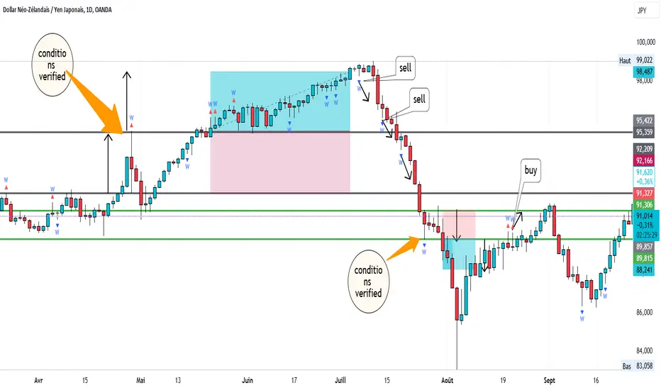
Cracking Cryptocurrency - Bottom FeederThe Bottom Feeder
The Bottom Feeder is designed to algorithmically detect significantly oversold conditions in price that represent profitable buying opportunities. Combining this with it’s unique Stop and Target System, the Bottom Feeder is designed to return consistent return with minimal draw down. Whether used as a Market Bottom Detector or as a system for executing safe, profitable mean reversion trades, the Bottom Feeder is a powerful tool in any trader’s arsenal.
Bottom Feeder was designed to be used on BTCUSD , however it is also effective on other USD/USDT pairs. One will have to check the individual pair they wish to trade with the Strategy Tester to simulate performance.
Options
Let’s go through the input options one by one, so that you are able to comfortably navigate all that this indicator has to offer. The link below will display a picture of the layout of the settings for your convenience.
For the sake of simplicity, let’s note now that all settings marked **Conservative Mode** will not work in Aggressive Mode.
Mode: Determines how aggressively Bottom Feeder generates a buy signal. In Conservative Mode, trades can only be opened once per candle and the stop and target will update as new signals appear. In Aggressive Mode, a separate trade is opened each time Bottom Feeder signals, which may be multiple times within one Daily candle.
Plot Target and Stop Loss: Toggles on/off the visualized take profit and stop losses on the chart.
**Conservative Mode** TP Multiplier: This is an input box, it requires a float value. That is, it can accept either a whole number integer or a number with a decimal. This number will determine your Take Profit target. It will take whatever number is entered into this box and multiply the Average True Range against it to determine your Take Profit.
**Conservative Mode** SL Multiplier: See above - this will modify your Stop Loss Value.
**Conservative Mode** Average or Median True Range: This is a drop-down option, the two options are Average True Range or Median True Range. If Average True Range is selected, then this indicator will use the Average True Range calculation, that is, the average of a historical set of True Range values to determine the Average True Range value for Target and Stop Loss calculation. If Median True Range is selected, it will not take an average and will instead take the Median value of your historical look back period.
**Conservative Mode** True Range Length: This is an input that requires an integer. This will represent your historical look back period for Average/Median True Range calculation.
**Conservative Mode** True Range Smoothing: This is a drop-down with the following options: Exponential Moving Average ( EMA ), Simple Moving Average ( SMA ), Weighted Moving Average ( WMA ), Relative Moving Average (RMA). This will determine the smoothing type for calculating the Average True Range if it is selected. Note: if Median True Range is selected above, this option will not have any effect as there is no smoothing for a Median value.
**Conservative Mode** Custom True Range Value?: This is a true/false option that is false by default. If enabled, it will override the Average/Median True Range calculation in favor of a users custom True Range value to be input below.
**Conservative Mode** Custom True Range Value: This is an input box that requires a float value. If Custom True Range is enabled this is where a user will input their desired custom True Range value for Target and Stop Loss calculation.
Stop and Target Description
Because Bottom Feeder is designed only to scalp the various market bottoms that can appear over time in the market and not to identify trends or to trade ranges, it’s imperative that the indicator notify us not just to when to enter our trades, but when to exit! In the service of that, CC Bottom Feeder has a built in Stop and Target system that tracks and displays the stop loss and take profit levels of each individual open trade, whether in Aggressive or Conservative Mode.
Conservative Mode Targeting: In Conservative Mode, Bottom Feeder signals are aggregated into a compound trade. The signal will appear as a green label pointing up below a candle, and will appear upon a candle close. If Bottom Feeder then generates another signal the stop loss and target price will be updated. The process will continue until the aggregated trade completes in either direction. On a trade with multiple signals, a larger position is slowly entered into upon each buy signal.
Aggressive Mode Targeting: In Aggressive Mode, Bottom Feeder signals are individually displayed as they are generated, regardless of how many signals are generated on any single candle. If Bottom Feeder continues to signal, each individual open trade will have their own stop loss and target that will be displayed on the chart until the individual trade completes in either direction. As opposed to a large compound position, aggressive mode represents a higher number of independent signals with their own stop and target levels.
Stop losses and targets are designed to be hard, not soft. That is, they are intended to be stop market orders, not mental stop losses. If price wicks through the target or stop, it will activate.
Algorithm Predator - ProAlgorithm Predator - Pro: Advanced Multi-Agent Reinforcement Learning Trading System
Algorithm Predator - Pro combines four specialized market microstructure agents with a state-of-the-art reinforcement learning framework . Unlike traditional indicator mashups, this system implements genuine machine learning to automatically discover which detection strategies work best in current market conditions and adapts continuously without manual intervention.
Core Innovation: Rather than forcing traders to interpret conflicting signals, this system uses 15 different multi-armed bandit algorithms and a full reinforcement learning stack (Q-Learning, TD(λ) with eligibility traces, and Policy Gradient with REINFORCE) to learn optimal agent selection policies. The result is a self-improving system that gets smarter with every trade.
Target Users: Swing traders, day traders, and algorithmic traders seeking systematic signal generation with mathematical rigor. Suitable for stocks, forex, crypto, and futures on liquid instruments (>100k daily volume).
Why These Components Are Combined
The Fundamental Problem
No single indicator works consistently across all market regimes. What works in trending markets fails in ranging conditions. Traditional solutions force traders to manually switch indicators (slow, error-prone) or interpret all signals simultaneously (cognitive overload).
This system solves the problem through automated meta-learning: Deploy multiple specialized agents designed for specific market microstructure conditions, then use reinforcement learning to discover which agent (or combination) performs best in real-time.
Why These Specific Four Agents?
The four agents provide orthogonal failure mode coverage —each agent's weakness is another's strength:
Spoofing Detector - Optimal in consolidation/manipulation; fails in trending markets (hedged by Exhaustion Detector)
Exhaustion Detector - Optimal at trend climax; fails in range-bound markets (hedged by Liquidity Void)
Liquidity Void - Optimal pre-breakout compression; fails in established trends (hedged by Mean Reversion)
Mean Reversion - Optimal in low volatility; fails in strong trends (hedged by Spoofing Detector)
This creates complete market state coverage where at least one agent should perform well in any condition. The bandit system identifies which one without human intervention.
Why Reinforcement Learning vs. Simple Voting?
Traditional consensus systems have fatal flaws: equal weighting assumes all agents are equally reliable (false), static thresholds don't adapt, and no learning means past mistakes repeat indefinitely.
Reinforcement learning solves this through the exploration-exploitation tradeoff: Continuously test underused agents (exploration) while primarily relying on proven winners (exploitation). Over time, the system builds a probability distribution over agent quality reflecting actual market performance.
Mathematical Foundation: Multi-armed bandit problem from probability theory, where each agent is an "arm" with unknown reward distribution. The goal is to maximize cumulative reward while efficiently learning each arm's true quality.
The Four Trading Agents: Technical Explanation
Agent 1: 🎭 Spoofing Detector (Institutional Manipulation Detection)
Theoretical Basis: Market microstructure theory on order flow toxicity and information asymmetry. Based on research by Easley, López de Prado, and O'Hara on high-frequency trading manipulation.
What It Detects:
1. Iceberg Orders (Hidden Liquidity Absorption)
Method: Monitors volume spikes (>2.5× 20-period average) with minimal price movement (<0.3× ATR)
Formula: score += (close > open ? -2.5 : 2.5) when volume > vol_avg × 2.5 AND abs(close - open) / ATR < 0.3
Interpretation: Large volume without price movement indicates institutional absorption (buying) or distribution (selling) using hidden orders
Signal Logic: Contrarian—fade false breakouts caused by institutional manipulation
2. Spoofing Patterns (Fake Liquidity via Layering)
Method: Analyzes candlestick wick-to-body ratios during volume spikes
Formula: if upper_wick > body × 2 AND volume_spike: score += 2.0
Mechanism: Spoofing creates large wicks (orders pulled before execution) with volume evidence
Signal Logic: Wick direction indicates trapped participants; trade against the failed move
3. Post-Manipulation Reversals
Method: Tracks volume decay after manipulation events
Formula: if volume > vol_avg × 3 AND volume / volume < 0.3: score += (close > open ? -1.5 : 1.5)
Interpretation: Sharp volume drop after manipulation indicates exhaustion of manipulative orders
Why It Works: Institutional manipulation creates detectable microstructure anomalies. While retail traders see "mysterious reversals," this agent quantifies the order flow patterns causing them.
Parameter: i_spoof (sensitivity 0.5-2.0) - Controls detection threshold
Best Markets: Consolidations before breakouts, London/NY overlap windows, stocks with institutional ownership >70%
Agent 2: ⚡ Exhaustion Detector (Momentum Failure Analysis)
Theoretical Basis: Technical analysis divergence theory combined with VPIN reversals from market microstructure literature.
What It Detects:
1. Price-RSI Divergence (Momentum Deceleration)
Method: Compares 5-bar price ROC against RSI change
Formula: if price_roc > 5% AND rsi_current < rsi : score += 1.8
Mathematics: Second derivative detecting inflection points
Signal Logic: When price makes higher highs but momentum makes lower highs, expect mean reversion
2. Volume Exhaustion (Buying/Selling Climax)
Method: Identifies strong price moves (>5% ROC) with declining volume (<-20% volume ROC)
Formula: if price_roc > 5 AND vol_roc < -20: score += 2.5
Interpretation: Price extension without volume support indicates retail chasing while institutions exit
3. Momentum Deceleration (Acceleration Analysis)
Method: Compares recent 3-bar momentum to prior 3-bar momentum
Formula: deceleration = abs(mom1) < abs(mom2) × 0.5 where momentum significant (> ATR)
Signal Logic: When rate of price change decelerates significantly, anticipate directional shift
Why It Works: Momentum is lagging, but momentum divergence is leading. By comparing momentum's rate of change to price, this agent detects "weakening conviction" before reversals become obvious.
Parameter: i_momentum (sensitivity 0.5-2.0)
Best Markets: Strong trends reaching climax, parabolic moves, instruments with high retail participation
Agent 3: 💧 Liquidity Void Detector (Breakout Anticipation)
Theoretical Basis: Market liquidity theory and order book dynamics. Based on research into "liquidity holes" and volatility compression preceding expansion.
What It Detects:
1. Bollinger Band Squeeze (Volatility Compression)
Method: Monitors Bollinger Band width relative to 50-period average
Formula: bb_width = (upper_band - lower_band) / middle_band; triggers when < 0.6× average
Mathematical Foundation: Regression to the mean—low volatility precedes high volatility
Signal Logic: When volatility compresses AND cumulative delta shows directional bias, anticipate breakout
2. Volume Profile Gaps (Thin Liquidity Zones)
Method: Identifies sharp volume transitions indicating few limit orders
Formula: if volume < vol_avg × 0.5 AND volume < vol_avg × 0.5 AND volume > vol_avg × 1.5
Interpretation: Sudden volume drop after spike indicates price moved through order book to low-opposition area
Signal Logic: Price accelerates through low-liquidity zones
3. Stop Hunts (Liquidity Grabs Before Reversals)
Method: Detects new 20-bar highs/lows with immediate reversal and rejection wick
Formula: if new_high AND close < high - (high - low) × 0.6: score += 3.0
Mechanism: Market makers push price to trigger stop-loss clusters, then reverse
Signal Logic: Enter reversal after stop-hunt completes
Why It Works: Order book theory shows price moves fastest through zones with minimal liquidity. By identifying these zones before major moves, this agent provides early entry for high-reward breakouts.
Parameter: i_liquidity (sensitivity 0.5-2.0)
Best Markets: Range-bound pre-breakout setups, volatility compression zones, instruments prone to gap moves
Agent 4: 📊 Mean Reversion (Statistical Arbitrage Engine)
Theoretical Basis: Statistical arbitrage theory, Ornstein-Uhlenbeck mean-reverting processes, and pairs trading methodology applied to single instruments.
What It Detects:
1. Z-Score Extremes (Standard Deviation Analysis)
Method: Calculates price distance from 20-period and 50-period SMAs in standard deviation units
Formula: zscore_20 = (close - SMA20) / StdDev(50)
Statistical Interpretation: Z-score >2.0 means price is 2 standard deviations above mean (97.5th percentile)
Trigger Logic: if abs(zscore_20) > 2.0: score += zscore_20 > 0 ? -1.5 : 1.5 (fade extremes)
2. Ornstein-Uhlenbeck Process (Mean-Reverting Stochastic Model)
Method: Models price as mean-reverting stochastic process: dx = θ(μ - x)dt + σdW
Implementation: Calculates spread = close - SMA20, then z-score of spread vs. spread distribution
Formula: ou_signal = (spread - spread_mean) / spread_std
Interpretation: Measures "tension" pulling price back to equilibrium
3. Correlation Breakdown (Regime Change Detection)
Method: Compares 50-period price-volume correlation to 10-period correlation
Formula: corr_breakdown = abs(typical_corr - recent_corr) > 0.5
Enhancement: if corr_breakdown AND abs(zscore_20) > 1.0: score += zscore_20 > 0 ? -1.2 : 1.2
Why It Works: Mean reversion is the oldest quantitative strategy (1970s pairs trading at Morgan Stanley). While simple, it remains effective because markets exhibit periodic equilibrium-seeking behavior. This agent applies rigorous statistical testing to identify when mean reversion probability is highest.
Parameter: i_statarb (sensitivity 0.5-2.0)
Best Markets: Range-bound instruments, low-volatility periods (VIX <15), algo-dominated markets (forex majors, index futures)
Multi-Armed Bandit System: 15 Algorithms Explained
What Is a Multi-Armed Bandit Problem?
Origin: Named after slot machines ("one-armed bandits"). Imagine facing multiple slot machines, each with unknown payout rates. How do you maximize winnings?
Formal Definition: K arms (agents), each with unknown reward distribution with mean μᵢ. Goal: Maximize cumulative reward over T trials. Challenge: Balance exploration (trying uncertain arms to learn quality) vs. exploitation (using known-best arm for immediate reward).
Trading Application: Each agent is an "arm." After each trade, receive reward (P&L). Must decide which agent to trust for next signal.
Algorithm Categories
Bayesian Approaches (probabilistic, optimal for stationary environments):
Thompson Sampling
Bootstrapped Thompson Sampling
Discounted Thompson Sampling
Frequentist Approaches (confidence intervals, deterministic):
UCB1
UCB1-Tuned
KL-UCB
SW-UCB (Sliding Window)
D-UCB (Discounted)
Adversarial Approaches (robust to non-stationary environments):
EXP3-IX
Hedge
FPL-Gumbel
Reinforcement Learning Approaches (leverage learned state-action values):
Q-Values (from Q-Learning)
Policy Network (from Policy Gradient)
Simple Baseline:
Epsilon-Greedy
Softmax
Key Algorithm Details
Thompson Sampling (DEFAULT - RECOMMENDED)
Theoretical Foundation: Bayesian decision theory with conjugate priors. Published by Thompson (1933), rediscovered for bandits by Chapelle & Li (2011).
How It Works:
Model each agent's reward distribution as Beta(α, β) where α = wins, β = losses
Each step, sample from each agent's beta distribution: θᵢ ~ Beta(αᵢ, βᵢ)
Select agent with highest sample: argmaxᵢ θᵢ
Update winner's distribution after observing outcome
Mathematical Properties:
Optimality: Achieves logarithmic regret O(K log T) (proven optimal)
Bayesian: Maintains probability distribution over true arm means
Automatic Balance: High uncertainty → more exploration; high certainty → exploitation
⚠️ CRITICAL APPROXIMATION: This is a pseudo-random approximation of true Thompson Sampling. True implementation requires random number generation from beta distributions, which Pine Script doesn't provide. This version uses Box-Muller transform with market data (price/volume decimal digits) as entropy source. While not mathematically pure, it maintains core exploration-exploitation balance and learns agent preferences effectively.
When To Use: Best all-around choice. Handles non-stationary markets reasonably well, balances exploration naturally, highly sample-efficient.
UCB1 (Upper Confidence Bound)
Formula: UCB_i = reward_mean_i + sqrt(2 × ln(total_pulls) / pulls_i)
Interpretation: First term (exploitation) + second term (exploration bonus for less-tested arms)
Mathematical Properties:
Deterministic : Always selects same arm given same state
Regret Bound: O(K log T) — same optimality as Thompson Sampling
Interpretable: Can visualize confidence intervals
When To Use: Prefer deterministic behavior, want to visualize uncertainty, stable markets
EXP3-IX (Exponential Weights - Adversarial)
Theoretical Foundation: Adversarial bandit algorithm. Assumes environment may be actively hostile (worst-case analysis).
How It Works:
Maintain exponential weights: w_i = exp(η × cumulative_reward_i)
Select agent with probability proportional to weights: p_i = (1-γ)w_i/Σw_j + γ/K
After outcome, update with importance weighting: estimated_reward = observed_reward / p_i
Mathematical Properties:
Adversarial Regret: O(sqrt(TK log K)) even if environment is adversarial
No Assumptions: Doesn't assume stationary or stochastic reward distributions
Robust: Works even when optimal arm changes continuously
When To Use: Extreme non-stationarity, don't trust reward distribution assumptions, want robustness over efficiency
KL-UCB (Kullback-Leibler Upper Confidence Bound)
Theoretical Foundation: Uses KL-divergence instead of Hoeffding bounds. Tighter confidence intervals.
Formula (conceptual): Find largest q such that: n × KL(p||q) ≤ ln(t) + 3×ln(ln(t))
Mathematical Properties:
Tighter Bounds: KL-divergence adapts to reward distribution shape
Asymptotically Optimal: Better constant factors than UCB1
Computationally Intensive: Requires iterative binary search (15 iterations)
When To Use: Maximum sample efficiency needed, willing to pay computational cost, long-term trading (>500 bars)
Q-Values & Policy Network (RL-Based Selection)
Unique Feature: Instead of treating agents as black boxes with scalar rewards, these algorithms leverage the full RL state representation .
Q-Values Selection:
Uses learned Q-values: Q(state, agent_i) from Q-Learning
Selects agent via softmax over Q-values for current market state
Advantage: Selects based on state-conditional quality (which agent works best in THIS market state)
Policy Network Selection:
Uses neural network policy: π(agent | state, θ) from Policy Gradient
Direct policy over agents given market features
Advantage: Can learn non-linear relationships between market features and agent quality
When To Use: After 200+ RL updates (Q-Values) or 500+ updates (Policy Network) when models converged
Machine Learning & Reinforcement Learning Stack
Why Both Bandits AND Reinforcement Learning?
Critical Distinction:
Bandits treat agents as contextless black boxes: "Agent 2 has 60% win rate"
Reinforcement Learning adds state context: "Agent 2 has 60% win rate WHEN trend_score > 2 and RSI < 40"
Power of Combination: Bandits provide fast initial learning with minimal assumptions. RL provides state-dependent policies for superior long-term performance.
Component 1: Q-Learning (Value-Based RL)
Algorithm: Temporal Difference Learning with Bellman equation.
State Space: 54 discrete states formed from:
trend_state = {0: bearish, 1: neutral, 2: bullish} (3 values)
volatility_state = {0: low, 1: normal, 2: high} (3 values)
RSI_state = {0: oversold, 1: neutral, 2: overbought} (3 values)
volume_state = {0: low, 1: high} (2 values)
Total states: 3 × 3 × 3 × 2 = 54 states
Action Space: 5 actions (No trade, Agent 1, Agent 2, Agent 3, Agent 4)
Total state-action pairs: 54 × 5 = 270 Q-values
Bellman Equation:
Q(s,a) ← Q(s,a) + α ×
Parameters:
α (learning rate): 0.01-0.50, default 0.10 - Controls step size for updates
γ (discount factor): 0.80-0.99, default 0.95 - Values future rewards
ε (exploration): 0.01-0.30, default 0.10 - Probability of random action
Update Mechanism:
Position opens with state s, action a (selected agent)
Every bar position is open: Calculate floating P&L → scale to reward
Perform online TD update
When position closes: Perform terminal update with final reward
Gradient Clipping: TD errors clipped to ; Q-values clipped to for stability.
Why It Works: Q-Learning learns "quality" of each agent in each market state through trial and error. Over time, builds complete state-action value function enabling optimal state-dependent agent selection.
Component 2: TD(λ) Learning (Temporal Difference with Eligibility Traces)
Enhancement Over Basic Q-Learning: Credit assignment across multiple time steps.
The Problem TD(λ) Solves:
Position opens at t=0
Market moves favorably at t=3
Position closes at t=8
Question: Which earlier decisions contributed to success?
Basic Q-Learning: Only updates Q(s₈, a₈) ← reward
TD(λ): Updates ALL visited state-action pairs with decayed credit
Eligibility Trace Formula:
e(s,a) ← γ × λ × e(s,a) for all s,a (decay all traces)
e(s_current, a_current) ← 1 (reset current trace)
Q(s,a) ← Q(s,a) + α × TD_error × e(s,a) (update all with trace weight)
Lambda Parameter (λ): 0.5-0.99, default 0.90
λ=0: Pure 1-step TD (only immediate next state)
λ=1: Full Monte Carlo (entire episode)
λ=0.9: Balance (recommended)
Why Superior: Dramatically faster learning for multi-step tasks. Q-Learning requires many episodes to propagate rewards backwards; TD(λ) does it in one.
Component 3: Policy Gradient (REINFORCE with Baseline)
Paradigm Shift: Instead of learning value function Q(s,a), directly learn policy π(a|s).
Policy Network Architecture:
Input: 12 market features
Hidden: None (linear policy)
Output: 5 actions (softmax distribution)
Total parameters: 12 features × 5 actions + 5 biases = 65 parameters
Feature Set (12 Features):
Price Z-score (close - SMA20) / ATR
Volume ratio (volume / vol_avg - 1)
RSI deviation (RSI - 50) / 50
Bollinger width ratio
Trend score / 4 (normalized)
VWAP deviation
5-bar price ROC
5-bar volume ROC
Range/ATR ratio - 1
Price-volume correlation (20-period)
Volatility ratio (ATR / ATR_avg - 1)
EMA50 deviation
REINFORCE Update Rule:
θ ← θ + α × ∇log π(a|s) × advantage
where advantage = reward - baseline (variance reduction)
Why Baseline? Raw rewards have high variance. Subtracting baseline (running average) centers rewards around zero, reducing gradient variance by 50-70%.
Learning Rate: 0.001-0.100, default 0.010 (much lower than Q-Learning because policy gradients have high variance)
Why Policy Gradient?
Handles 12 continuous features directly (Q-Learning requires discretization)
Naturally maintains exploration through probability distribution
Can converge to stochastic optimal policy
Component 4: Ensemble Meta-Learner (Stacking)
Architecture: Level-1 meta-learner combines Level-0 base learners (Q-Learning, TD(λ), Policy Gradient).
Three Meta-Learning Algorithms:
1. Simple Average (Baseline)
Final_prediction = (Q_prediction + TD_prediction + Policy_prediction) / 3
2. Weighted Vote (Reward-Based)
weight_i ← 0.95 × weight_i + 0.05 × (reward_i + 1)
3. Adaptive Weighting (Gradient-Based) — RECOMMENDED
Loss Function: L = (y_true - ŷ_ensemble)²
Gradient: ∂L/∂weight_i = -2 × (y_true - ŷ_ensemble) × agent_contribution_i
Updates weights via gradient descent with clipping and normalization
Why It Works: Unlike simple averaging, meta-learner discovers which base learner is most reliable in current regime. If Policy Gradient excels in trending markets while Q-Learning excels in ranging, meta-learner learns these patterns and weights accordingly.
Feature Importance Tracking
Purpose: Identify which of 12 features contribute most to successful predictions.
Update Rule: importance_i ← 0.95 × importance_i + 0.05 × |feature_i × reward|
Use Cases:
Feature selection: Drop low-importance features
Market regime detection: Importance shifts reveal regime changes
Agent tuning: If VWAP deviation has high importance, consider boosting agents using VWAP
RL Position Tracking System
Critical Innovation: Proper reinforcement learning requires tracking which decisions led to outcomes.
State Tracking (When Signal Validates):
active_rl_state ← current_market_state (0-53)
active_rl_action ← selected_agent (1-4)
active_rl_entry ← entry_price
active_rl_direction ← 1 (long) or -1 (short)
active_rl_bar ← current_bar_index
Online Updates (Every Bar Position Open):
floating_pnl = (close - entry) / entry × direction
reward = floating_pnl × 10 (scale to meaningful range)
reward = clip(reward, -5.0, 5.0)
Update Q-Learning, TD(λ), and Policy Gradient
Terminal Update (Position Close):
Final Q-Learning update (no next Q-value, terminal state)
Update meta-learner with final result
Update agent memory
Clear position tracking
Exit Conditions:
Time-based: ≥3 bars held (minimum hold period)
Stop-loss: 1.5% adverse move
Take-profit: 2.0% favorable move
Market Microstructure Filters
Why Microstructure Matters
Traditional technical analysis assumes fair, efficient markets. Reality: Markets have friction, manipulation, and information asymmetry. Microstructure filters detect when market structure indicates adverse conditions.
Filter 1: VPIN (Volume-Synchronized Probability of Informed Trading)
Theoretical Foundation: Easley, López de Prado, & O'Hara (2012). "Flow Toxicity and Liquidity in a High-Frequency World."
What It Measures: Probability that current order flow is "toxic" (informed traders with private information).
Calculation:
Classify volume as buy or sell (close > close = buy volume)
Calculate imbalance over 20 bars: VPIN = |Σ buy_volume - Σ sell_volume| / Σ total_volume
Compare to moving average: toxic = VPIN > VPIN_MA(20) × sensitivity
Interpretation:
VPIN < 0.3: Normal flow (uninformed retail)
VPIN 0.3-0.4: Elevated (smart money active)
VPIN > 0.4: Toxic flow (informed institutions dominant)
Filter Logic:
Block LONG when: VPIN toxic AND price rising (don't buy into institutional distribution)
Block SHORT when: VPIN toxic AND price falling (don't sell into institutional accumulation)
Adaptive Threshold: If VPIN toxic frequently, relax threshold; if rarely toxic, tighten threshold. Bounded .
Filter 2: Toxicity (Kyle's Lambda Approximation)
Theoretical Foundation: Kyle (1985). "Continuous Auctions and Insider Trading."
What It Measures: Price impact per unit volume — market depth and informed trading.
Calculation:
price_impact = (close - close ) / sqrt(Σ volume over 10 bars)
impact_zscore = (price_impact - impact_mean) / impact_std
toxicity = abs(impact_zscore)
Interpretation:
Low toxicity (<1.0): Deep liquid market, large orders absorbed easily
High toxicity (>2.0): Thin market or informed trading
Filter Logic: Block ALL SIGNALS when toxicity > threshold. Most dangerous when price breaks from VWAP with high toxicity.
Filter 3: Regime Filter (Counter-Trend Protection)
Purpose: Prevent counter-trend trades during strong trends.
Trend Scoring:
trend_score = 0
trend_score += close > EMA8 ? +1 : -1
trend_score += EMA8 > EMA21 ? +1 : -1
trend_score += EMA21 > EMA50 ? +1 : -1
trend_score += close > EMA200 ? +1 : -1
Range:
Regime Classification:
Strong Bull: trend_score ≥ +3 → Block all SHORT signals
Strong Bear: trend_score ≤ -3 → Block all LONG signals
Neutral: -2 ≤ trend_score ≤ +2 → Allow both directions
Filter 4: Liquidity Boost (Signal Enhancer)
Unique: Unlike other filters (which block), this amplifies signals during low liquidity.
Logic: if volume < vol_avg × 0.7: agent_scores × 1.2
Why It Works: Low liquidity often precedes explosive moves (breakouts). By increasing agent sensitivity during compression, system catches pre-breakout signals earlier.
Technical Implementation & Approximations
⚠️ Critical Approximations Required by Pine Script
1. Thompson Sampling: Pseudo-Random Beta Distribution
Academic Standard: True random sampling from beta distributions using cryptographic RNG
This Implementation: Box-Muller transform for normal distribution using market data (price/volume decimal digits) as entropy source, then scale to beta distribution mean/variance
Impact: Not cryptographically random, may have subtle biases in specific price ranges, but maintains correct mean and approximate variance. Sufficient for bandit agent selection.
2. VPIN: Simplified Volume Classification
Academic Standard: Lee-Ready algorithm or exchange-provided aggressor flags with tick-by-tick data
This Implementation: Bar-based classification: if close > close : buy_volume += volume
Impact: 10-15% precision loss. Works well in directional markets, misclassifies in choppy conditions. Still captures order flow imbalance signal.
3. Policy Gradient: Simplified Per-Action Updates
Academic Standard: Full softmax gradient updating all actions (selected action UP, others DOWN proportionally)
This Implementation: Only updates selected action's weights
Impact: Valid approximation for small action spaces (5 actions). Slower convergence than full softmax but still learns optimal policy.
4. Kyle's Lambda: Simplified Price Impact
Academic Standard: Regression over multiple time scales with signed order flow
This Implementation: price_impact = Δprice_10 / sqrt(Σvolume_10); z_score calculation
Impact: 15-20% precision loss. No proper signed order flow. Still detects informed trading signals at extremes (>2σ).
5. Other Simplifications:
Hawkes Process: Fixed exponential decay (0.9) not MLE-optimized
Entropy: Ratio approximation not true Shannon entropy H(X) = -Σ p(x)·log₂(p(x))
Feature Engineering: 12 features vs. potential 100+ with polynomial interactions
RL Hybrid Updates: Both online and terminal (non-standard but empirically effective)
Overall Precision Loss Estimate: 10-15% compared to academic implementations with institutional data feeds.
Practical Trade-off: For retail trading with OHLCV data, these approximations provide 90%+ of the edge while maintaining full transparency, zero latency, no external dependencies, and runs on any TradingView plan.
How to Use: Practical Guide
Initial Setup (5 Minutes)
Select Trading Mode: Start with "Balanced" for most users
Enable ML/RL System: Toggle to TRUE, select "Full Stack" ML Mode
Bandit Configuration: Algorithm: "Thompson Sampling", Mode: "Switch" or "Blend"
Microstructure Filters: Enable all four filters, enable "Adaptive Microstructure Thresholds"
Visual Settings: Enable dashboard (Top Right), enable all chart visuals
Learning Phase (First 50-100 Signals)
What To Monitor:
Agent Performance Table: Watch win rates develop (target >55%)
Bandit Weights: Should diverge from uniform (0.25 each) after 20-30 signals
RL Core Metrics: "RL Updates" should increase when position open
Filter Status: "Blocked" count indicates filter activity
Optimization Tips:
Too few signals: Lower min_confidence to 0.25, increase agent sensitivities to 1.1-1.2
Too many signals: Raise min_confidence to 0.35-0.40, decrease agent sensitivities to 0.8-0.9
One agent dominates (>70%): Consider "Lock Agent" feature
Signal Interpretation
Dashboard Signal Status:
⚪ WAITING FOR SIGNAL: No agent signaling
⏳ ANALYZING...: Agent signaling but not confirmed
🟡 CONFIRMING 2/3: Building confirmation (2 of 3 bars)
🟢 LONG ACTIVE : Validated long entry
🔴 SHORT ACTIVE : Validated short entry
Kill Zone Boxes: Entry price (triangle marker), Take Profit (Entry + 2.5× ATR), Stop Loss (Entry - 1.5× ATR). Risk:Reward = 1:1.67
Risk Management
Position Sizing:
Risk per trade = 1-2% of capital
Position size = (Capital × Risk%) / (Entry - StopLoss)
Stop-Loss Placement:
Initial: Entry ± 1.5× ATR (shown in kill zone)
Trailing: After 1:1 R:R achieved, move stop to breakeven
Take-Profit Strategy:
TP1 (2.5× ATR): Take 50% off
TP2 (Runner): Trail stop at 1× ATR or use opposite signal as exit
Memory Persistence
Why Save Memory: Every chart reload resets the system. Saving learned parameters preserves weeks of learning.
When To Save: After 200+ signals when agent weights stabilize
What To Save: From Memory Export panel, copy all alpha/beta/weight values and adaptive thresholds
How To Restore: Enable "Restore From Saved State", input all values into corresponding fields
What Makes This Original
Innovation 1: Genuine Multi-Armed Bandit Framework
This implements 15 mathematically rigorous bandit algorithms from academic literature (Thompson Sampling from Chapelle & Li 2011, UCB family from Auer et al. 2002, EXP3 from Auer et al. 2002, KL-UCB from Garivier & Cappé 2011). Each algorithm maintains proper state, updates according to proven theory, and converges to optimal behavior. This is real learning, not superficial parameter changes.
Innovation 2: Full Reinforcement Learning Stack
Beyond bandits learning which agent works best globally, RL learns which agent works best in each market state. After 500+ positions, system builds 54-state × 5-action value function (270 learned parameters) capturing context-dependent agent quality.
Innovation 3: Market Microstructure Integration
Combines retail technical analysis with institutional-grade microstructure metrics: VPIN from Easley, López de Prado, O'Hara (2012), Kyle's Lambda from Kyle (1985), Hawkes Processes from Hawkes (1971). These detect informed trading, manipulation, and liquidity dynamics invisible to technical analysis.
Innovation 4: Adaptive Threshold System
Dynamic quantile-based thresholds: Maintains histogram of each agent's score distribution (24 bins, exponentially decayed), calculates 80th percentile threshold from histogram. Agent triggers only when score exceeds its own learned quantile. Proper non-parametric density estimation automatically adapts to instrument volatility, agent behavior shifts, and market regime changes.
Innovation 5: Episodic Memory with Transfer Learning
Dual-layer architecture: Short-term memory (last 20 trades, fast adaptation) + Long-term memory (condensed episodes, historical patterns). Transfer mechanism consolidates knowledge when STM reaches threshold. Mimics hippocampus → neocortex consolidation in human memory.
Limitations & Disclaimers
General Limitations
No Predictive Guarantee: Pattern recognition ≠ prediction. Past performance ≠ future results.
Learning Period Required: Minimum 50-100 bars for reliable statistics. Initial performance may be suboptimal.
Overfitting Risk: System learns patterns in historical data. May not generalize to unprecedented conditions.
Approximation Limitations: See technical implementation section (10-15% precision loss vs. academic standards)
Single-Instrument Limitation: No multi-asset correlation, sector context, or VIX integration.
Forward-Looking Bias Disclaimer
CRITICAL TRANSPARENCY: The RL system uses an 8-bar forward-looking window for reward calculation.
What This Means: System learns from rewards incorporating future price information (bars 101-108 relative to entry at bar 100).
Why Acceptable:
✅ Signals do NOT look ahead: Entry decisions use only data ≤ entry bar
✅ Learning only: Forward data used for optimization, not signal generation
✅ Real-time mirrors backtest: In live trading, system learns identically
⚠️ Implication: Dashboard "Agent Win%" reflects this 8-bar evaluation. Real-time performance may differ slightly if positions held longer, slippage/fees not captured, or market microstructure changes.
Risk Warnings
No Guarantee of Profit: All trading involves risk of loss
System Failures: Bugs possible despite extensive testing
Market Conditions: Optimized for liquid markets (>100k daily volume). Performance degrades in illiquid instruments, major news events, flash crashes
Broker-Specific Issues: Execution slippage, commission/fees, overnight financing costs
Appropriate Use
This Indicator Is:
✅ Entry trigger system
✅ Risk management framework (stop/target)
✅ Adaptive agent selection engine
✅ Learning system that improves over time
This Indicator Is NOT:
❌ Complete trading strategy (requires position sizing, portfolio management)
❌ Replacement for fundamental analysis
❌ Guaranteed profit generator
❌ Suitable for complete beginners without training
Recommended Complementary Analysis: Market context (support/resistance), volume profile, fundamental catalysts, correlation with related instruments, broader market regime
Recommended Settings by Instrument
Stocks (Large Cap, >$1B):
Mode: Balanced | ML/RL: Enabled, Full Stack | Bandit: Thompson Sampling, Switch
Agent Sensitivity: Spoofing 1.0-1.2, Exhaustion 0.9-1.1, Liquidity 0.8-1.0, StatArb 1.1-1.3
Microstructure: All enabled, VPIN 1.2, Toxicity 1.5 | Timeframe: 15min-1H
Forex Majors (EURUSD, GBPUSD):
Mode: Balanced to Conservative | ML/RL: Enabled, Full Stack | Bandit: Thompson Sampling, Blend
Agent Sensitivity: Spoofing 0.8-1.0, Exhaustion 0.9-1.1, Liquidity 0.7-0.9, StatArb 1.2-1.5
Microstructure: All enabled, VPIN 1.0-1.1, Toxicity 1.3-1.5 | Timeframe: 5min-30min
Crypto (BTC, ETH):
Mode: Aggressive to Balanced | ML/RL: Enabled, Full Stack | Bandit: Thompson Sampling OR EXP3-IX
Agent Sensitivity: Spoofing 1.2-1.5, Exhaustion 1.1-1.3, Liquidity 1.2-1.5, StatArb 0.7-0.9
Microstructure: All enabled, VPIN 1.4-1.6, Toxicity 1.8-2.2 | Timeframe: 15min-4H
Futures (ES, NQ, CL):
Mode: Balanced | ML/RL: Enabled, Full Stack | Bandit: UCB1 or Thompson Sampling
Agent Sensitivity: All 1.0-1.2 (balanced)
Microstructure: All enabled, VPIN 1.1-1.3, Toxicity 1.4-1.6 | Timeframe: 5min-30min
Conclusion
Algorithm Predator - Pro synthesizes academic research from market microstructure theory, reinforcement learning, and multi-armed bandit algorithms. Unlike typical indicator mashups, this system implements 15 mathematically rigorous bandit algorithms, deploys a complete RL stack (Q-Learning, TD(λ), Policy Gradient), integrates institutional microstructure metrics (VPIN, Kyle's Lambda), adapts continuously through dual-layer memory and meta-learning, and provides full transparency on approximations and limitations.
The system is designed for serious algorithmic traders who understand that no indicator is perfect, but through proper machine learning, we can build systems that improve over time and adapt to changing markets without manual intervention.
Use responsibly. Risk disclosure applies. Past performance ≠ future results.
Taking you to school. — Dskyz, Trade with insight. Trade with anticipation.

Manifold Singularity EngineManifold Singularity Engine: Catastrophe Theory Detection Through Multi-Dimensional Topology Analysis
The Manifold Singularity Engine applies catastrophe theory from mathematical topology to multi-dimensional price space analysis, identifying potential reversal conditions by measuring manifold curvature, topological complexity, and fractal regime states. Unlike traditional reversal indicators that rely on price pattern recognition or momentum oscillators, this system reconstructs the underlying geometric surface (manifold) that price evolves upon and detects points where this topology undergoes catastrophic folding—mathematical singularities that correspond to forced directional changes in price dynamics.
The indicator combines three analytical frameworks: phase space reconstruction that embeds price data into a multi-dimensional coordinate system, catastrophe detection that measures when this embedded manifold reaches critical curvature thresholds indicating topology breaks, and Hurst exponent calculation that classifies the current fractal regime to adaptively weight detection sensitivity. This creates a geometry-based reversal detection system with visual feedback showing topology state, manifold distortion fields, and directional probability projections.
What Makes This Approach Different
Phase Space Embedding Construction
The core analytical method reconstructs price evolution as movement through a three-dimensional coordinate system rather than analyzing price as a one-dimensional time series. The system calculates normalized embedding coordinates: X = normalize(price_velocity, window) , Y = normalize(momentum_acceleration, window) , and Z = normalize(volume_weighted_returns, window) . These coordinates create a trajectory through phase space where price movement traces a path across a geometric surface—the market manifold.
This embedding approach differs fundamentally from traditional technical analysis by treating price not as a sequential data stream but as a dynamical system evolving on a curved surface in multi-dimensional space. The trajectory's geometric properties (curvature, complexity, folding) contain information about impending directional changes that single-dimension analysis cannot capture. When this manifold undergoes rapid topological deformation, price must respond with directional change—this is the mathematical basis for catastrophe detection.
Statistical normalization using z-score transformation (subtracting mean, dividing by standard deviation over a rolling window) ensures the coordinate system remains scale-invariant across different instruments and volatility regimes, allowing identical detection logic to function on forex, crypto, stocks, or indices without recalibration.
Catastrophe Score Calculation
The catastrophe detection formula implements a composite anomaly measurement combining multiple topology metrics: Catastrophe_Score = 0.45×Curvature_Percentile + 0.25×Complexity_Ratio + 0.20×Condition_Percentile + 0.10×Gradient_Percentile . Each component measures a distinct aspect of manifold distortion:
Curvature (κ) is computed using the discrete Laplacian operator: κ = √ , which measures how sharply the manifold surface bends at the current point. High curvature values indicate the surface is folding or developing a sharp corner—geometric precursors to catastrophic topology breaks. The Laplacian measures second derivatives (rate of change of rate of change), capturing acceleration in the trajectory's path through phase space.
Topological Complexity counts sign changes in the curvature field over the embedding window, measuring how chaotically the manifold twists and oscillates. A smooth, stable surface produces low complexity; a highly contorted, unstable surface produces high complexity. This metric detects when the geometric structure becomes informationally dense with multiple local extrema, suggesting an imminent topology simplification event (catastrophe).
Condition Number measures the Jacobian matrix's sensitivity: Condition = |Trace| / |Determinant|, where the Jacobian describes how small changes in price produce changes in the embedding coordinates. High condition numbers indicate numerical instability—points where the coordinate transformation becomes ill-conditioned, suggesting the manifold mapping is approaching a singularity.
Each metric is converted to percentile rank within a rolling window, then combined using weighted sum. The percentile transformation creates adaptive thresholds that automatically adjust to each instrument's characteristic topology without manual recalibration. The resulting 0-100% catastrophe score represents the current bar's position in the distribution of historical manifold distortion—values above the threshold (default 65%) indicate statistically extreme topology states where reversals become geometrically probable.
This multi-metric ensemble approach prevents false signals from isolated anomalies: all four geometric features must simultaneously indicate distortion for a high catastrophe score, ensuring only true manifold breaks trigger detection.
Hurst Exponent Regime Classification
The Hurst exponent calculation implements rescaled range (R/S) analysis to measure the fractal dimension of price returns: H = log(R/S) / log(n) , where R is the range of cumulative deviations from mean and S is the standard deviation. The resulting value classifies market behavior into three fractal regimes:
Trending Regime (H > 0.55) : Persistent price movement where future changes are positively correlated with past changes. The manifold exhibits directional momentum with smooth topology evolution. In this regime, catastrophe signals receive 1.2× confidence multiplier because manifold breaks in trending conditions produce high-magnitude directional changes.
Mean-Reverting Regime (H < 0.45) : Anti-persistent price movement where future changes tend to oppose past changes. The manifold exhibits oscillatory topology with frequent small-scale distortions. Catastrophe signals receive 0.8× confidence multiplier because reversal significance is diminished in choppy conditions where the manifold constantly folds at minor scales.
Random Walk Regime (H ≈ 0.50) : No statistical correlation in returns. The manifold evolution is geometrically neutral with moderate topology stability. Standard 1.0× confidence multiplier applies.
This adaptive weighting system solves a critical problem in reversal detection: the same geometric catastrophe has different trading implications depending on the fractal regime. A manifold fold in a strong trend suggests a significant reversal opportunity; the same fold in mean-reversion suggests a minor oscillation. The Hurst-based regime filter ensures detection sensitivity automatically adjusts to market character without requiring trader intervention.
The implementation uses logarithmic price returns rather than raw prices to ensure
stationarity, and applies the calculation over a configurable window (default 5 bars) to balance responsiveness with statistical validity. The Hurst value is then smoothed using exponential moving average to reduce noise while maintaining regime transition detection.
Multi-Layer Confirmation Architecture
The system implements five independent confirmation filters that must simultaneously validate
before any singularity signal generates:
1. Catastrophe Threshold : The composite anomaly score must exceed the configured threshold (default 0.65 on 0-1 scale), ensuring the manifold distortion is statistically extreme relative to recent history.
2. Pivot Structure Confirmation : Traditional swing high/low patterns (using ta.pivothigh and ta.pivotlow with configurable lookback) must form at the catastrophe bar. This ensures the geometric singularity coincides with observable price structure rather than occurring mid-swing where interpretation is ambiguous.
3. Swing Size Validation : The pivot magnitude must exceed a minimum threshold measured in ATR units (default 1.5× Average True Range). This filter prevents signals on insignificant price jiggles that lack meaningful reversal potential, ensuring only substantial swings with adequate risk/reward ratios generate signals.
4. Volume Confirmation : Current volume must exceed 1.3× the 20-period moving average, confirming genuine market participation rather than low-liquidity price noise. Manifold catastrophes without volume support often represent false topology breaks that don't translate to sustained directional change.
5. Regime Validity : The market must be classified as either trending (ADX > configured threshold, default 30) or volatile (ATR expansion > configured threshold, default 40% above 30-bar average), and must NOT be in choppy/ranging state. This critical filter prevents trading during geometrically unfavorable conditions where edge deteriorates.
All five conditions must evaluate true simultaneously for a signal to generate. This conjunction-based logic (AND not OR) dramatically reduces false positives while preserving true reversal detection. The architecture recognizes that geometric catastrophes occur frequently in noisy data, but only those catastrophes that align with confirming evidence across price structure, participation, and regime characteristics represent tradable opportunities.
A cooldown mechanism (default 8 bars between signals) prevents signal clustering at extended pivot zones where the manifold may undergo multiple small catastrophes during a single reversal process.
Direction Classification System
Unlike binary bull/bear systems, the indicator implements a voting mechanism combining four
directional indicators to classify each catastrophe:
Pivot Vote : +1 if pivot low, -1 if pivot high, 0 otherwise
Trend Vote : Based on slow frequency (55-period EMA) slope—+1 if rising, -1 if falling, 0 if flat
Flow Vote : Based on Y-gradient (momentum acceleration)—+1 if positive, -1 if negative, 0 if neutral
Mid-Band Vote : Based on price position relative to medium frequency (21-period EMA)—+1 if above, -1 if below, 0 if at
The total vote sum classifies the singularity: ≥2 votes = Bullish , ≤-2 votes = Bearish , -1 to +1 votes = Neutral (skip) . This majority-consensus approach ensures directional classification requires alignment across multiple timeframes and analysis dimensions rather than relying on a single indicator. Neutral signals (mixed voting) are displayed but should not be traded, as they represent geometric catastrophes without clear directional resolution.
Core Calculation Methodology
Embedding Coordinate Generation
Three normalized phase space coordinates are constructed from price data:
X-Dimension (Velocity Space):
price_velocity = close - close
X = (price_velocity - mean) / stdev over hurstWindow
Y-Dimension (Acceleration Space):
momentum = close - close
momentum_accel = momentum - momentum
Y = (momentum_accel - mean) / stdev over hurstWindow
Z-Dimension (Volume-Weighted Space):
vol_normalized = (volume - mean) / stdev over embedLength
roc = (close - close ) / close
Z = (roc × vol_normalized - mean) / stdev over hurstWindow
These coordinates define a point in 3D phase space for each bar. The trajectory connecting these points is the reconstructed manifold.
Gradient Field Calculation
First derivatives measure local manifold slope:
dX/dt = X - X
dY/dt = Y - Y
Gradient_Magnitude = √
The gradient direction indicates where the manifold is "pushing" price. Positive Y-gradient suggests upward topological pressure; negative Y-gradient suggests downward pressure.
Curvature Tensor Components
Second derivatives measure manifold bending using discrete Laplacian:
Laplacian_X = X - 2×X + X
Laplacian_Y = Y - 2×Y + Y
Laplacian_Magnitude = √
This is then normalized:
Curvature_Normalized = (Laplacian_Magnitude - mean) / stdev over embedLength
High normalized curvature (>1.5) indicates sharp manifold folding.
Complexity Accumulation
Sign changes in curvature field are counted:
Sign_Flip = 1 if sign(Curvature ) ≠ sign(Curvature ), else 0
Topological_Complexity = sum(Sign_Flip) over embedLength window
This measures oscillation frequency in the geometry. Complexity >5 indicates chaotic topology.
Condition Number Stability Analysis
Jacobian matrix sensitivity is approximated:
dX/dp = dX/dt / (price_change + epsilon)
dY/dp = dY/dt / (price_change + epsilon)
Jacobian_Determinant = (dX/dt × dY/dp) - (dX/dp × dY/dt)
Jacobian_Trace = dX/dt + dY/dp
Condition_Number = |Trace| / (|Determinant| + epsilon)
High condition numbers indicate numerical instability near singularities.
Catastrophe Score Assembly
Each metric is converted to percentile rank over embedLength window, then combined:
Curvature_Percentile = percentrank(abs(Curvature_Normalized), embedLength)
Gradient_Percentile = percentrank(Gradient_Magnitude, embedLength)
Condition_Percentile = percentrank(abs(Condition_Z_Score), embedLength)
Complexity_Ratio = clamp(Topological_Complexity / embedLength, 0, 1)
Final score:
Raw_Anomaly = 0.45×Curvature_P + 0.25×Complexity_R + 0.20×Condition_P + 0.10×Gradient_P
Catastrophe_Score = Raw_Anomaly × Hurst_Multiplier
Values are clamped to range.
Hurst Exponent Calculation
Rescaled range analysis on log returns:
Calculate log returns: r = log(close) - log(close )
Compute cumulative deviations from mean
Find range: R = max(cumulative_dev) - min(cumulative_dev)
Calculate standard deviation: S = stdev(r, hurstWindow)
Compute R/S ratio
Hurst = log(R/S) / log(hurstWindow)
Clamp to and smooth with 5-period EMA
Regime Classification Logic
Volatility Regime:
ATR_MA = SMA(ATR(14), 30)
Vol_Expansion = ATR / ATR_MA
Is_Volatile = Vol_Expansion > (1.0 + minVolExpansion)
Trend Regime (Corrected ADX):
Calculate directional movement (DM+, DM-)
Smooth with Wilder's RMA(14)
Compute DI+ and DI- as percentages
Calculate DX = |DI+ - DI-| / (DI+ + DI-) × 100
ADX = RMA(DX, 14)
Is_Trending = ADX > (trendStrength × 100)
Chop Detection:
Is_Chopping = NOT Is_Trending AND NOT Is_Volatile
Regime Validity:
Regime_Valid = (Is_Trending OR Is_Volatile) AND NOT Is_Chopping
Signal Generation Logic
For each bar:
Check if catastrophe score > topologyStrength threshold
Verify regime is valid
Confirm Hurst alignment (trending or mean-reverting with pivot)
Validate pivot quality (price extended outside spectral bands then re-entered)
Confirm volume/volatility participation
Check cooldown period has elapsed
If all true: compute directional vote
If vote ≥2: Bullish Singularity
If vote ≤-2: Bearish Singularity
If -1 to +1: Neutral (display but skip)
All conditions must be true for signal generation.
Visual System Architecture
Spectral Decomposition Layers
Three harmonic frequency bands visualize entropy state:
Layer 1 (Surface Frequency):
Center: EMA(8)
Width: ±0.3 × 0.5 × ATR
Transparency: 75% (most visible)
Represents fast oscillations
Layer 2 (Mid Frequency):
Center: EMA(21)
Width: ±0.5 × 0.5 × ATR
Transparency: 85%
Represents medium cycles
Layer 3 (Deep Frequency):
Center: EMA(55)
Width: ±0.7 × 0.5 × ATR
Transparency: 92% (most transparent)
Represents slow baseline
Convergence of layers indicates low entropy (stable topology). Divergence indicates high entropy (catastrophe building). This decomposition reveals how different frequency components of price movement interact—when all three align, the manifold is in equilibrium; when they separate, topology is unstable.
Energy Radiance Fields
Concentric boxes emanate from each singularity bar:
For each singularity, 5 layers are generated:
Layer n: bar_index ± (n × 1.5 bars), close ± (n × 0.4 × ATR)
Transparency gradient: inner 75% → outer 95%
Color matches signal direction
These fields visualize the "energy well" of the catastrophe—wider fields indicate stronger topology distortion. The exponential expansion creates a natural radiance effect.
Singularity Node Geometry
N-sided polygon (default hexagon) at each signal bar:
Vertices calculated using polar coordinates
Rotation angle: bar_index × 0.1 (creates animation)
Radius: ATR × singularity_strength × 2
Connects vertices with colored lines
The rotating geometric primitive marks the exact catastrophe bar with visual prominence.
Gradient Flow Field
Directional arrows display manifold slope:
Spawns every 3 bars when gradient_magnitude > 0.1
Symbol: "↗" if dY/dt > 0.1, "↘" if dY/dt < -0.1, "→" if neutral
Color: Bull/bear/neutral based on direction
Density limited to flowDensity parameter
Arrows cluster when gradient is strong, creating intuitive topology visualization.
Probability Projection Cones
Forward trajectory from each singularity:
Projects 10 bars forward
Direction based on vote classification
Center line: close + (direction × ATR × 3)
Uncertainty width: ATR × singularity_strength × 2
Dashed boundaries, solid center
These are mathematical projections based on current gradient, not price targets. They visualize expected manifold evolution if topology continues current trajectory.
Dashboard Metrics Explanation
The real-time control panel displays six core metrics plus regime status:
H (Hurst Exponent):
Value: Current Hurst (0-1 scale)
Label: TREND (>0.55), REVERT (<0.45), or RANDOM (0.45-0.55)
Icon: Direction arrow based on regime
Purpose: Shows fractal character—only trade when favorable
Σ (Catastrophe Score):
Value: Current composite anomaly (0-100%)
Bar gauge shows relative strength
Icon: ◆ if above threshold, ○ if below
Purpose: Primary signal strength indicator
κ (Curvature):
Value: Normalized Laplacian magnitude
Direction arrow shows sign
Color codes severity (green<0.8, yellow<1.5, red≥1.5)
Purpose: Shows manifold bending intensity
⟳ (Topology Complexity):
Value: Count of sign flips in curvature
Icon: ◆ if >3, ○ otherwise
Color codes chaos level
Purpose: Indicates geometric instability
V (Volatility Expansion):
Value: ATR expansion percentage above 30-bar average
Icon: ● if volatile, ○ otherwise
Purpose: Confirms energy present for reversal
T (Trend Strength):
Value: ADX reading (0-100)
Icon: ● if trending, ○ otherwise
Purpose: Shows directional bias strength
R (Regime):
Label: EXPLOSIVE / TREND / VOLATILE / CHOP / NEUTRAL
Icon: ✓ if valid, ✗ if invalid
Purpose: Go/no-go filter for trading
STATE (Bottom Display):
Shows: "◆ BULL SINGULARITY" (green), "◆ BEAR SINGULARITY" (red), "◆ WEAK/NEUTRAL" (orange), or "— Monitoring —" (gray)
Purpose: Current signal status at a glance
How to Use This Indicator
Initial Setup and Configuration
Apply the indicator to your chart with default settings as a starting point. The default parameters (21-bar embedding, 5-bar Hurst window, 2.5σ singularity threshold, 0.65 topology confirmation) are optimized for balanced detection across most instruments and timeframes. For very fast markets (scalping crypto, 1-5min charts), consider reducing embedding depth to 13-15 bars and Hurst window to 3 bars for more responsive detection. For slower markets (swing trading stocks, 4H-Daily charts), increase embedding depth to 34-55 bars and Hurst window to 8-10 bars for more stable topology measurement.
Enable the dashboard (top right recommended) to monitor real-time metrics. The control panel is your primary decision interface—glancing at the dashboard should instantly communicate whether conditions favor trading and what the current topology state is. Position and size the dashboard to remain visible but not obscure price action.
Enable regime filtering (strongly recommended) to prevent trading during choppy/ranging conditions where geometric edge deteriorates. This single setting can dramatically improve overall performance by eliminating low-probability environments.
Reading Dashboard Metrics for Trade Readiness
Before considering any trade, verify the dashboard shows favorable conditions:
Hurst (H) Check:
The Hurst Exponent reading is your first filter. Only consider trades when H > 0.50 . Ideal conditions show H > 0.60 with "TREND" label—this indicates persistent directional price movement where manifold catastrophes produce significant reversals. When H < 0.45 (REVERT label), the market is mean-reverting and catastrophes represent minor oscillations rather than substantial pivots. Do not trade in mean-reverting regimes unless you're explicitly using range-bound strategies (which this indicator is not optimized for). When H ≈ 0.50 (RANDOM label), edge is neutral—acceptable but not ideal.
Catastrophe (Σ) Monitoring:
Watch the Σ percentage build over time. Readings consistently below 50% indicate stable topology with no imminent reversals. When Σ rises above 60-65%, manifold distortion is approaching critical levels. Signals only fire when Σ exceeds the configured threshold (default 65%), so this metric pre-warns you of potential upcoming catastrophes. High-conviction setups show Σ > 75%.
Regime (R) Validation:
The regime classification must read TREND, VOLATILE, or EXPLOSIVE—never trade when it reads CHOP or NEUTRAL. The checkmark (✓) must be present in the regime cell for trading conditions to be valid. If you see an X (✗), skip all signals until regime improves. This filter alone eliminates most losing trades by avoiding geometrically unfavorable environments.
Combined High-Conviction Profile:
The strongest trading opportunities show simultaneously:
H > 0.60 (strong trending regime)
Σ > 75% (extreme topology distortion)
R = EXPLOSIVE or TREND with ✓
κ (Curvature) > 1.5 (sharp manifold fold)
⟳ (Complexity) > 4 (chaotic geometry)
V (Volatility) showing elevated ATR expansion
When all metrics align in this configuration, the manifold is undergoing severe distortion in a favorable fractal regime—these represent maximum-conviction reversal opportunities.
Signal Interpretation and Entry Logic
Bullish Singularity (▲ Green Triangle Below Bar):
This marker appears when the system detects a manifold catastrophe at a price low with bullish directional consensus. All five confirmation filters have aligned: topology score exceeded threshold, pivot low structure formed, swing size was significant, volume/volatility confirmed participation, and regime was valid. The green color indicates the directional vote totaled +2 or higher (majority bullish).
Trading Approach: Consider long entry on the bar immediately following the signal (bar after the triangle). The singularity bar itself is where the geometric catastrophe occurred—entering after allows you to see if price confirms the reversal. Place stop loss below the singularity bar's low (with buffer of 0.5-1.0 ATR for volatility). Initial target can be the previous swing high, or use the probability cone projection as a guide (though not a guarantee). Monitor the dashboard STATE—if it flips to "◆ BEAR SINGULARITY" or Hurst drops significantly, consider exiting even if target not reached.
Bearish Singularity (▼ Red Triangle Above Bar):
This marker appears when the system detects a manifold catastrophe at a price high with bearish directional consensus. Same five-filter confirmation process as bullish signals. The red color indicates directional vote totaled -2 or lower (majority bearish).
Trading Approach: Consider short entry on the bar following the signal. Place stop loss above the singularity bar's high (with buffer). Target previous swing low or use cone projection as reference. Exit if opposite signal fires or Hurst deteriorates.
Neutral Signal (● Orange Circle at Price Level):
This marker indicates the catastrophe detection system identified a topology break that passed catastrophe threshold and regime filters, but the directional voting system produced a mixed result (vote between -1 and +1). This means the four directional components (pivot, trend, flow, mid-band) are not in agreement about which way the reversal should resolve.
Trading Approach: Skip these signals. Neutral markers are displayed for analytical completeness but should not be traded. They represent geometric catastrophes without clear directional resolution—essentially, the manifold is breaking but the direction of the break is ambiguous. Trading neutral signals dramatically increases false signal rate. Only trade green (bullish) or red (bearish) singularities.
Visual Confirmation Using Spectral Layers
The three colored ribbons (spectral decomposition layers) provide entropy visualization that helps confirm signal quality:
Divergent Layers (High Entropy State):
When the three frequency bands (fast 8-period, medium 21-period, slow 55-period) are separated with significant gaps between them, the manifold is in high entropy state—different frequency components of price movement are pulling in different directions. This geometric tension precedes catastrophes. Strong signals often occur when layers are divergent before the signal, then begin reconverging immediately after.
Convergent Layers (Low Entropy State):
When all three ribbons are tightly clustered or overlapping, the manifold is in equilibrium—all frequency components agree. This stable geometry makes catastrophe detection more reliable because topology breaks clearly stand out against the baseline stability. If you see layers converge, then a singularity fires, then layers diverge, this pattern suggests a genuine regime transition.
Signal Quality Assessment:
High-quality singularity signals should show:
Divergent layers (high entropy) in the 5-10 bars before signal
Singularity bar occurs when price has extended outside at least one of the spectral bands (shows pivot extended beyond equilibrium)
Close of singularity bar re-enters the spectral band zone (shows mean reversion starting)
Layers begin reconverging in 3-5 bars after signal (shows new equilibrium forming)
This pattern visually confirms the geometric narrative: manifold became unstable (divergence), reached critical distortion (extended outside equilibrium), broke catastrophically (singularity), and is now stabilizing in new direction (reconvergence).
Using Energy Fields for Trade Management
The concentric glowing boxes around each singularity visualize the topology distortion
magnitude:
Wide Energy Fields (5+ Layers Visible):
Large radiance indicates strong catastrophe with high manifold curvature. These represent significant topology breaks and typically precede larger price moves. Wide fields justify wider profit targets and longer hold times. The outer edge of the largest box can serve as a dynamic support/resistance zone—price often respects these geometric boundaries.
Narrow Energy Fields (2-3 Layers):
Smaller radiance indicates moderate catastrophe. While still valid signals (all filters passed), expect smaller follow-through. Use tighter profit targets and be prepared for quicker exit if momentum doesn't develop. These are valid but lower-conviction trades.
Field Interaction Zones:
When energy fields from consecutive signals overlap or touch, this indicates a prolonged topology distortion region—often corresponds to consolidation zones or complex reversal patterns (head-and-shoulders, double tops/bottoms). Be more cautious in these areas as the manifold is undergoing extended restructuring rather than a clean catastrophe.
Probability Cone Projections
The dashed cone extending forward from each singularity is a mathematical projection, not a
price target:
Cone Direction:
The center line direction (upward for bullish, downward for bearish, flat for neutral) shows the expected trajectory based on current manifold gradient and singularity direction. This is where the topology suggests price "should" go if the catastrophe completes normally.
Cone Width:
The uncertainty band (upper and lower dashed boundaries) represents the range of outcomes given current volatility (ATR-based). Wider cones indicate higher uncertainty—expect more price volatility even if direction is correct. Narrower cones suggest more constrained movement.
Price-Cone Interaction:
Price following near the center line = catastrophe resolving as expected, geometric projection accurate
Price breaking above upper cone = stronger-than-expected reversal, consider holding for larger targets
Price breaking below lower cone (for bullish signal) = catastrophe failing, manifold may be re-folding in opposite direction, consider exit
Price oscillating within cone = normal reversal process, hold position
The 10-bar projection length means cones show expected behavior over the next ~10 bars. Don't confuse this with longer-term price targets.
Gradient Flow Field Interpretation
The directional arrows (↗, ↘, →) scattered across the chart show the manifold's Y-gradient (vertical acceleration dimension):
Upward Arrows (↗):
Positive Y-gradient indicates the momentum acceleration dimension is pushing upward—the manifold topology has upward "slope" at this location. Clusters of upward arrows suggest bullish topological pressure building. These often appear before bullish singularities fire.
Downward Arrows (↘):
Negative Y-gradient indicates downward topological pressure. Clusters precede bearish singularities.
Horizontal Arrows (→):
Neutral gradient indicates balanced topology with no strong directional pressure.
Using Flow Field:
The arrows provide real-time topology state information even between singularity signals. If you're in a long position from a bullish singularity and begin seeing increasing downward arrows appearing, this suggests manifold gradient is shifting—consider tightening stops. Conversely, if arrows remain upward or neutral, topology supports continuation.
Don't confuse arrow direction with immediate price direction—arrows show geometric slope, not price prediction. They're confirmatory context, not entry signals themselves.
Parameter Optimization for Your Trading Style
For Scalping / Fast Trading (1m-15m charts):
Embedding Depth: 13-15 bars (faster topology reconstruction)
Hurst Window: 3 bars (responsive fractal detection)
Singularity Threshold: 2.0-2.3σ (more sensitive)
Topology Confirmation: 0.55-0.60 (lower barrier)
Min Swing Size: 0.8-1.2 ATR (accepts smaller moves)
Pivot Lookback: 3-4 bars (quick pivot detection)
This configuration increases signal frequency for active trading but requires diligent monitoring as false signal rate increases. Use tighter stops.
For Day Trading / Standard Approach (15m-4H charts):
Keep default settings (21 embed, 5 Hurst, 2.5σ, 0.65 confirmation, 1.5 ATR, 5 pivot)
These are balanced for quality over quantity
Best win rate and risk/reward ratio
Recommended for most traders
For Swing Trading / Position Trading (4H-Daily charts):
Embedding Depth: 34-55 bars (stable long-term topology)
Hurst Window: 8-10 bars (smooth fractal measurement)
Singularity Threshold: 3.0-3.5σ (only extreme catastrophes)
Topology Confirmation: 0.75-0.85 (high conviction only)
Min Swing Size: 2.5-4.0 ATR (major moves only)
Pivot Lookback: 8-13 bars (confirmed swings)
This configuration produces infrequent but highly reliable signals suitable for position sizing and longer hold times.
Volatility Adaptation:
In extremely volatile instruments (crypto, penny stocks), increase Min Volatility Expansion to 0.6-0.8 to avoid over-signaling during "always volatile" conditions. In stable instruments (major forex pairs, blue-chip stocks), decrease to 0.3 to allow signals during moderate volatility spikes.
Trend vs Range Preference:
If you prefer trading only strong trends, increase Min Trend Strength to 0.5-0.6 (ADX > 50-60). If you're comfortable with volatility-based trading in weaker trends, decrease to 0.2 (ADX > 20). The default 0.3 balances both approaches.
Complete Trading Workflow Example
Step 1 - Pre-Session Setup:
Load chart with MSE indicator. Check dashboard position is visible. Verify regime filter is enabled. Review recent signals to gauge current instrument behavior.
Step 2 - Market Assessment:
Observe dashboard Hurst reading. If H < 0.45 (mean-reverting), consider skipping this session or using other strategies. If H > 0.50, proceed. Check regime shows TREND, VOLATILE, or EXPLOSIVE with checkmark—if CHOP, wait for regime shift alert.
Step 3 - Signal Wait:
Monitor catastrophe score (Σ). Watch for it climbing above 60%. Observe spectral layers—look for divergence building. If you see curvature (κ) rising above 1.0 and complexity (⟳) increasing, catastrophe is building. Do not anticipate—wait for the actual signal marker.
Step 4 - Signal Recognition:
▲ Bullish or ▼ Bearish triangle appears at a bar. Dashboard STATE changes to "◆ BULL/BEAR SINGULARITY". Energy field appears around the signal bar. Check signal quality:
Was Σ > 70% at signal? (Higher quality)
Are energy fields wide? (Stronger catastrophe)
Did layers diverge before and reconverge after? (Clean break)
Is Hurst still > 0.55? (Good regime)
Step 5 - Entry Decision:
If signal is green/red (not orange neutral), all confirmations look strong, and no immediate contradicting factors appear, prepare entry on next bar open. Wait for confirmation bar to form—ideally it should close in the signal direction (bullish signal → bar closes higher, bearish signal → bar closes lower).
Step 6 - Position Entry:
Enter at open or shortly after open of bar following signal bar. Set stop loss: for bullish signals, place stop at singularity_bar_low - (0.75 × ATR); for bearish signals, place stop at singularity_bar_high + (0.75 × ATR). The buffer accommodates volatility while protecting against catastrophe failure.
Step 7 - Trade Management:
Monitor dashboard continuously:
If Hurst drops below 0.45, consider reducing position
If opposite singularity fires, exit immediately (manifold has re-folded)
If catastrophe score drops below 40% and stays there, topology has stabilized—consider partial profit taking
Watch gradient flow arrows—if they shift to opposite direction persistently, tighten stops
Step 8 - Profit Taking:
Use probability cone as a guide—if price reaches outer cone boundary, consider taking partial profits. If price follows center line cleanly, hold for larger target. Traditional technical targets work well: previous swing high/low, round numbers, Fibonacci extensions. Don't expect precision—manifold projections give direction and magnitude estimates, not exact prices.
Step 9 - Exit:
Exit on: (a) opposite signal appears, (b) dashboard shows regime became invalid (checkmark changes to X), (c) technical target reached, (d) Hurst deteriorates significantly, (e) stop loss hit, or (f) time-based exit if using session limits. Never hold through opposite singularity signals—the manifold has broken in the other direction and your trade thesis is invalidated.
Step 10 - Post-Trade Review:
After exit, review: Did the probability cone projection align with actual price movement? Were the energy fields proportional to move size? Did spectral layers show expected reconvergence? Use these observations to calibrate your interpretation of signal quality over time.
Best Performance Conditions
This topology-based approach performs optimally in specific market environments:
Favorable Conditions:
Well-Developed Swing Structure: Markets with clear rhythm of advances and declines where pivots form at regular intervals. The manifold reconstruction depends on swing formation, so instruments that trend in clear waves work best. Stocks, major forex pairs during active sessions, and established crypto assets typically exhibit this characteristic.
Sufficient Volatility for Topology Development: The embedding process requires meaningful price movement to construct multi-dimensional coordinates. Extremely quiet markets (tight consolidations, holiday trading, after-hours) lack the volatility needed for manifold differentiation. Look for ATR expansion above average—when volatility is present, geometry becomes meaningful.
Trending with Periodic Reversals: The ideal environment is not pure trend (which rarely reverses) nor pure range (which reverses constantly at small scale), but rather trending behavior punctuated by occasional significant counter-trend reversals. This creates the catastrophe conditions the system is designed to detect: manifold building directional momentum, then undergoing sharp topology break at extremes.
Liquid Instruments Where EMAs Reflect True Flow: The spectral layers and frequency decomposition require that moving averages genuinely represent market consensus. Thinly traded instruments with sporadic orders don't create smooth manifold topology. Prefer instruments with consistent volume where EMA calculations reflect actual capital flow rather than random tick sequences.
Challenging Conditions:
Extremely Choppy / Whipsaw Markets: When price oscillates rapidly with no directional persistence (Hurst < 0.40), the manifold undergoes constant micro-catastrophes that don't translate to tradable reversals. The regime filter helps avoid these, but awareness is important. If you see multiple neutral signals clustering with no follow-through, market is too chaotic for this approach.
Very Low Volatility Consolidation: Tight ranges with ATR below average cause the embedding coordinates to compress into a small region of phase space, reducing geometric differentiation. The manifold becomes nearly flat, and catastrophe detection loses sensitivity. The regime filter's volatility component addresses this, but manually avoiding dead markets improves results.
Gap-Heavy Instruments: Stocks that gap frequently (opening outside previous close) create discontinuities in the manifold trajectory. The embedding process assumes continuous evolution, so gaps introduce artifacts. Most gaps don't invalidate the approach, but instruments with daily gaps >2% regularly may show degraded performance. Consider using higher timeframes (4H, Daily) where gaps are less proportionally significant.
Parabolic Moves / Blowoff Tops: When price enters an exponential acceleration phase (vertical rally or crash), the manifold evolves too rapidly for the standard embedding window to track. Catastrophe detection may lag or produce false signals mid-move. These conditions are rare but identifiable by Hurst > 0.75 combined with ATR expansion >2.0× average. If detected, consider sitting out or using very tight stops as geometry is in extreme distortion.
The system adapts by reducing signal frequency in poor conditions—if you notice long periods with no signals, the topology likely lacks the geometric structure needed for reliable catastrophe detection. This is a feature, not a bug: it prevents forced trading during unfavorable environments.
Theoretical Justification for Approach
Why Manifold Embedding?
Traditional technical analysis treats price as a one-dimensional time series: current price is predicted from past prices in sequential order. This approach ignores the structure of price dynamics—the relationships between velocity, acceleration, and participation that govern how price actually evolves.
Dynamical systems theory (from physics and mathematics) provides an alternative framework: treat price as a state variable in a multi-dimensional phase space. In this view, each market condition corresponds to a point in N-dimensional space, and market evolution is a trajectory through this space. The geometry of this space (its topology) constrains what trajectories are possible.
Manifold embedding reconstructs this hidden geometric structure from observable price data. By creating coordinates from velocity, momentum acceleration, and volume-weighted returns, we map price evolution onto a 3D surface. This surface—the manifold—reveals geometric relationships that aren't visible in price charts alone.
The mathematical theorem underlying this approach (Takens' Embedding Theorem from dynamical systems theory) proves that for deterministic or weakly stochastic systems, a state space reconstruction from time-delayed observations of a single variable captures the essential dynamics of the full system. We apply this principle: even though we only observe price, the embedded coordinates (derivatives of price) reconstruct the underlying dynamical structure.
Why Catastrophe Theory?
Catastrophe theory, developed by mathematician René Thom (Fields Medal 1958), describes how continuous systems can undergo sudden discontinuous changes when control parameters reach critical values. A classic example: gradually increasing force on a beam causes smooth bending, then sudden catastrophic buckling. The beam's geometry reaches a critical curvature where topology must break.
Markets exhibit analogous behavior: gradual price changes build tension in the manifold topology until critical distortion is reached, then abrupt directional change occurs (reversal). Catastrophes aren't random—they're mathematically necessary when geometric constraints are violated.
The indicator detects these geometric precursors: high curvature (manifold bending sharply), high complexity (topology oscillating chaotically), high condition number (coordinate mapping becoming singular). These metrics quantify how close the manifold is to a catastrophic fold. When all simultaneously reach extreme values, topology break is imminent.
This provides a logical foundation for reversal detection that doesn't rely on pattern recognition or historical correlation. We're measuring geometric properties that mathematically must change when systems reach critical states. This is why the approach works across different instruments and timeframes—the underlying geometry is universal.
Why Hurst Exponent?
Markets exhibit fractal behavior: patterns at different time scales show statistical self-similarity. The Hurst exponent quantifies this fractal structure by measuring long-range dependence in returns.
Critically for trading, Hurst determines whether recent price movement predicts future direction (H > 0.5) or predicts the opposite (H < 0.5). This is regime detection: trending vs mean-reverting behavior.
The same manifold catastrophe has different trading implications depending on regime. In trending regime (high Hurst), catastrophes represent significant reversal opportunities because the manifold has been building directional momentum that suddenly breaks. In mean-reverting regime (low Hurst), catastrophes represent minor oscillations because the manifold constantly folds at small scales.
By weighting catastrophe signals based on Hurst, the system adapts detection sensitivity to the current fractal regime. This is a form of meta-analysis: not just detecting geometric breaks, but evaluating whether those breaks are meaningful in the current fractal context.
Why Multi-Layer Confirmation?
Geometric anomalies occur frequently in noisy market data. Not every high-curvature point represents a tradable reversal—many are artifacts of microstructure noise, order flow imbalances, or low-liquidity ticks.
The five-filter confirmation system (catastrophe threshold, pivot structure, swing size, volume, regime) addresses this by requiring geometric anomalies to align with observable market evidence. This conjunction-based logic implements the principle: extraordinary claims require extraordinary evidence .
A manifold catastrophe (extraordinary geometric event) alone is not sufficient. We additionally require: price formed a pivot (visible structure), swing was significant (adequate magnitude), volume confirmed participation (capital backed the move), and regime was favorable (trending or volatile, not chopping). Only when all five dimensions agree do we have sufficient evidence that the geometric anomaly represents a genuine reversal opportunity rather than noise.
This multi-dimensional approach is analogous to medical diagnosis: no single test is conclusive, but when multiple independent tests all suggest the same condition, confidence increases dramatically. Each filter removes a different category of false signals, and their combination creates a robust detection system.
The result is a signal set with dramatically improved reliability compared to any single metric alone. This is the power of ensemble methods applied to geometric analysis.
Important Disclaimers
This indicator applies mathematical topology and catastrophe theory to multi-dimensional price space reconstruction. It identifies geometric conditions where manifold curvature, topological complexity, and coordinate singularities suggest potential reversal zones based on phase space analysis. It should not be used as a standalone trading system.
The embedding coordinates, catastrophe scores, and Hurst calculations are deterministic mathematical formulas applied to historical price data. These measurements describe current and recent geometric relationships in the reconstructed manifold but do not predict future price movements. Past geometric patterns and singularity markers do not guarantee future market behavior will follow similar topology evolution.
The manifold reconstruction assumes certain mathematical properties (sufficient embedding dimension, quasi-stationarity, continuous dynamics) that may not hold in all market conditions. Gaps, flash crashes, circuit breakers, news events, and other discontinuities can violate these assumptions. The system attempts to filter problematic conditions through regime classification, but cannot eliminate all edge cases.
The spectral decomposition, energy fields, and probability cones are visualization aids that represent mathematical constructs, not price predictions. The probability cone projects current gradient forward assuming topology continues current trajectory—this is a mathematical "if-then" statement, not a forecast. Market topology can and does change unexpectedly.
All trading involves substantial risk. The singularity markers represent analytical conditions where geometric mathematics align with threshold criteria, not certainty of directional change. Use appropriate risk management for every trade: position sizing based on account risk tolerance (typically 1-2% maximum risk per trade), stop losses placed beyond recent structure plus volatility buffer, and never risk capital needed for living expenses.
The confirmation filters (pivot, swing size, volume, regime) are designed to reduce false signals but cannot eliminate them entirely. Markets can produce geometric anomalies that pass all filters yet fail to develop into sustained reversals. This is inherent to probabilistic systems operating on noisy real-world data.
No indicator can guarantee profitable trades or eliminate losses. The catastrophe detection provides an analytical framework for identifying potential reversal conditions, but actual trading outcomes depend on numerous factors including execution, slippage, spreads, position sizing, risk management, psychological discipline, and market conditions that may change after signal generation.
Use this tool as one component of a comprehensive trading plan that includes multiple forms of analysis, proper risk management, emotional discipline, and realistic expectations about win rates and drawdowns. Combine catastrophe signals with additional confirmation methods such as support/resistance analysis, volume patterns, multi-timeframe alignment, and broader market context.
The spacing filter, cooldown mechanism, and regime validation are designed to reduce noise and over-signaling, but market conditions can change rapidly and render any analytical signal invalid. Always use stop losses and never risk capital you cannot afford to lose. Past performance of detection accuracy does not guarantee future results.
Technical Implementation Notes
All calculations execute on closed bars only—signals and metric values do not repaint after bar close. The indicator does not use any lookahead bias in its calculations. However, the pivot detection mechanism (ta.pivothigh and ta.pivotlow) inherently identifies pivots with a lag equal to the lookback parameter, meaning the actual pivot occurred at bar but is recognized at bar . This is standard behavior for pivot functions and is not repainting—once recognized, the pivot bar never changes.
The normalization system (z-score transformation over rolling windows) requires approximately 30-50 bars of historical data to establish stable statistics. Values in the first 30-50 bars after adding the indicator may show instability as the rolling means and standard deviations converge. Allow adequate warmup period before relying on signals.
The spectral layer arrays, energy field boxes, gradient flow labels, and node geometry lines are subject to TradingView drawing object limits (500 lines, 500 boxes, 500 labels per indicator as specified in settings). The system implements automatic cleanup by deleting oldest objects when limits approach, but on very long charts with many signals, some historical visual elements may be removed to stay within limits. This does not affect signal generation or dashboard metrics—only historical visual artifacts.
Dashboard and visual rendering update only on the last bar to minimize computational overhead. The catastrophe detection logic executes on every bar, but table cells and drawing objects refresh conditionally to optimize performance. If experiencing chart lag, reduce visual complexity: disable spectral layers, energy fields, or flow field to improve rendering speed. Core signal detection continues to function with all visual elements disabled.
The Hurst calculation uses logarithmic returns rather than raw price to ensure stationarity, and implements clipping to range to handle edge cases where R/S analysis produces invalid values (which can occur during extended periods of identical prices or numerical overflow). The 5-period EMA smoothing reduces noise while maintaining responsiveness to regime transitions.
The condition number calculation adds epsilon (1e-10) to denominators to prevent division by zero when Jacobian determinant approaches zero—which is precisely the singularity condition we're detecting. This numerical stability measure ensures the indicator doesn't crash when detecting the very phenomena it's designed to identify.
The indicator has been tested across multiple timeframes (5-minute through daily) and multiple asset classes (forex majors, stock indices, individual equities, cryptocurrencies, commodities, futures). It functions identically across all instruments due to the adaptive normalization approach and percentage-based metrics. No instrument-specific code or parameter sets are required.
The color scheme system implements seven preset themes plus custom mode. Color assignments are applied globally and affect all visual elements simultaneously. The opacity calculation system multiplies component-specific transparency with master opacity to create hierarchical control—adjusting master opacity affects all visuals proportionally while maintaining their relative transparency relationships.
All alert conditions trigger only on bar close to prevent false alerts from intrabar fluctuations. The regime transition alerts (VALID/INVALID) are particularly useful for knowing when trading edge appears or disappears, allowing traders to adjust activity levels accordingly.
— Dskyz, Trade with insight. Trade with anticipation.
Futures Risk CalculatorFutures Risk Calculator Script - Description
The Futures Risk Calculator (FRC) is a comprehensive tool designed to help traders effectively manage risk when trading futures contracts. This script allows users to calculate risk/reward ratios directly on the chart by specifying their entry price and stop loss. It's an ideal tool for futures traders who want to quantify their potential losses and gains with precision, based on their trading account size and the number of contracts they trade.
What the Script Does:
1. Risk and Reward Calculation:
The script calculates your total risk in dollars and as a percentage of your account size based on the entry and stop-loss prices you input.
It also calculates two key levels where potential reward (Take Profit 1 and Take Profit 2) can be expected, helping you assess the reward-to-risk ratio for any trade.
2. Customizable Settings:
You can specify the size of your trading account (available $ for Futures trading) and the number of futures contracts you're trading. This allows for tailored risk management that reflects your exact trading conditions.
3. Live Chart Integration:
You add the script to your chart after opening a futures chart in TradingView. Simply click on the chart to set your Entry Price and Stop Loss. The script will instantly calculate and display the risk and reward levels based on the points you set.
Adjusting the entry and stop-loss points later is just as easy: drag and drop the levels directly on the chart, and the risk and reward calculations update automatically.
4. Futures Contract Support:
The script is pre-configured with a list of popular futures symbols (like ES, NQ, CL, GC, and more). If your preferred futures contract isn’t in the list, you can easily add it by modifying the script.
The script uses each symbol’s point value to ensure precise risk calculations, providing you with an accurate dollar risk and potential reward based on the specific contract you're trading.
How to Use the Script:
1. Apply the Script to a Futures Chart:
Open a futures contract chart in TradingView.
Add the Futures Risk Calculator (FRC) script as an indicator.
2. Set Entry and Stop Loss:
Upon applying the script, it will prompt you to select your entry price by clicking the chart where you plan to enter the market.
Next, click on the chart to set your stop-loss level.
The script will then calculate your total risk in dollars and as a percentage of your account size.
3. View Risk, Reward, and (Take Profit):
You can immediately see visual lines representing your entry, stop loss, and the calculated reward-to-risk ratio levels (Take Profit 1 and Take Profit 2).
If you want to adjust the entry or stop loss after plotting them, simply move the points on
the chart, and the script will recalculate everything for you.
4. Configure Account and Contracts:
In the script settings, you can enter your account size and adjust the number of contracts you are trading. These inputs allow the script to calculate risk in monetary terms and as a percentage, making it easier to manage your risk effectively.
5. Understand the Information in the Table:
Once you apply the script, a table will appear in the top-right corner of your chart, providing you with key information about your futures contract and the trade setup. Here's what each field represents:
Account Size: Displays your total account value, which you can set in the script's settings.
Future: Shows the selected futures symbol, along with key details such as its tick size and point value. This gives you a clear understanding of how much one point or tick is worth in dollar terms.
Entry Price: The exact price at which you plan to enter the trade, displayed in green.
Stop Loss Price: The price level where you plan to exit the trade if the market moves against you, shown in red.
Contracts: The number of futures contracts you are trading, which you can adjust in the settings.
Risk: Highlighted in orange, this field shows your total risk in dollars, as well as the percentage risk based on your account size. This is a crucial value to help you stay within your risk tolerance and manage your trades effectively.
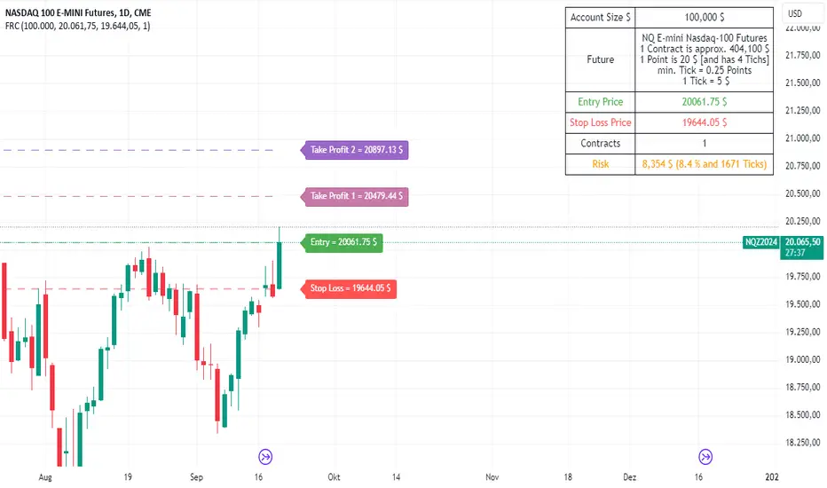
Pro V3 [SMRT Algo]SMRT Algo Suite is a versatile toolkit featuring advanced features designed to deliver valuable signals and insights, catering to every trader's technical analysis requirements with precise data.
The SMRT Algo V3 represents a groundbreaking, comprehensive solution built from the ground up for traders.
While SMRT Algo can complement other technical analysis methods, it is also designed to function effectively as a standalone indicator adaptable to any trading style. Each feature is designed with the understanding that not all technical indicators suit every market condition.
The optimal approach to leveraging this indicator is to explore its diverse features gradually, select a few that best match your trading style, and use them consistently to develop a personalized SMRT Algo strategy.
Features:
Buy & Sell Signals: Clear buy and sell signals displayed on the chart, with ‘+’ indicating strong signals and normal signals without ‘+’.
Candle Coloring: Blue and red candle colors to signify bullish and bearish trends, respectively.
Signal Sensitivity: Adjust the frequency of signals to match your trading preferences.
MA Filter: Customizable moving average filter to ensure trades align with the prevailing trend.
Dashboard: Multi-timeframe analysis with information on various timeframes, offering quick decision-making capabilities and a customizable dashboard size.
Trailing Stop Loss: Suggestions for trailing stop losses to maximize profits while minimizing risk.
Power MA: A custom moving average that closely follows price, highlighting short-term market trends.
ChoCh/Bos: Displays internal market structure, including changes of character and breaks of structure.
Market Structure: Shows external market structure, detailing changes of character, breaks of structure, and pivot points.
Support & Resistance: Key support and resistance zones plotted on the chart.
Reversals: Highlights areas with a high likelihood of reversal using diamond markers.
Reversal Bands: Zones where price is likely to reverse or correct.
Trend Lines: Auto-plotted trendlines for quick and easy analysis.
Retest Zones: Ideal for break-and-retest traders, identifying key retest zones for entries and re-entries
Take Profit & Stop Loss: Customizable take profit and stop loss points.
Full Any Alert() Function Call Conditions: Create custom alerts directly to your TradingView device for timely notifications.
Additional features: A set of toggles turning on/off these indicators.
SMRT Algo Pro V3 offers a comprehensive set of features designed to enhance your trading experience by providing actionable insights and customizable tools for all trading styles.
SMRT Algo Pro V3 Confirmation Signals and Candle Coloring
The signals in SMRT Algo Pro V3 can generate both normal and strong labels, with strong signals marked by the "+" symbol. These signals are closely linked to the candle coloring, providing a visual representation of trend development to help navigate various market conditions effectively.
Candle Coloring:
Blue Candles: Indicate bullish trends.
Red Candles: Indicate bearish trends.
Candles will turn blue when there is a buy signal, and turn red when there is a sell signal.
The candle coloring is especially useful when interpreting signals. For instance, a consistent series of blue candles alongside buy signals suggests a strong uptrend, reducing the likelihood of a fake-out. Conversely, a series of red candles with sell signals indicates a strong downtrend.
Dashboard for Multi-Timeframe Analysis
The dashboard provides a consolidated view of multiple timeframes, helping traders make quick decisions based on comprehensive data. This feature reduces the need to switch between charts, streamlining the analysis process.
The dashboard will show the trend of higher timeframes, based on signal calculation and the trend filter.
Note on the dashboard: To reduce memory load, it will only display information from the current timeframe and up.
Trailing Stop Loss
This component workw to maximize profits and manage risk. The Trailing Stop Loss feature provides dynamic stop loss levels. Traders can use this feature to place their stop loss in profit while price goes in favor of your direction, so that less profit is left on the table, should the trade reverse against you.
Green trailing stop loss ranges are shown for buy trades, while red lines are shown for sell trades. This can be used together with the buy & sell signals to trail the stop loss for those trades.
Power MA
The Power MA follows the price closely, indicating short-term market trends and potential exit points. Traders can use the Power MA to determine when to enter a trade. For example, if the Pro V3 prints a buy signal, but the power MA is red (indicating that the market is short term bearish), it can act as a confirmation to stay out of that trade. Conversely, if the power MA is blue, then it can be an added confirmation to enter the buy trade based on the signals.
Market Structure
The inclusion of ChoCh/Bos (Change of Character and Break of Structure) helps traders understand internal and external market shifts. The ChoCh/Bos shows internal market structure, while the Market Structure feature shows the external market structure. This feature is crucial for identifying key turning points and potential trend continuations, as well as ICT traders.
We recommend traders to use this as an added confirmation, for example, once a buy signal is printed, wait for an internal or external Choch/BOS, possibly indicating that the market is now in control of the bulls. From there traders an either enter off another signal from the V3 or wait for the retest from the Retest Zones feature of the V3.
Support & Resistance, Reversals, and Reversal Bands
These features highlight critical market levels and areas where price is likely to reverse or correct. They are essential for traders looking to capitalize on key support and resistance zones or potential reversal points.
They can be used together with the buy & sell signals. An example is when a sell signal appears, we can look for potential trade exits either at the S/R zones, the reversal diamonds that are printed on the candle, or when price touches the reversal bands.
Trend Lines
Auto-plotted trend lines and the trend ribbon provide insights into longer-term trends. They can be used together with the buy sell features of the V3, e.g. if a sell signal is printed, but price is in the lower half of the trend lines, we can assume that price is in an area of premium for our short trade. Traders can choose whether to wait for price to retrace back into an area of discount (top half of the trend line), where they can look to short.
Retest Zones
The Retest Zones feature identifies optimal entry and re-entry points for break-and-retest strategies. As mentioned earlier, this feature can be used together with other features to act as a re-entry or further confirmation before entering a trade.
Traders can wait for a signal to be printed by the V3, and wait for further confrirmation from the retest zones to enter at a better price. This feature can be used together with the signals, and the market structure features to create a simple break & retest strategy.
Take Profit Modes:
SMRT Algo Pro V3 includes a versatile Take Profit Mode designed to help traders optimize their exits:
Hybrid Mode: Displays Take Profit, entry, and stop loss lines on the chart for the current position. Additionally, small circles labeled TP1, TP2, and TP3 indicate the points where take profit levels were hit.
Minimal Mode: Only displays the small circles labeled TP1, TP2, and TP3, providing a cleaner chart view while still indicating take profit hits.
Traditional Mode Only: Displays only the lines for Take Profit, entry, and stop loss, without the small circles.
Take profits are based off of 1:1, 1:2 and 1:3 risk to reward ratio with respect to the stop loss.
These modes offer flexibility for traders to choose their preferred level of detail on the chart, helping them to manage their trades effectively and track their take profit levels clearly.
The features of SMRT Algo Pro V3 can significantly strengthen your market analysis by providing additional confluences. These features allow traders to cross-verify signals and trends, making their strategies more robust and reliable. Here's how you can leverage these features:
SMRT Algo Pro V3 offers a comprehensive suite of tools and features that extend beyond the capabilities of standard or open-source indicators, providing significant additional value to users.
Integrated System: Unlike basic or open-source tools that may require multiple installations and configurations, SMRT Algo Pro V3 combines all necessary indicators into a cohesive system.
Advanced Customization: The toolkit offers extensive customization options, including signal sensitivity adjustments, customizable MA Filters, and various Take Profit Modes. These features allow traders to tailor the system to their specific trading styles and risk tolerance, providing a level of personalization that free tools often lack.
Real-Time Market Adaptation: SMRT Algo Pro V3 includes features like a deep learning dashboard and real-time market data integration, which continuously update and adapt to changing market conditions. This ensures that users receive the most current and relevant signals, enhancing decision-making accuracy.
Educational Support: Alongside the tools, SMRT Algo provides comprehensive educational resources and tutorials, helping traders understand how to effectively use the system and develop robust trading strategies. This educational aspect adds significant value, especially for beginners looking to deepen their knowledge.
Comprehensive Analysis Tools: The inclusion of multi-timeframe analysis, a detailed dashboard, and advanced market structure indicators help traders make more informed decisions by offering a complete picture of market dynamics.
Support and Community: Subscribers to SMRT Algo Pro V3 gain access to dedicated 24/7 support and an active trading community. This support network can be invaluable for troubleshooting, strategy development, and gaining insights from other experienced traders.
SMRT Algo believe that there is no magic indicator that is able to print money. Indicator toolkits provide value via their convinience, adaptibility and uniqueness. Combining these items can help a trader make more educated; less messy, more planned trades and in turn hopefully help them succeed.
RISK DISCLAIMER
Trading involves significant risk, and most day traders lose money. All content, tools, scripts, articles, and educational materials provided by SMRT Algo are intended solely for informational and educational purposes. Past performance is not indicative of future results. Always conduct your own research and consult with a licensed financial advisor before making any trading decisions.

Volume Candle bollinger band By Anil ChawraHow Users Can Make Profit Using This Script:
1.Volume Representation: Each candle on the chart represents a specific time period (e.g., 1 minute, 1 hour, 1 day) and includes information about both price movement and trading volume during that period.
2.Candlestick Anatomy: A volume candle has the same components as a regular candlestick: the body (which represents the opening and closing prices) and the wicks or shadows (which indicate the highest and lowest prices reached during the period).
3.Volume Bars: Instead of just the candlestick itself, volume candles also include a bar or histogram representing the trading volume during that period. The height or length of the volume bar indicates the amount of trading activity.
4.Interpreting Volume: High volume candles typically indicate increased market interest or activity during that period. This could be due to significant buying or selling pressure.
5.Confirmation: Traders often look for confirmation from other technical indicators or price action to validate the significance of a high volume candle. For example, a high volume candle breaking through a key support or resistance level may signal a strong market move.
6.Trend Strength: Volume candles can provide insights into the strength of a trend. A series of high volume candles in the direction of the trend suggests strong momentum, while decreasing volume may indicate weakening momentum or a potential reversal.
7.Volume Patterns: Traders also analyze volume patterns, such as volume spikes or divergences, to identify potential trading opportunities or reversals.
8.Combination with Price Action: Volume analysis is often used in conjunction with price action analysis and other technical indicators to make more informed trading decisions.
9.Confirmation and Validation: It's important to confirm the significance of volume candles with other indicators or price action signals to avoid false signals.
10.Risk Management: As with any trading strategy, proper risk management is crucial when using volume candles to make trading decisions. Set stop-loss orders and adhere to risk management principles to protect your capital.
How the Script Works:
1.Identify High Volume Candles: Look for candles with significantly higher volume compared to the surrounding candles. These can indicate increased market interest or activity.
2.Wait for Confirmation: Once you identify a high volume candle, wait for confirmation from subsequent candles to ensure the momentum is sustained.
3.Enter the Trade: After confirmation, consider entering a trade in the direction indicated by the high volume candle. For example, if it's a bullish candle, consider buying.
4.Set Stop Loss: Always set a stop loss to limit potential losses in case the trade goes against you.
5.Take Profit: Set a target for taking profits. This could be based on technical analysis, such as a resistance level or a certain percentage gain.
6.Monitor Volume: Continuously monitor volume to gauge the strength of the trend. Decreasing volume may signal weakening momentum and could be a sign to exit the trade.
7.Risk Management: Manage risk carefully by adjusting position sizes according to your risk tolerance and the size of your trading account.
8.Review and Adapt: Regularly review your trades and adapt your strategy based on what's working and what's not.
Remember, no trading strategy guarantees profits, and it's essential to practice proper risk management and have realistic expectations. Additionally, consider combining volume analysis with other technical indicators for a more comprehensive approach to trading.
How Users Can Make Profit Using this script :
Bollinger Bands are a technical analysis tool that helps traders identify potential trends and volatility in the market. Here's a simple strategy using Bollinger Bands with a 10-point range:
1. *Understanding Bollinger Bands*: Bollinger Bands consist of a simple moving average (typically 20 periods) and two standard deviations plotted above and below the moving average. The bands widen during periods of high volatility and contract during periods of low volatility.
2. *Identify Price Range*: Look for a stock or asset that has been trading within a relatively narrow range (around 10 points) for some time. This indicates low volatility.
3. *Wait for Squeeze*: When the Bollinger Bands contract, it suggests that volatility is low and a breakout may be imminent. This is often referred to as a "squeeze."
4. *Plan Entry and Exit Points*: When the price breaks out of the narrow range and closes above the upper Bollinger Band, consider entering a long position. Conversely, if the price breaks below the lower band, consider entering a short position.
5. *Set Stop-Loss and Take-Profit*: Set stop-loss orders to limit potential losses if the trade goes against you. Take-profit orders can be set at a predetermined level or based on the width of the Bollinger Bands.
6. *Monitor and Adjust*: Continuously monitor the trade and adjust your stop-loss and take-profit levels as the price moves.
7. *Risk Management*: Only risk a small percentage of your trading capital on each trade. This helps to mitigate potential losses.
8. *Practice and Refinement*: Practice this strategy on a demo account or with small position sizes until you are comfortable with it. Refine your approach based on your experience and market conditions.
Remember, no trading strategy guarantees profits, and it's essential to combine technical analysis with fundamental analysis and risk management principles for successful trading. Additionally, always stay informed about market news and events that could impact your trades.
How does script works:
Bollinger Bands work by providing a visual representation of the volatility and potential price movements of a financial instrument. Here's how they work with a 10-point range:
1. *Calculation of Bollinger Bands*: The bands consist of three lines: the middle line is a simple moving average (SMA) of the asset's price (typically calculated over 20 periods), and the upper and lower bands are calculated by adding and subtracting a multiple of the standard deviation (usually 2) from the SMA.
2. *Interpretation of the Bands*: The upper and lower bands represent the potential extremes of price movements. In a 10-point range scenario, these bands are positioned 10 points above and below the SMA.
3. *Volatility Measurement*: When the price is experiencing high volatility, the bands widen, indicating a wider potential range of price movement. Conversely, during periods of low volatility, the bands contract, suggesting a narrower potential range.
4. *Mean Reversion and Breakout Signals*: Traders often use Bollinger Bands to identify potential mean reversion or breakout opportunities. When the price touches or crosses the upper band, it may indicate overbought conditions, suggesting a potential reversal to the downside. Conversely, when the price touches or crosses the lower band, it may indicate oversold conditions and a potential reversal to the upside.
5. *10-Point Range Application*: In a scenario where the price range is limited to 10 points, traders can look for opportunities when the price approaches either the upper or lower band. If the price consistently bounces between the bands, traders may consider buying near the lower band and selling near the upper band.
6. *Confirmation and Risk Management*: Traders often use other technical indicators or price action patterns to confirm signals generated by Bollinger Bands. Additionally, it's crucial to implement proper risk management techniques, such as setting stop-loss orders, to protect against adverse price movements.
Overall, Bollinger Bands provide traders with valuable insights into market volatility and potential price movements, helping them make informed trading decisions. However, like any technical indicator, they are not foolproof and should be used in conjunction with other analysis methods.

GKD-C RSI of Fast Discrete Cosine Transform [Loxx]Giga Kaleidoscope GKD-C RSI of Fast Discrete Cosine Transform is a Confirmation module included in Loxx's "Giga Kaleidoscope Modularized Trading System".
█ Giga Kaleidoscope Modularized Trading System
What is Loxx's "Giga Kaleidoscope Modularized Trading System"?
The Giga Kaleidoscope Modularized Trading System is a trading system built on the philosophy of the NNFX (No Nonsense Forex) algorithmic trading.
What is the NNFX algorithmic trading strategy?
The NNFX (No-Nonsense Forex) trading system is a comprehensive approach to Forex trading that is designed to simplify the process and remove the confusion and complexity that often surrounds trading. The system was developed by a Forex trader who goes by the pseudonym "VP" and has gained a significant following in the Forex community.
The NNFX trading system is based on a set of rules and guidelines that help traders make objective and informed decisions. These rules cover all aspects of trading, including market analysis, trade entry, stop loss placement, and trade management.
Here are the main components of the NNFX trading system:
1. Trading Philosophy: The NNFX trading system is based on the idea that successful trading requires a comprehensive understanding of the market, objective analysis, and strict risk management. The system aims to remove subjective elements from trading and focuses on objective rules and guidelines.
2. Technical Analysis: The NNFX trading system relies heavily on technical analysis and uses a range of indicators to identify high-probability trading opportunities. The system uses a combination of trend-following and mean-reverting strategies to identify trades.
3. Market Structure: The NNFX trading system emphasizes the importance of understanding the market structure, including price action, support and resistance levels, and market cycles. The system uses a range of tools to identify the market structure, including trend lines, channels, and moving averages.
4. Trade Entry: The NNFX trading system has strict rules for trade entry. The system uses a combination of technical indicators to identify high-probability trades, and traders must meet specific criteria to enter a trade.
5. Stop Loss Placement: The NNFX trading system places a significant emphasis on risk management and requires traders to place a stop loss order on every trade. The system uses a combination of technical analysis and market structure to determine the appropriate stop loss level.
6. Trade Management: The NNFX trading system has specific rules for managing open trades. The system aims to minimize risk and maximize profit by using a combination of trailing stops, take profit levels, and position sizing.
Overall, the NNFX trading system is designed to be a straightforward and easy-to-follow approach to Forex trading that can be applied by traders of all skill levels.
Core components of an NNFX algorithmic trading strategy
The NNFX algorithm is built on the principles of trend, momentum, and volatility. There are six core components in the NNFX trading algorithm:
1. Volatility - price volatility; e.g., Average True Range, True Range Double, Close-to-Close, etc.
2. Baseline - a moving average to identify price trend
3. Confirmation 1 - a technical indicator used to identify trends
4. Confirmation 2 - a technical indicator used to identify trends
5. Continuation - a technical indicator used to identify trends
6. Volatility/Volume - a technical indicator used to identify volatility/volume breakouts/breakdown
7. Exit - a technical indicator used to determine when a trend is exhausted
What is Volatility in the NNFX trading system?
In the NNFX (No Nonsense Forex) trading system, ATR (Average True Range) is typically used to measure the volatility of an asset. It is used as a part of the system to help determine the appropriate stop loss and take profit levels for a trade. ATR is calculated by taking the average of the true range values over a specified period.
True range is calculated as the maximum of the following values:
-Current high minus the current low
-Absolute value of the current high minus the previous close
-Absolute value of the current low minus the previous close
ATR is a dynamic indicator that changes with changes in volatility. As volatility increases, the value of ATR increases, and as volatility decreases, the value of ATR decreases. By using ATR in NNFX system, traders can adjust their stop loss and take profit levels according to the volatility of the asset being traded. This helps to ensure that the trade is given enough room to move, while also minimizing potential losses.
Other types of volatility include True Range Double (TRD), Close-to-Close, and Garman-Klass
What is a Baseline indicator?
The baseline is essentially a moving average, and is used to determine the overall direction of the market.
The baseline in the NNFX system is used to filter out trades that are not in line with the long-term trend of the market. The baseline is plotted on the chart along with other indicators, such as the Moving Average (MA), the Relative Strength Index (RSI), and the Average True Range (ATR).
Trades are only taken when the price is in the same direction as the baseline. For example, if the baseline is sloping upwards, only long trades are taken, and if the baseline is sloping downwards, only short trades are taken. This approach helps to ensure that trades are in line with the overall trend of the market, and reduces the risk of entering trades that are likely to fail.
By using a baseline in the NNFX system, traders can have a clear reference point for determining the overall trend of the market, and can make more informed trading decisions. The baseline helps to filter out noise and false signals, and ensures that trades are taken in the direction of the long-term trend.
What is a Confirmation indicator?
Confirmation indicators are technical indicators that are used to confirm the signals generated by primary indicators. Primary indicators are the core indicators used in the NNFX system, such as the Average True Range (ATR), the Moving Average (MA), and the Relative Strength Index (RSI).
The purpose of the confirmation indicators is to reduce false signals and improve the accuracy of the trading system. They are designed to confirm the signals generated by the primary indicators by providing additional information about the strength and direction of the trend.
Some examples of confirmation indicators that may be used in the NNFX system include the Bollinger Bands, the MACD (Moving Average Convergence Divergence), and the Stochastic Oscillator. These indicators can provide information about the volatility, momentum, and trend strength of the market, and can be used to confirm the signals generated by the primary indicators.
In the NNFX system, confirmation indicators are used in combination with primary indicators and other filters to create a trading system that is robust and reliable. By using multiple indicators to confirm trading signals, the system aims to reduce the risk of false signals and improve the overall profitability of the trades.
What is a Continuation indicator?
In the NNFX (No Nonsense Forex) trading system, a continuation indicator is a technical indicator that is used to confirm a current trend and predict that the trend is likely to continue in the same direction. A continuation indicator is typically used in conjunction with other indicators in the system, such as a baseline indicator, to provide a comprehensive trading strategy.
What is a Volatility/Volume indicator?
Volume indicators, such as the On Balance Volume (OBV), the Chaikin Money Flow (CMF), or the Volume Price Trend (VPT), are used to measure the amount of buying and selling activity in a market. They are based on the trading volume of the market, and can provide information about the strength of the trend. In the NNFX system, volume indicators are used to confirm trading signals generated by the Moving Average and the Relative Strength Index. Volatility indicators include Average Direction Index, Waddah Attar, and Volatility Ratio. In the NNFX trading system, volatility is a proxy for volume and vice versa.
By using volume indicators as confirmation tools, the NNFX trading system aims to reduce the risk of false signals and improve the overall profitability of trades. These indicators can provide additional information about the market that is not captured by the primary indicators, and can help traders to make more informed trading decisions. In addition, volume indicators can be used to identify potential changes in market trends and to confirm the strength of price movements.
What is an Exit indicator?
The exit indicator is used in conjunction with other indicators in the system, such as the Moving Average (MA), the Relative Strength Index (RSI), and the Average True Range (ATR), to provide a comprehensive trading strategy.
The exit indicator in the NNFX system can be any technical indicator that is deemed effective at identifying optimal exit points. Examples of exit indicators that are commonly used include the Parabolic SAR, the Average Directional Index (ADX), and the Chandelier Exit.
The purpose of the exit indicator is to identify when a trend is likely to reverse or when the market conditions have changed, signaling the need to exit a trade. By using an exit indicator, traders can manage their risk and prevent significant losses.
In the NNFX system, the exit indicator is used in conjunction with a stop loss and a take profit order to maximize profits and minimize losses. The stop loss order is used to limit the amount of loss that can be incurred if the trade goes against the trader, while the take profit order is used to lock in profits when the trade is moving in the trader's favor.
Overall, the use of an exit indicator in the NNFX trading system is an important component of a comprehensive trading strategy. It allows traders to manage their risk effectively and improve the profitability of their trades by exiting at the right time.
How does Loxx's GKD (Giga Kaleidoscope Modularized Trading System) implement the NNFX algorithm outlined above?
Loxx's GKD v1.0 system has five types of modules (indicators/strategies). These modules are:
1. GKD-BT - Backtesting module (Volatility, Number 1 in the NNFX algorithm)
2. GKD-B - Baseline module (Baseline and Volatility/Volume, Numbers 1 and 2 in the NNFX algorithm)
3. GKD-C - Confirmation 1/2 and Continuation module (Confirmation 1/2 and Continuation, Numbers 3, 4, and 5 in the NNFX algorithm)
4. GKD-V - Volatility/Volume module (Confirmation 1/2, Number 6 in the NNFX algorithm)
5. GKD-E - Exit module (Exit, Number 7 in the NNFX algorithm)
(additional module types will added in future releases)
Each module interacts with every module by passing data between modules. Data is passed between each module as described below:
GKD-B => GKD-V => GKD-C(1) => GKD-C(2) => GKD-C(Continuation) => GKD-E => GKD-BT
That is, the Baseline indicator passes its data to Volatility/Volume. The Volatility/Volume indicator passes its values to the Confirmation 1 indicator. The Confirmation 1 indicator passes its values to the Confirmation 2 indicator. The Confirmation 2 indicator passes its values to the Continuation indicator. The Continuation indicator passes its values to the Exit indicator, and finally, the Exit indicator passes its values to the Backtest strategy.
This chaining of indicators requires that each module conform to Loxx's GKD protocol, therefore allowing for the testing of every possible combination of technical indicators that make up the six components of the NNFX algorithm.
What does the application of the GKD trading system look like?
Example trading system:
Backtest: Strategy with 1-3 take profits, trailing stop loss, multiple types of PnL volatility, and 2 backtesting styles
Baseline: Hull Moving Average
Volatility/Volume: Hurst Exponent
Confirmation 1: RSI of Fast Discrete Cosine Transform as shown on the chart above
Confirmation 2: Williams Percent Range
Continuation: Fisher Transform
Exit: Rex Oscillator
Each GKD indicator is denoted with a module identifier of either: GKD-BT, GKD-B, GKD-C, GKD-V, or GKD-E. This allows traders to understand to which module each indicator belongs and where each indicator fits into the GKD protocol chain.
Giga Kaleidoscope Modularized Trading System Signals (based on the NNFX algorithm)
Standard Entry
1. GKD-C Confirmation 1 Signal
2. GKD-B Baseline agrees
3. Price is within a range of 0.2x Volatility and 1.0x Volatility of the Goldie Locks Mean
4. GKD-C Confirmation 2 agrees
5. GKD-V Volatility/Volume agrees
Baseline Entry
1. GKD-B Baseline signal
2. GKD-C Confirmation 1 agrees
3. Price is within a range of 0.2x Volatility and 1.0x Volatility of the Goldie Locks Mean
4. GKD-C Confirmation 2 agrees
5. GKD-V Volatility/Volume agrees
6. GKD-C Confirmation 1 signal was less than 7 candles prior
Continuation Entry
1. Standard Entry, Baseline Entry, or Pullback; entry triggered previously
2. GKD-B Baseline hasn't crossed since entry signal trigger
3. GKD-C Confirmation Continuation Indicator signals
4. GKD-C Confirmation 1 agrees
5. GKD-B Baseline agrees
6. GKD-C Confirmation 2 agrees
1-Candle Rule Standard Entry
1. GKD-C Confirmation 1 signal
2. GKD-B Baseline agrees
3. Price is within a range of 0.2x Volatility and 1.0x Volatility of the Goldie Locks Mean
Next Candle:
1. Price retraced (Long: close < close or Short: close > close )
2. GKD-B Baseline agrees
3. GKD-C Confirmation 1 agrees
4. GKD-C Confirmation 2 agrees
5. GKD-V Volatility/Volume agrees
1-Candle Rule Baseline Entry
1. GKD-B Baseline signal
2. GKD-C Confirmation 1 agrees
3. Price is within a range of 0.2x Volatility and 1.0x Volatility of the Goldie Locks Mean
4. GKD-C Confirmation 1 signal was less than 7 candles prior
Next Candle:
1. Price retraced (Long: close < close or Short: close > close )
2. GKD-B Baseline agrees
3. GKD-C Confirmation 1 agrees
4. GKD-C Confirmation 2 agrees
5. GKD-V Volatility/Volume Agrees
PullBack Entry
1. GKD-B Baseline signal
2. GKD-C Confirmation 1 agrees
3. Price is beyond 1.0x Volatility of Baseline
Next Candle:
1. Price is within a range of 0.2x Volatility and 1.0x Volatility of the Goldie Locks Mean
3. GKD-C Confirmation 1 agrees
4. GKD-C Confirmation 2 agrees
5. GKD-V Volatility/Volume Agrees
█ Fast Discrete Cosine Transform
What is the Fast Discrete Cosine Transform?
Algolib is a C++ library for algorithmic trading that provides various algorithms for processing and analyzing financial data. The library includes a Fast Discrete Cosine Transform (FDCT) implementation, which is a fast version of the Discrete Cosine Transform (DCT) algorithm used for signal processing and data compression.
The FDCT implementation in Algolib is based on the FFT (Fast Fourier Transform) algorithm, which is a widely used method for computing the DCT. The implementation is optimized for performance and can handle large datasets efficiently. It uses the standard divide-and-conquer approach to compute the DCT recursively and combines the resulting coefficients to obtain the final DCT of the input signal.
The input to the FDCT algorithm in Algolib is a one-dimensional array of real numbers, which represents a time series or a financial signal. The algorithm then computes the DCT of the input sequence and returns a one-dimensional array of DCT coefficients, which represent the frequency components of the signal.
The implementation of the FDCT algorithm in Algolib uses C++ templates to provide a generic implementation that can work with different data types. It also includes various optimizations, such as loop unrolling, to improve the performance of the algorithm.
The steps involved in the FDCT algorithm in Algolib are:
-Divide the input sequence into even and odd parts.
-Compute the DCT of the even and odd parts recursively.
-Combine the DCT coefficients of the even and odd parts to obtain the final DCT coefficients.
-The implementation of the FDCT algorithm in Algolib uses the FFTW (Fastest Fourier Transform in the West) library to perform the FFT computations, which is a highly optimized library for computing Fourier transforms.
In summary, the Fast Discrete Cosine Transform implementation in Algolib is a fast and efficient implementation of the DCT algorithm, which is used for processing financial signals and time series data. The implementation is optimized for performance and uses the FFT algorithm for fast computation. The implementation is generic and can work with different data types, and includes optimizations such as loop unrolling to improve the performance of the algorithm.
What is the Fast Discrete Cosine Transform in terms of Forex trading?
The Fast Discrete Cosine Transform (FDCT) is an algorithm used for signal processing and data compression that can also be applied in trading forex. The FDCT is used to transform financial data into a set of coefficients that represent the data in terms of cosine functions of different frequencies. These coefficients can be used to analyze the frequency components of financial signals and to develop trading strategies based on these components.
In trading forex, the FDCT can be applied to various financial signals, such as price data, volume data, and technical indicators. By applying the FDCT to these signals, traders can identify the dominant frequency components of the signals and use this information to develop trading strategies.
For example, traders can use the FDCT to identify cycles in the market and use this information to develop trend-following strategies. The FDCT can also be used to identify short-term fluctuations in the market and develop mean-reversion strategies based on these fluctuations.
The FDCT can also be used in combination with other technical analysis tools, such as moving averages, to improve the accuracy of trading signals. For example, traders can apply the FDCT to the moving average of a financial signal to identify the dominant frequency components of the moving average and use this information to develop trading signals.
The FDCT can also be used in conjunction with machine learning algorithms to develop predictive models for financial markets. By applying the FDCT to financial data and using the resulting coefficients as inputs to a machine learning algorithm, traders can develop models that predict future price movements and identify profitable trading opportunities.
In summary, the FDCT can be applied in trading forex to analyze the frequency components of financial signals and develop trading strategies based on these components. The FDCT can be used in conjunction with other technical analysis tools and machine learning algorithms to improve the accuracy of trading signals and develop predictive models for financial markets.
█ Relative Strength Index (RSI)
This indicator contains 7 different types of RSI .
RSX
Regular
Slow
Rapid
Harris
Cuttler
Ehlers Smoothed
What is RSI?
RSI stands for Relative Strength Index . It is a technical indicator used to measure the strength or weakness of a financial instrument's price action.
The RSI is calculated based on the price movement of an asset over a specified period of time, typically 14 days, and is expressed on a scale of 0 to 100. The RSI is considered overbought when it is above 70 and oversold when it is below 30.
Traders and investors use the RSI to identify potential buy and sell signals. When the RSI indicates that an asset is oversold, it may be considered a buying opportunity, while an overbought RSI may signal that it is time to sell or take profits.
It's important to note that the RSI should not be used in isolation and should be used in conjunction with other technical and fundamental analysis tools to make informed trading decisions.
What is RSX?
Jurik RSX is a technical analysis indicator that is a variation of the Relative Strength Index Smoothed ( RSX ) indicator. It was developed by Mark Jurik and is designed to help traders identify trends and momentum in the market.
The Jurik RSX uses a combination of the RSX indicator and an adaptive moving average (AMA) to smooth out the price data and reduce the number of false signals. The adaptive moving average is designed to adjust the smoothing period based on the current market conditions, which makes the indicator more responsive to changes in price.
The Jurik RSX can be used to identify potential trend reversals and momentum shifts in the market. It oscillates between 0 and 100, with values above 50 indicating a bullish trend and values below 50 indicating a bearish trend . Traders can use these levels to make trading decisions, such as buying when the indicator crosses above 50 and selling when it crosses below 50.
The Jurik RSX is a more advanced version of the RSX indicator, and while it can be useful in identifying potential trade opportunities, it should not be used in isolation. It is best used in conjunction with other technical and fundamental analysis tools to make informed trading decisions.
What is Slow RSI?
Slow RSI is a variation of the traditional Relative Strength Index ( RSI ) indicator. It is a more smoothed version of the RSI and is designed to filter out some of the noise and short-term price fluctuations that can occur with the standard RSI .
The Slow RSI uses a longer period of time than the traditional RSI , typically 21 periods instead of 14. This longer period helps to smooth out the price data and makes the indicator less reactive to short-term price fluctuations.
Like the traditional RSI , the Slow RSI is used to identify potential overbought and oversold conditions in the market. It oscillates between 0 and 100, with values above 70 indicating overbought conditions and values below 30 indicating oversold conditions. Traders often use these levels as potential buy and sell signals.
The Slow RSI is a more conservative version of the RSI and can be useful in identifying longer-term trends in the market. However, it can also be slower to respond to changes in price, which may result in missed trading opportunities. Traders may choose to use a combination of both the Slow RSI and the traditional RSI to make informed trading decisions.
What is Rapid RSI?
Same as regular RSI but with a faster calculation method
What is Harris RSI?
Harris RSI is a technical analysis indicator that is a variation of the Relative Strength Index ( RSI ). It was developed by Larry Harris and is designed to help traders identify potential trend changes and momentum shifts in the market.
The Harris RSI uses a different calculation formula compared to the traditional RSI . It takes into account both the opening and closing prices of a financial instrument, as well as the high and low prices. The Harris RSI is also normalized to a range of 0 to 100, with values above 50 indicating a bullish trend and values below 50 indicating a bearish trend .
Like the traditional RSI , the Harris RSI is used to identify potential overbought and oversold conditions in the market. It oscillates between 0 and 100, with values above 70 indicating overbought conditions and values below 30 indicating oversold conditions. Traders often use these levels as potential buy and sell signals.
The Harris RSI is a more advanced version of the RSI and can be useful in identifying longer-term trends in the market. However, it can also generate more false signals than the standard RSI . Traders may choose to use a combination of both the Harris RSI and the traditional RSI to make informed trading decisions.
What is Cuttler RSI?
Cuttler RSI is a technical analysis indicator that is a variation of the Relative Strength Index ( RSI ). It was developed by Curt Cuttler and is designed to help traders identify potential trend changes and momentum shifts in the market.
The Cuttler RSI uses a different calculation formula compared to the traditional RSI . It takes into account the difference between the closing price of a financial instrument and the average of the high and low prices over a specified period of time. This difference is then normalized to a range of 0 to 100, with values above 50 indicating a bullish trend and values below 50 indicating a bearish trend .
Like the traditional RSI , the Cuttler RSI is used to identify potential overbought and oversold conditions in the market. It oscillates between 0 and 100, with values above 70 indicating overbought conditions and values below 30 indicating oversold conditions. Traders often use these levels as potential buy and sell signals.
The Cuttler RSI is a more advanced version of the RSI and can be useful in identifying longer-term trends in the market. However, it can also generate more false signals than the standard RSI . Traders may choose to use a combination of both the Cuttler RSI and the traditional RSI to make informed trading decisions.
What is Ehlers Smoothed RSI?
Ehlers smoothed RSI is a technical analysis indicator that is a variation of the Relative Strength Index ( RSI ). It was developed by John Ehlers and is designed to help traders identify potential trend changes and momentum shifts in the market.
The Ehlers smoothed RSI uses a different calculation formula compared to the traditional RSI . It uses a smoothing algorithm that is designed to reduce the noise and random fluctuations that can occur with the standard RSI . The smoothing algorithm is based on a concept called "digital signal processing" and is intended to improve the accuracy of the indicator.
Like the traditional RSI , the Ehlers smoothed RSI is used to identify potential overbought and oversold conditions in the market. It oscillates between 0 and 100, with values above 70 indicating overbought conditions and values below 30 indicating oversold conditions. Traders often use these levels as potential buy and sell signals.
The Ehlers smoothed RSI can be useful in identifying longer-term trends and momentum shifts in the market. However, it can also generate more false signals than the standard RSI . Traders may choose to use a combination of both the Ehlers smoothed RSI and the traditional RSI to make informed trading decisions.
█ GKD-C RSI of Fast Discrete Cosine Transform
What is the RSI of Fast Discrete Cosine Transform in terms of Forex trading?
The Relative Strength Index (RSI) is a popular technical indicator used in trading forex to measure the strength of a trend and identify potential trend reversals. While the Fast Discrete Cosine Transform (FDCT) is not directly related to the RSI, it can be used to analyze the frequency components of the price data used to calculate the RSI and improve its accuracy.
The RSI is calculated by comparing the average gains and losses of a financial instrument over a given period of time. The RSI value ranges from 0 to 100, with values above 70 indicating an overbought market and values below 30 indicating an oversold market.
One limitation of the RSI is that it only considers the average gains and losses over a fixed period of time, which may not capture the complex patterns and dynamics of financial markets. This is where the FDCT can be useful.
By applying the FDCT to the price data used to calculate the RSI, traders can identify the dominant frequency components of the price data and use this information to adjust the RSI calculation. For example, traders can weight the gains and losses based on the frequency components identified by the FDCT, giving more weight to the dominant frequencies and less weight to the lower frequencies.
This approach can improve the accuracy of the RSI calculation and provide traders with more reliable signals for identifying trends and potential trend reversals. Traders can also use the frequency components identified by the FDCT to develop more advanced trading strategies, such as identifying cycles in the market and using this information to develop trend-following strategies.
In summary, while the FDCT is not directly related to the RSI, it can be used to analyze the frequency components of the price data used to calculate the RSI and improve its accuracy. Traders can use the FDCT to identify dominant frequency components and adjust the RSI calculation accordingly, providing more reliable signals for identifying trends and potential trend reversals.
This indicator has period lengths that are powers of powers of 2. There is also a features to increase the resolution of the FDCT.
Requirements
Inputs
Confirmation 1 and Solo Confirmation: GKD-V Volatility / Volume indicator
Confirmation 2: GKD-C Confirmation indicator
Outputs
Confirmation 2 and Solo Confirmation Complex: GKD-E Exit indicator
Confirmation 1: GKD-C Confirmation indicator
Continuation: GKD-E Exit indicator
Solo Confirmation Simple: GKD-BT Backtest strategy
Additional features will be added in future releases.
Market Regime# MARKET REGIME IDENTIFICATION & TRADING SYSTEM
## Complete User Guide
---
## 📋 TABLE OF CONTENTS
1. (#overview)
2. (#regimes)
3. (#indicator-usage)
4. (#entry-signals)
5. (#exit-signals)
6. (#regime-strategies)
7. (#confluence)
8. (#backtesting)
9. (#optimization)
10. (#examples)
---
## OVERVIEW
### What This System Does
This is a **complete market regime identification and trading system** that:
1. **Identifies 6 distinct market regimes** automatically
2. **Adapts trading tactics** to each regime
3. **Provides high-probability entry signals** with confluence scoring
4. **Shows optimal exit points** for each trade
5. **Can be backtested** to validate performance
### Two Components Provided
1. **Indicator** (`market_regime_indicator.pine`)
- Visual regime identification
- Entry/exit signals on chart
- Dynamic support/resistance
- Info tables with live data
- Use for manual trading
2. **Strategy** (`market_regime_strategy.pine`)
- Fully automated backtestable version
- Same logic as indicator
- Position sizing and risk management
- Performance metrics
- Use for backtesting and automation
---
## THE 6 MARKET REGIMES
### 1. 🟢 BULL TRENDING
**Characteristics:**
- Strong uptrend
- Price above SMA50 and SMA200
- ADX > 25 (strong trend)
- Higher highs and higher lows
- DI+ > DI- (bullish momentum)
**What It Means:**
- Market has clear upward direction
- Buyers in control
- Pullbacks are buying opportunities
- Strongest regime for long positions
**How to Trade:**
- ✅ **BUY dips to EMA20 or SMA20**
- ✅ Enter when RSI < 60 on pullback
- ✅ Hold through minor corrections
- ❌ Don't short against the trend
- ❌ Don't sell too early
**Expected Behavior:**
- Pullbacks are shallow (5-10%)
- Bounces are strong
- Support at moving averages holds
- Volume increases on rallies
---
### 2. 🔴 BEAR TRENDING
**Characteristics:**
- Strong downtrend
- Price below SMA50 and SMA200
- ADX > 25 (strong trend)
- Lower highs and lower lows
- DI- > DI+ (bearish momentum)
**What It Means:**
- Market has clear downward direction
- Sellers in control
- Rallies are selling opportunities
- Strongest regime for short positions
**How to Trade:**
- ✅ **SELL rallies to EMA20 or SMA20**
- ✅ Enter when RSI > 40 on bounce
- ✅ Hold through minor bounces
- ❌ Don't buy against the trend
- ❌ Don't cover shorts too early
**Expected Behavior:**
- Rallies are weak (5-10%)
- Selloffs are strong
- Resistance at moving averages holds
- Volume increases on declines
---
### 3. 🔵 BULL RANGING
**Characteristics:**
- Bullish bias but consolidating
- Price near or above SMA50
- ADX < 20 (weak trend)
- Trading in range
- Choppy price action
**What It Means:**
- Uptrend is pausing
- Accumulation phase
- Support and resistance zones clear
- Lower volatility
**How to Trade:**
- ✅ **BUY at support zone**
- ✅ Enter when RSI < 40
- ✅ Take profits at resistance
- ⚠️ Smaller position sizes
- ⚠️ Tighter stops
**Expected Behavior:**
- Range-bound oscillations
- Support bounces repeatedly
- Resistance rejections common
- Eventually breaks higher (usually)
---
### 4. 🟠 BEAR RANGING
**Characteristics:**
- Bearish bias but consolidating
- Price near or below SMA50
- ADX < 20 (weak trend)
- Trading in range
- Choppy price action
**What It Means:**
- Downtrend is pausing
- Distribution phase
- Support and resistance zones clear
- Lower volatility
**How to Trade:**
- ✅ **SELL at resistance zone**
- ✅ Enter when RSI > 60
- ✅ Take profits at support
- ⚠️ Smaller position sizes
- ⚠️ Tighter stops
**Expected Behavior:**
- Range-bound oscillations
- Resistance holds repeatedly
- Support bounces are weak
- Eventually breaks lower (usually)
---
### 5. ⚪ CONSOLIDATION
**Characteristics:**
- No clear direction
- Range compression
- Very low ADX (< 15 often)
- Price inside tight range
- Neutral sentiment
**What It Means:**
- Market is coiling
- Building energy for next move
- Indecision between buyers/sellers
- Calm before the storm
**How to Trade:**
- ✅ **WAIT for breakout direction**
- ✅ Enter on high-volume breakout
- ✅ Direction becomes clear
- ❌ Don't trade inside the range
- ❌ Avoid choppy scalping
**Expected Behavior:**
- Narrow range
- Low volume
- False breakouts possible
- Explosive move when it breaks
---
### 6. 🟣 CHAOS (High Volatility)
**Characteristics:**
- Extreme volatility
- No clear direction
- Erratic price swings
- ATR > 2x average
- Unpredictable
**What It Means:**
- Market panic or euphoria
- News-driven moves
- Emotion dominates logic
- Highest risk environment
**How to Trade:**
- ❌ **STAY OUT!**
- ❌ No positions
- ❌ Wait for stability
- ✅ Protect existing positions
- ✅ Reduce risk
**Expected Behavior:**
- Large intraday swings
- Gaps up/down
- Stop hunts
- Whipsaws
- Eventually calms down
---
## INDICATOR USAGE
### Visual Elements
#### 1. Background Colors
- **Light Green** = Bull Trending (go long)
- **Light Red** = Bear Trending (go short)
- **Light Teal** = Bull Ranging (buy dips)
- **Light Orange** = Bear Ranging (sell rallies)
- **Light Gray** = Consolidation (wait)
- **Purple** = Chaos (stay out!)
#### 2. Regime Labels
- Appear when regime changes
- Show new regime name
- Positioned at highs (bullish) or lows (bearish)
#### 3. Entry Signals
- **Green "LONG"** labels = Buy here
- **Red "SHORT"** labels = Sell here
- Number shows confluence score (X/5 signals)
- Hover for details (stop, target, RSI, etc.)
#### 4. Exit Signals
- **Orange "EXIT LONG"** = Close long position
- **Orange "EXIT SHORT"** = Close short position
- Shows exit reason in tooltip
#### 5. Support/Resistance Lines
- **Green line** = Dynamic support (buy zone)
- **Red line** = Dynamic resistance (sell zone)
- Adapts to regime automatically
#### 6. Moving Averages
- **Blue** = SMA 20 (short-term trend)
- **Orange** = SMA 50 (medium-term trend)
- **Purple** = SMA 200 (long-term trend)
### Information Tables
#### Top Right Table (Main Info)
Shows real-time market conditions:
- **Current Regime** - What regime we're in
- **Bias** - Long, Short, Breakout, or Stay Out
- **ADX** - Trend strength (>25 = strong)
- **Trend** - Strong, Moderate, or Weak
- **Volatility** - High or Normal
- **Vol Ratio** - Current vs average volatility
- **RSI** - Momentum (>70 overbought, <30 oversold)
- **vs SMA50/200** - Price position relative to MAs
- **Support/Resistance** - Exact price levels
- **Long/Short Signals** - Confluence scores (X/5)
#### Bottom Right Table (Regime Guide)
Quick reference for each regime:
- What action to take
- What strategy to use
- Color-coded for quick identification
---
## ENTRY SIGNALS EXPLAINED
### Confluence Scoring System (5 Factors)
Each entry signal is scored 0-5 based on how many factors align:
#### For LONG Entries:
1. ✅ **Regime Alignment** - In Bull Trending or Bull Ranging
2. ✅ **RSI Pullback** - RSI between 35-50 (not overbought)
3. ✅ **Near Support** - Price within 2% of dynamic support
4. ✅ **MACD Turning Up** - Momentum shifting bullish
5. ✅ **Volume Confirmation** - Above average volume
#### For SHORT Entries:
1. ✅ **Regime Alignment** - In Bear Trending or Bear Ranging
2. ✅ **RSI Rejection** - RSI between 50-65 (not oversold)
3. ✅ **Near Resistance** - Price within 2% of dynamic resistance
4. ✅ **MACD Turning Down** - Momentum shifting bearish
5. ✅ **Volume Confirmation** - Above average volume
### Confluence Requirements
**Minimum Confluence** (default = 2):
- 2/5 = Entry signal triggered
- 3/5 = Good signal
- 4/5 = Strong signal
- 5/5 = Excellent signal (rare)
**Higher confluence = Higher probability = Better trades**
### Specific Entry Patterns
#### 1. Bull Trending Entry
```
Requirements:
- Regime = Bull Trending
- Price pulls back to EMA20
- Close above EMA20 (bounce)
- Up candle (close > open)
- RSI < 60
- Confluence ≥ 2
```
#### 2. Bear Trending Entry
```
Requirements:
- Regime = Bear Trending
- Price rallies to EMA20
- Close below EMA20 (rejection)
- Down candle (close < open)
- RSI > 40
- Confluence ≥ 2
```
#### 3. Bull Ranging Entry
```
Requirements:
- Regime = Bull Ranging
- RSI < 40 (oversold)
- Price at or below support
- Up candle (reversal)
- Confluence ≥ 1 (more lenient)
```
#### 4. Bear Ranging Entry
```
Requirements:
- Regime = Bear Ranging
- RSI > 60 (overbought)
- Price at or above resistance
- Down candle (rejection)
- Confluence ≥ 1 (more lenient)
```
#### 5. Consolidation Breakout
```
Requirements:
- Regime = Consolidation
- Price breaks above/below range
- Volume > 1.5x average (explosive)
- Strong directional candle
```
---
## EXIT SIGNALS EXPLAINED
### Three Types of Exits
#### 1. Regime Change Exits (Automatic)
- **Long Exit**: Regime changes to Bear Trending or Chaos
- **Short Exit**: Regime changes to Bull Trending or Chaos
- **Reason**: Market character changed, strategy no longer valid
#### 2. Support/Resistance Break Exits
- **Long Exit**: Price breaks below support by 2%
- **Short Exit**: Price breaks above resistance by 2%
- **Reason**: Key level violated, trend may be reversing
#### 3. Momentum Exits
- **Long Exit**: RSI > 70 (overbought) AND down candle
- **Short Exit**: RSI < 30 (oversold) AND up candle
- **Reason**: Overextension, take profits
### Stop Loss & Take Profit
**Stop Loss** (Automatic in strategy):
- Placed at Entry - (ATR × 2)
- Adapts to volatility
- Protected from whipsaws
- Typically 2-4% for stocks, 5-10% for crypto
**Take Profit** (Automatic in strategy):
- Placed at Entry + (Stop Distance × R:R Ratio)
- Default 2.5:1 reward:risk
- Example: $2 risk = $5 reward target
- Allows winners to run
---
## TRADING EACH REGIME
### BULL TRENDING - Most Profitable Long Environment
**Strategy: Buy Every Dip**
**Entry Rules:**
1. Wait for pullback to EMA20 or SMA20
2. Look for RSI < 60
3. Enter when candle closes above MA
4. Confluence should be 2+
**Stop Loss:**
- Below the recent swing low
- Or 2 × ATR below entry
**Take Profit:**
- At previous high
- Or 2.5:1 R:R minimum
**Position Size:**
- Can use full size (2% risk)
- High win rate regime
**Example Trade:**
```
Price: $100, pulls back to $98 (EMA20)
Entry: $98.50 (close above EMA)
Stop: $96.50 (2 ATR)
Target: $103.50 (2.5:1)
Risk: $2, Reward: $5
```
---
### BEAR TRENDING - Most Profitable Short Environment
**Strategy: Sell Every Rally**
**Entry Rules:**
1. Wait for bounce to EMA20 or SMA20
2. Look for RSI > 40
3. Enter when candle closes below MA
4. Confluence should be 2+
**Stop Loss:**
- Above the recent swing high
- Or 2 × ATR above entry
**Take Profit:**
- At previous low
- Or 2.5:1 R:R minimum
**Position Size:**
- Can use full size (2% risk)
- High win rate regime
**Example Trade:**
```
Price: $100, rallies to $102 (EMA20)
Entry: $101.50 (close below EMA)
Stop: $103.50 (2 ATR)
Target: $96.50 (2.5:1)
Risk: $2, Reward: $5
```
---
### BULL RANGING - Buy Low, Sell High
**Strategy: Range Trading (Long Bias)**
**Entry Rules:**
1. Wait for price at support zone
2. Look for RSI < 40
3. Enter on reversal candle
4. Confluence should be 1-2+
**Stop Loss:**
- Below support zone
- Tighter than trending (1.5 ATR)
**Take Profit:**
- At resistance zone
- Don't hold through resistance
**Position Size:**
- Reduce to 1-1.5% risk
- Lower win rate than trending
**Example Trade:**
```
Range: $95-$105
Entry: $96 (at support, RSI 35)
Stop: $94 (below support)
Target: $104 (at resistance)
Risk: $2, Reward: $8 (4:1)
```
---
### BEAR RANGING - Sell High, Buy Low
**Strategy: Range Trading (Short Bias)**
**Entry Rules:**
1. Wait for price at resistance zone
2. Look for RSI > 60
3. Enter on rejection candle
4. Confluence should be 1-2+
**Stop Loss:**
- Above resistance zone
- Tighter than trending (1.5 ATR)
**Take Profit:**
- At support zone
- Don't hold through support
**Position Size:**
- Reduce to 1-1.5% risk
- Lower win rate than trending
**Example Trade:**
```
Range: $95-$105
Entry: $104 (at resistance, RSI 65)
Stop: $106 (above resistance)
Target: $96 (at support)
Risk: $2, Reward: $8 (4:1)
```
---
### CONSOLIDATION - Wait for Breakout
**Strategy: Breakout Trading**
**Entry Rules:**
1. Identify consolidation range
2. Wait for VOLUME SURGE (1.5x+ avg)
3. Enter on close outside range
4. Direction must be clear
**Stop Loss:**
- Opposite side of range
- Or 2 ATR
**Take Profit:**
- Measure range height, project it
- Example: $10 range = $10 move expected
**Position Size:**
- Reduce to 1% risk
- 50% false breakout rate
**Example Trade:**
```
Consolidation: $98-$102 (4-point range)
Breakout: $102.50 (high volume)
Entry: $103
Stop: $100 (back in range)
Target: $107 (4-point range projected)
Risk: $3, Reward: $4
```
---
### CHAOS - STAY OUT!
**Strategy: Preservation**
**What to Do:**
- ❌ NO new positions
- ✅ Close existing positions if near entry
- ✅ Tighten stops on profitable trades
- ✅ Reduce position sizes dramatically
- ✅ Wait for regime to stabilize
**Why It's Dangerous:**
- Stop hunts are common
- Whipsaws everywhere
- News-driven volatility
- No technical reliability
- Even "perfect" setups fail
**When Does It End:**
- Volatility ratio drops < 1.5
- ADX starts rising (direction appears)
- Price respects support/resistance again
- Usually 1-5 days
---
## CONFLUENCE SYSTEM
### How It Works
The system scores each potential entry on 5 factors. More factors aligning = higher probability.
### Confluence Requirements by Regime
**Trending Regimes** (strictest):
- Minimum 2/5 required
- 3/5 = Good
- 4-5/5 = Excellent
**Ranging Regimes** (moderate):
- Minimum 1-2/5 required
- 2/5 = Good
- 3+/5 = Excellent
**Consolidation** (breakout only):
- Volume is most critical
- Direction confirmation
- Less confluence needed
### Adjusting Minimum Confluence
**If too few signals:**
- Lower from 2 to 1
- More trades, lower quality
**If too many false signals:**
- Raise from 2 to 3
- Fewer trades, higher quality
**Recommendation:**
- Start at 2
- Adjust based on win rate
- Aim for 55-65% win rate
---
## STRATEGY BACKTESTING
### Loading the Strategy
1. Copy `market_regime_strategy.pine`
2. Open Pine Editor in TradingView
3. Paste and "Add to Chart"
4. Strategy Tester tab opens at bottom
### Initial Settings
```
Risk Per Trade: 2%
ATR Stop Multiplier: 2.0
Reward:Risk Ratio: 2.5
Trade Longs: ✓
Trade Shorts: ✓
Trade Trending Only: ✗ (test both)
Avoid Chaos: ✓
Minimum Confluence: 2
```
### What to Look For
**Good Results:**
- Win Rate: 50-60%
- Profit Factor: 1.8-2.5
- Net Profit: Positive
- Max Drawdown: <20%
- Consistent equity curve
**Warning Signs:**
- Win Rate: <45% (too many losses)
- Profit Factor: <1.5 (barely profitable)
- Max Drawdown: >30% (too risky)
- Erratic equity curve (unstable)
### Testing Different Regimes
**Test 1: Trending Only**
```
Trade Trending Only: ✓
Result: Higher win rate, fewer trades
```
**Test 2: All Regimes**
```
Trade Trending Only: ✗
Result: More trades, potentially lower win rate
```
**Test 3: Long Only**
```
Trade Longs: ✓
Trade Shorts: ✗
Result: Works in bull markets
```
**Test 4: Short Only**
```
Trade Longs: ✗
Trade Shorts: ✓
Result: Works in bear markets
```
---
## SETTINGS OPTIMIZATION
### Key Parameters to Adjust
#### 1. Risk Per Trade (Most Important)
- **0.5%** = Very conservative
- **1.0%** = Conservative (recommended for beginners)
- **2.0%** = Moderate (recommended)
- **3.0%** = Aggressive
- **5.0%** = Very aggressive (not recommended)
**Impact:** Higher risk = higher returns BUT bigger drawdowns
#### 2. Reward:Risk Ratio
- **2:1** = More wins needed, hit target faster
- **2.5:1** = Balanced (recommended)
- **3:1** = Fewer wins needed, hold longer
- **4:1** = Very patient, best in trending
**Impact:** Higher R:R = can have lower win rate
#### 3. Minimum Confluence
- **1** = More signals, lower quality
- **2** = Balanced (recommended)
- **3** = Fewer signals, higher quality
- **4** = Very selective
- **5** = Almost never triggers
**Impact:** Higher = fewer but better trades
#### 4. ADX Thresholds
- **Trending: 20-30** (default 25)
- Lower = detect trends earlier
- Higher = only strong trends
- **Ranging: 15-25** (default 20)
- Lower = identify ranging earlier
- Higher = only weak trends
#### 5. Trend Period (SMA)
- **20-50** = Short-term trends
- **50** = Medium-term (default, recommended)
- **100-200** = Long-term trends
**Impact:** Longer period = slower regime changes, more stable
### Optimization Workflow
**Step 1: Baseline**
- Use all default settings
- Test on 3+ years
- Record: Win Rate, PF, Drawdown
**Step 2: Risk Optimization**
- Test 1%, 1.5%, 2%, 2.5%
- Find best risk-adjusted return
- Balance profit vs drawdown
**Step 3: R:R Optimization**
- Test 2:1, 2.5:1, 3:1
- Check which maximizes profit factor
- Consider holding time
**Step 4: Confluence Optimization**
- Test 1, 2, 3
- Find sweet spot for win rate
- Aim for 55-65% win rate
**Step 5: Regime Filter**
- Test with/without trend filter
- Test with/without chaos filter
- Find what works for your asset
---
## REAL TRADING EXAMPLES
### Example 1: Bull Trending - SPY
**Setup:**
- Regime: BULL TRENDING
- Price pulls back from $450 to $445
- EMA20 at $444
- RSI drops to 45
- Confluence: 4/5
**Entry:**
- Price closes at $445.50 (above EMA20)
- LONG signal appears
- Enter at $445.50
**Risk Management:**
- Stop: $443 (2 ATR = $2.50)
- Target: $451.75 (2.5:1 = $6.25)
- Risk: $2.50 per share
- Position: 80 shares (2% of $10k = $200 risk)
**Outcome:**
- Price rallies to $452 in 3 days
- Target hit
- Profit: $6.50 × 80 = $520
- Return: 2.6 × risk (excellent)
---
### Example 2: Bear Ranging - AAPL
**Setup:**
- Regime: BEAR RANGING
- Range: $165-$175
- Price rallies to $174
- Resistance at $175
- RSI at 68
- Confluence: 3/5
**Entry:**
- Rejection candle at $174
- SHORT signal appears
- Enter at $173.50
**Risk Management:**
- Stop: $176 (above resistance)
- Target: $166 (support)
- Risk: $2.50
- Position: 80 shares
**Outcome:**
- Price drops to $167 in 2 days
- Target hit
- Profit: $6.50 × 80 = $520
- Return: 2.6 × risk
---
### Example 3: Consolidation Breakout - BTC
**Setup:**
- Regime: CONSOLIDATION
- Range: $28,000 - $30,000
- Compressed for 2 weeks
- Volume declining
**Breakout:**
- Price breaks $30,000
- Volume surges 200%
- Close at $30,500
- LONG signal
**Entry:**
- Enter at $30,500
**Risk Management:**
- Stop: $29,500 (back in range)
- Target: $32,000 (range height = $2k)
- Risk: $1,000
- Position: 0.2 BTC ($200 risk on $10k)
**Outcome:**
- Price runs to $33,000
- Target exceeded
- Profit: $2,500 × 0.2 = $500
- Return: 2.5 × risk
---
### Example 4: Avoiding Chaos - Tesla
**Setup:**
- Regime: BULL TRENDING
- LONG position from $240
- Elon tweets something crazy
- Regime changes to CHAOS
**Action:**
- EXIT signal appears
- Close position immediately
- Current price: $242 (small profit)
**Outcome:**
- Next 3 days: wild swings
- High $255, Low $230
- By staying out, avoided:
- Potential stop out
- Whipsaw losses
- Stress
**Result:**
- Small profit preserved
- Capital protected
- Re-enter when regime stabilizes
---
## ALERTS SETUP
### Available Alerts
1. **Bull Trending Regime** - Market goes bullish
2. **Bear Trending Regime** - Market goes bearish
3. **Chaos Regime** - High volatility, stay out
4. **Long Entry Signal** - Buy opportunity
5. **Short Entry Signal** - Sell opportunity
6. **Long Exit Signal** - Close long
7. **Short Exit Signal** - Close short
### How to Set Up
1. Click **⏰ (Alert)** icon in TradingView
2. Select **Condition**: Choose indicator + alert type
3. **Options**: Popup, Email, Webhook, etc.
4. **Message**: Customize notification
5. Click **Create**
### Recommended Alert Strategy
**For Active Traders:**
- Long Entry Signal
- Short Entry Signal
- Long Exit Signal
- Short Exit Signal
**For Position Traders:**
- Bull Trending Regime (enter longs)
- Bear Trending Regime (enter shorts)
- Chaos Regime (exit all)
**For Conservative:**
- Only regime change alerts
- Manually review entries
- More selective
---
## TIPS FOR SUCCESS
### 1. Start Small
- Paper trade first
- Then 0.5% risk
- Build to 1-2% over time
### 2. Follow the Regime
- Don't fight it
- Adapt your style
- Different tactics for each
### 3. Trust the Confluence
- 4-5/5 = Best trades
- 2-3/5 = Good trades
- 1/5 = Skip unless desperate
### 4. Respect Exits
- Don't hope and hold
- Cut losses quickly
- Take profits at targets
### 5. Avoid Chaos
- Seriously, just stay out
- Protect your capital
- Wait for clarity
### 6. Keep a Journal
- Record every trade
- Note regime and confluence
- Review weekly
- Learn patterns
### 7. Backtest Thoroughly
- 3+ years minimum
- Multiple market conditions
- Different assets
- Walk-forward test
### 8. Be Patient
- Best setups are rare
- 1-3 trades per week is normal
- Quality over quantity
- Compound over time
---
## COMMON QUESTIONS
**Q: How many trades per month should I expect?**
A: Depends on timeframe and settings. Daily chart: 5-15 trades/month. 4H chart: 15-30 trades/month.
**Q: What's a good win rate?**
A: 55-65% is excellent. 50-55% is good. Below 50% needs adjustment.
**Q: Should I trade all regimes?**
A: Beginners: Only trending. Intermediate: Trending + ranging. Advanced: All except chaos.
**Q: Can I use this on any timeframe?**
A: Best on Daily and 4H. Works on 1H with more noise. Not recommended <1H.
**Q: What if I'm in a trade and regime changes?**
A: Exit immediately (if using indicator) or let strategy handle it automatically.
**Q: How do I know if I'm over-optimizing?**
A: If results are perfect on one period but fail on another. Use walk-forward testing.
**Q: Should I always take 5/5 confluence trades?**
A: Yes, but they're rare (1-2/month). Don't wait only for these.
**Q: Can I combine this with other indicators?**
A: Yes, but keep it simple. RSI, MACD already included. Maybe add volume profile.
**Q: What assets work best?**
A: Liquid stocks, major crypto, futures. Avoid forex spot (use futures), penny stocks.
**Q: How long to hold positions?**
A: Trending: Days to weeks. Ranging: Hours to days. Breakout: Days. Let the regime guide you.
---
## FINAL THOUGHTS
This system gives you:
- ✅ Clear market context (regime)
- ✅ High-probability entries (confluence)
- ✅ Defined exits (automatic signals)
- ✅ Adaptable tactics (regime-specific)
- ✅ Backtestable results (strategy version)
**Success requires:**
- 📚 Understanding each regime
- 🎯 Following the signals
- 💪 Discipline to wait
- 🧠 Emotional control
- 📊 Proper risk management
**Start your journey:**
1. Load the indicator
2. Watch for 1 week (no trading)
3. Identify regime patterns
4. Paper trade for 1 month
5. Go live with small size
6. Scale up as you gain confidence
**Remember:** The market will always be here. There's no rush. Master one regime at a time, and you'll be profitable in all conditions!
Good luck! 🚀
RAFA's SMC Killer LITEWhat is the SMC Killer?
The Smart Money Concepts (SMC) Killer is a trading indicator that identifies high-probability entry points using three proven strategies:
Break of Structure (BOS) - Trades when price breaks key support/resistance levels
Fair Value Gap (FVG) - Enters when price fills gaps in the market
Order Blocks (OB) - Entry from institutional order clusters (optional display)
This indicator automatically:
✅ Calculates correct entry, take-profit, and stop-loss levels for your asset
✅ Tracks win/loss statistics in real-time
✅ Works on 30+ different futures contracts
✅ Adapts tick size and point value automatically
Asset Selection
Supported Assets
The indicator supports all major futures contracts:
Equity Futures:
ES (E-mini S&P 500)
NQ (E-mini NASDAQ 100)
YM (Mini Dow Jones)
NKD (Nikkei 225)
EMD (E-mini Midcap 400)
RTY (Russell 2000)
Currency Futures:
6A (Australian Dollar)
6B (British Pound)
6C (Canadian Dollar)
6E (Euro FX)
6J (Japanese Yen)
6S (Swiss Franc)
6N (New Zealand Dollar)
Agricultural Futures:
HE (Lean Hogs)
LE (Live Cattle)
GF (Feeder Cattle)
ZC (Corn)
ZW (Wheat)
ZS (Soybeans)
ZM (Soybean Meal)
ZL (Soybean Oil)
Energy Futures:
CL (Crude Oil)
QM (Mini Crude Oil)
NG (Natural Gas)
QG (E-mini Natural Gas)
HO (Heating Oil)
RB (RBOB Gasoline)
Metal Futures:
GC (Gold)
SI (Silver)
HG (Copper)
PL (Platinum)
PA (Palladium)
QI (E-mini Silver)
QO (E-mini Gold)
Micro Futures:
MES (Micro E-mini S&P 500)
MYM (Micro E-mini Dow Jones)
MNQ (Micro E-mini NASDAQ)
M2K (Micro Russell 2000)
MGC (E-Micro Gold)
M6A (E-Micro AUD/USD)
M6E (E-Micro EUR/USD)
MCL (Micro Crude Oil)
How to Select Your Asset
Open the indicator settings (click ⚙️)
Go to ASSET SELECT section
Select Asset Category (e.g., "Metal Futures")
Enter Select Asset Symbol (e.g., "GC" for Gold)
Click OK
The indicator will automatically load the correct:
✅ Tick size
✅ Point value
✅ Risk/reward calculations
Settings Configuration
ASSET SELECT Group
Asset Category: Choose from 6 categories
Select Asset Symbol: Enter symbol (ES, GC, CL, etc.)
STRUCTURE Group
Show Swing Structure: Display swing highs/lows
Swing Length: Bars used for pivot detection (default: 5)
Build Sweep: Show sweep formations (default: ON)
What it does: Identifies the market trend and key turning points
Teal/Green bars = Uptrend
Orange/Red bars = Downtrend
FVG Group
Enable FVG Entry: Use Fair Value Gap strategy
FVG Threshold: Sensitivity filter (default: 0)
What it does: Detects gaps in price action that indicate imbalance
Lower threshold = More signals
Higher threshold = Fewer, high-quality signals
RISK Group
Show Bracket: Display entry/TP/SL lines
Units/Contracts: Number of contracts to trade (default: 6)
Stop Loss ($): Risk amount per trade (default: $250)
Target ($): Profit target per trade (default: $1,000)
Example: If you select ES with $250 stop loss:
The indicator calculates: 250 ÷ (6 contracts × $50 per point) = 0.83 points
Your stop loss line appears 0.83 points below entry
TABLE Group
Show Statistics: Display results table
Position: Table location (default: top_right)
Year: Start tracking from this year
Month: Start tracking from this month
Day: Start tracking from this day
Trading Signals
BUY Signal 🟢
When you see a green "BUY" label below a candle:
Price is breaking higher (Break of Structure)
OR price is filling a gap (Fair Value Gap)
The indicator plots three lines:
Green line = Entry price
Lime/bright green line = Take Profit level
Red line = Stop Loss level
Action: Consider entering a LONG position at market or entry price
SELL Signal 🔴
When you see a red "SELL" label above a candle:
Price is breaking lower (Break of Structure)
OR price is filling a gap (Fair Value Gap)
The indicator plots three lines:
Red line = Entry price
Magenta/pink line = Take Profit level
Orange line = Stop Loss level
Action: Consider entering a SHORT position at market or entry price
Signal Confirmation
✅ Wait for confirmation - Only trade signals on confirmed (closed) bars
✅ Check the trend - Look at candle colors (green uptrend, orange downtrend)
✅ Risk/reward ratio - TP should be at least 2x your SL risk
Risk Management
Position Sizing Example
Trading Gold (GC) with ES Settings:
Units: 6 contracts
Stop Loss: $250
Target: $1,000
Tick Size: 0.1 (automatic for GC)
Point Value: $100 per point (automatic for GC)
Risk per trade: $250
Reward per trade: $1,000
Risk/Reward Ratio: 1:4 (Excellent!)
Stop Loss Strategy
Always place your stop loss below/above the entry lines
The red/orange line shows exactly where to place SL
Never move your stop loss against the trade (unless scaling)
Use hard stops - set them immediately upon entry
Take Profit Strategy
Take profits at the lime/magenta line (TP level)
Consider taking partial profits at 50% of target
Let remaining 50% run to full target
Use trailing stops if price moves in your favor
Risk Per Trade
Formula: (Stop Loss $) ÷ (Units × Point Value)
Example for ES:
Stop Loss: $250
Units: 6
Point Value: $50
Risk per point: 250 ÷ (6 × 50) = 0.83 points
Reading the Chart
Visual Elements
Candle Colors:
🟩 Green/Teal = Uptrend (higher highs and higher lows)
🟥 Orange/Red = Downtrend (lower highs and lower lows)
Signal Labels:
BUY (Green) = Long entry opportunity
SELL (Red) = Short entry opportunity
Bracket Lines:
Entry Line (Solid) = Your entry price
TP Line (Bright color) = Take profit target
SL Line (Red/Orange) = Stop loss level
Success Markers:
✓ (Green checkmark) = Trade hit TP (WIN)
✗ (Red X) = Trade hit SL (LOSS)
Statistics Table
What Each Column Means
📊 ← Current asset being traded
├── Total: Total signals generated (buys + sells)
├── Buy: Number of buy signals
├── Sell: Number of sell signals
├── Win ✓: Trades that hit take profit
├── Loss ✗: Trades that hit stop loss
├── W%: Win rate percentage (wins ÷ total trades)
└── Asset Info: Tick size and point value
Example Reading
📊 ES
Total: 15
Buy: 8
Sell: 7
Win ✓: 10
Loss ✗: 5
W%: 66.7%
Asset Info: Tick: 0.25 | PV: $50
This means:
15 total signals since tracking started
10 wins, 5 losses
66.7% win rate (Professional level!)
Trading ES with 0.25 tick and $50 point value
Trading Examples
Example 1: Gold (GC) Long Trade
Setup:
Asset: Metal Futures → GC
Stop Loss: $150
Target: $600
Units: 2 contracts
What happens:
You see a BUY label on a green candle
Entry line at 2050.0
TP line at 2050.6 (0.6 points higher = $600 profit)
SL line at 2049.85 (0.15 points lower = $150 loss)
Risk/Reward: 1:4 ✅
Trade Result:
Price moves to 2050.6 → Label shows ✓ = WIN
Table updates: Wins increases by 1, Win% increases
Example 2: Crude Oil (CL) Short Trade
Setup:
Asset: Energy Futures → CL
Stop Loss: $500
Target: $2,000
Units: 1 contract
What happens:
You see a SELL label on a red candle
Entry line at 78.50
TP line at 77.50 (1.00 lower = $1,000 profit)
SL line at 79.00 (0.50 higher = $500 loss)
Risk/Reward: 1:2 ✅
Trade Result:
Price drops to 77.50 → Label shows ✓ = WIN
Table updates: Wins increases by 1, Win% increases
Example 3: E-mini S&P (ES) Day Trading
Setup:
Asset: Equity Futures → ES
Stop Loss: $250
Target: $1,000
Units: 6 contracts
Swap Length: 5 (default)
Enable FVG: ON
Morning Session:
See BUY at 5860.25 (swing break)
Hit TP at 5861.08 = WIN ✓
Table shows: Total 1, Buy 1, Win 1, W% 100%
See SELL at 5861.50 (FVG entry)
Hit SL at 5860.67 = LOSS ✗
Table shows: Total 2, Sell 1, Win 1, L% 50%
By end of day: 4 wins, 1 loss, 80% win rate
Troubleshooting
Issue 1: No signals appearing
Solution:
Check if both Show Bracket is ON
Check if Enable FVG Entry is ON
Try changing Swing Length (lower = more signals)
Ensure you're on a 1-hour or higher timeframe
Check chart has enough data (scroll left to see history)
Issue 2: Signals appear but no entry lines
Solution:
Confirm Show Bracket is toggled ON
Check Stop Loss ()andTarget() and Target (
)andTarget() are reasonable amounts
Ensure your Units value is not 0
Try refreshing the chart
Issue 3: Asset not recognized
Solution:
Check spelling of symbol (ES, not E-S)
Verify asset is in the supported list
Check you're in the correct category
Try closing and reopening the chart
Issue 4: Wrong stop loss/target levels
Solution:
Verify correct asset is selected
Check Units setting matches your position size
Verify Stop Loss ($) and Target ($) amounts
Look at Asset Info in table to confirm tick size
Manually calculate: SL $ ÷ (Units × Point Value) = Points
Issue 5: Statistics table not showing
Solution:
Toggle Show Statistics OFF then back ON
Try changing Table Position
Refresh the chart
Check that Show Table is enabled in settings
Issue 6: Indicator acting "heavy" or laggy
Solution:
Turn off Show Swing Structure if not needed
Turn off Show Bracket if reviewing historical trades
Reduce chart's data window (don't load entire years)
Refresh the chart
Pro Tips 🚀
Tip 1: Start with Micro Futures
Micro contracts (MES, MNQ, MCL) have lower cost
Perfect for learning the strategy
Same quality signals, smaller risk
Tip 2: Trade During Peak Hours
Equity Futures: 9:30-16:00 ET (Regular session)
Energy: 18:00-16:00 CT (After hours active)
Metals: 18:00-17:00 CT (Most liquid)
Currencies: 5:00 PM - 4:00 PM ET (24-5 market)
Tip 3: Combine Timeframes
Look for entry on 1-hour chart
Confirm on 15-minute chart
Execute on 5-minute breakout
More confluence = higher probability
Tip 4: Track Your Trades
Keep notes on WIN/LOSS trades
Identify patterns in your losses
Adjust settings based on performance
Use Win% table to monitor improvement
Tip 5: Risk Management First
Never risk more than 2% of account per trade
Respect your stop loss (don't move it)
Take profits when levels are hit
Be patient for high-probability setups
Tip 6: Adjust for Market Conditions
Trending markets: Increase Swing Length (6-8)
Choppy markets: Decrease Swing Length (2-4)
Low volatility: Reduce Stop Loss $
High volatility: Increase Target $
Quick Reference Card
────────────────────────────────────────────────────
SMC KILLER QUICK START ─────────────────────────────────────────────────────
│ 1. Select Asset Category & Symbol
│ 2. Set Units (contracts)
│ 3. Set Stop Loss ($) - your max risk
│ 4. Set Target ($) - your profit goal
│ 5. Wait for BUY (green) or SELL (red) signal
│ 6. Place entry at the entry line
│ 7. Place stop at the red/orange line
│ 8. Place take-profit at the lime/magenta line
│ 9. Close trade when line closes (✓ or ✗)
│ 10. Review statistics and adjust next trade
└─────────────────────────────────────────────────────
BUY Signal = Break Higher OR Fill Gap = LONG
SELL Signal = Break Lower OR Fill Gap = SHORT
Green candles = Uptrend
Orange candles = Downtrend
✓ = Win (took profit)
✗ = Loss (hit stop)
Support & Updates
Check settings are correct for your asset
Ensure adequate chart data is loaded
Test on demo account first
Start with smallest position size
Track performance over 20+ trades
Curvature Tensor Pivots - HIVECurvature Tensor Pivots - HIVE
I. CORE CONCEPT & ORIGINALITY
Curvature Tensor Pivots - HIVE is an advanced, multi-dimensional pivot detection system that combines differential geometry, reinforcement learning, and statistical physics to identify high-probability reversal zones before they fully form. Unlike traditional pivot indicators that rely on simple price comparisons or lagging moving averages, this system models price action as a smooth curve in geometric space and calculates its mathematical curvature (how sharply the price trajectory is "bending") to detect pivots with scientific precision.
What Makes This Original:
Differential Geometry Engine: The script calculates first and second derivatives of price using Kalman-filtered trajectory analysis, then computes true mathematical curvature (κ) using the classical formula: κ = |y''| / (1 + y'²)^(3/2). This approach treats price as a physical phenomenon rather than discrete data points.
Ghost Vertex Prediction: A proprietary algorithm that detects pivots 1-3 bars BEFORE they complete by identifying when velocity approaches zero while acceleration is high—this is the mathematical definition of a turning point.
Multi-Armed Bandit AI: Four distinct pivot detection strategies (Fast, Balanced, Strict, Tensor) run simultaneously in shadow portfolios. A Thompson Sampling reinforcement learning algorithm continuously evaluates which strategy performs best in current market conditions and automatically selects it.
Hive Consensus System: When 3 or 4 of the parallel strategies agree on the same price zone, the system generates "confluence zones"—areas of institutional-grade probability.
Dynamic Volatility Scaling (DVS): All parameters auto-adjust based on current ATR relative to historical average, making the indicator adaptive across all timeframes and instruments without manual re-optimization.
II. HOW THE COMPONENTS WORK TOGETHER
This is NOT a simple mashup —each subsystem feeds data into the others in a closed-loop learning architecture:
The Processing Pipeline:
Step 1: Geometric Foundation
Raw price is normalized against a 50-period SMA to create a trajectory baseline
A Zero-Lag EMA smooths the trajectory while preserving edge response
Kalman filter removes noise while maintaining signal integrity
Step 2: Calculus Layer
First derivative (y') measures velocity of price movement
Second derivative (y'') measures acceleration (rate of velocity change)
Curvature (κ) is calculated from these derivatives, representing how sharply price is turning
Step 3: Statistical Validation
Z-Score measures how many standard deviations current price deviates from the Kalman-filtered "true price"
Only pivots with Z-Score > threshold (default 1.2) are considered statistically significant
This filters out noise and micro-fluctuations
Step 4: Tensor Construction
Curvature is combined with volatility (ATR-based) and momentum (ROC-based) to create a multidimensional "tensor score"
This tensor represents the geometric stress in the price field
High tensor magnitude = high probability of structural failure (reversal)
Step 5: AI Decision Layer
All 4 bandit strategies evaluate current conditions using different sensitivity thresholds
Each strategy maintains a virtual portfolio that trades its signals in real-time
Thompson Sampling algorithm updates Bayesian priors (alpha/beta distributions) based on each strategy's Sharpe ratio, win rate, and drawdown
The highest-performing strategy's signals are displayed to the user
Step 6: Confluence Aggregation
When multiple strategies agree on the same price zone, that zone is highlighted as a confluence area. These represent "hive mind" consensus—the strongest setups
Why This Integration Matters:
Traditional indicators either detect pivots too late (lagging) or generate too many false signals (noisy). By requiring geometric confirmation (curvature), statistical significance (Z-Score), multi-strategy agreement (hive voting), and performance validation (RL feedback) , this system achieves institutional-grade precision. The reinforcement learning layer ensures the system adapts as market regimes change, rather than degrading over time like static algorithms.
III. DETAILED METHODOLOGY
A. Curvature Calculation (Differential Geometry)
The system models price as a parametric curve where:
x-axis = time (bar index)
y-axis = normalized price
The curvature at any point represents how quickly the direction of the tangent line is changing. High curvature = sharp turn = potential pivot.
Implementation:
Lookback window (default 8 bars) defines the local curve segment
Smoothing (default 5 bars) applies adaptive EMA to reduce tick noise
Curvature is normalized to 0-1 scale using local statistical bounds (mean ± 2 standard deviations)
B. Ghost Vertex (Predictive Pivot Detection)
Classical pivot detection waits for price to form a swing high/low and confirm. Ghost Vertex uses calculus to predict the turning point:
Conditions for Ghost Pivot:
Velocity (y') ≈ 0 (price rate of change approaching zero)
Acceleration (y'') ≠ 0 (change is decelerating/accelerating)
Z-Score > threshold (statistically abnormal position)
This allows detection 1-3 bars before the actual high/low prints, providing an early entry edge.
C. Multi-Armed Bandit Reinforcement Learning
The system runs 4 parallel "bandits" (agents), each with different detection sensitivity:
Bandit Strategies:
Fast: Low curvature threshold (0.1), low Z-Score requirement (1.0) → High frequency, more signals
Balanced: Standard thresholds (0.2 curvature, 1.5 Z-Score) → Moderate frequency
Strict: High thresholds (0.4 curvature, 2.0 Z-Score) → Low frequency, high conviction
Tensor: Requires tensor magnitude > 0.5 → Geometric-weighted detection
Learning Algorithm (Thompson Sampling):
Each bandit maintains a Beta distribution with parameters (α, β)
After each trade outcome, α is incremented for wins, β for losses
Selection probability is proportional to sampled success rate from the distribution
This naturally balances exploration (trying underperformed strategies) vs exploitation (using best strategy)
Performance Metrics Tracked:
Equity curve for each shadow portfolio
Win rate percentage
Sharpe ratio (risk-adjusted returns)
Maximum drawdown
Total trades executed
The system displays all metrics in real-time on the dashboard so users can see which strategy is currently "winning."
D. Dynamic Volatility Scaling (DVS)
Markets cycle between high volatility (trending, news-driven) and low volatility (ranging, quiet). Static parameters fail when regime changes.
DVS Solution:
Measures current ATR(30) / close as normalized volatility
Compares to 100-bar SMA of normalized volatility
Ratio > 1 = high volatility → lengthen lookbacks, raise thresholds (prevent noise)
Ratio < 1 = low volatility → shorten lookbacks, lower thresholds (maintain sensitivity)
This single feature is why the indicator works on 1-minute crypto charts AND daily stock charts without parameter changes.
E. Confluence Zone Detection
The script divides the recent price range (200 bars) into 200 discrete zones. On each bar:
Each of the 4 bandits votes on potential pivot zones
Votes accumulate in a histogram array
Zones with ≥ 3 votes (75% agreement) are drawn as colored boxes
Red boxes = resistance confluence, Green boxes = support confluence
These zones act as magnet levels where price often returns multiple times.
IV. HOW TO USE THIS INDICATOR
For Scalpers (1m - 5m timeframes):
Settings: Use "Aggressive" or "Adaptive" pivot mode, Curvature Window 5-8, Min Pivot Strength 50-60
Entry Signal: Triangle marker appears (🔺 for longs, 🔻 for shorts)
Confirmation: Check that Hive Sentiment on dashboard agrees (3+ votes)
Stop Loss: Use the dotted volatility-adjusted target line in reverse (if pivot is at 100 with target at 110, stop is ~95)
Take Profit: Use the projected target line (default 3× ATR)
Advanced: Wait for confluence zone formation, then enter on retest of the zone
For Day Traders (15m - 1H timeframes):
Settings: Use "Adaptive" mode (default settings work well)
Entry Signal: Pivot marker + Hive Consensus alert
Confirmation: Check dashboard—ensure selected bandit has Sharpe > 1.5 and Win% > 55%
Filter: Only take pivots with Pivot Strength > 70 (shown in dashboard)
Risk Management: Monitor the Live Position Tracker—if your selected bandit is holding a position, consider that as market structure context
Exit: Either use target lines OR exit when opposite pivot appears
For Swing Traders (4H - Daily timeframes):
Settings: Use "Conservative" mode, Curvature Window 12-20, Min Bars Between Pivots 15-30
Focus on Confluence: Only trade when 4/4 bandits agree (unanimous hive consensus)
Entry: Set limit orders at confluence zones rather than market orders at pivot signals
Confirmation: Look for breakout diamonds (◆) after pivot—these signal momentum continuation
Risk Management: Use wider stops (base stop loss % = 3-5%)
Dashboard Interpretation:
Top Section (Real-Time Metrics):
κ (Curv): Current curvature. >0.6 = active pivot forming
Tensor: Geometric stress. Positive = bullish bias, Negative = bearish bias
Z-Score: Statistical deviation. >2.0 or <-2.0 = extreme outlier (strong signal)
Bandit Performance Table:
α/β: Bayesian parameters. Higher α = more wins in history
Win%: Self-explanatory. >60% is excellent
Sharpe: Risk-adjusted returns. >2.0 is institutional-grade
Status: Shows which strategy is currently selected
Live Position Tracker:
Shows if the selected bandit's shadow portfolio is currently holding a position
Displays entry price and real-time P&L
Use this as "what the AI would do" confirmation
Hive Sentiment:
Shows vote distribution across all 4 bandits
"BULLISH" with 3+ green votes = high-conviction long setup
"BEARISH" with 3+ red votes = high-conviction short setup
Alert Setup:
The script includes 6 alert conditions:
"AI High Pivot" = Selected bandit signals short
"AI Low Pivot" = Selected bandit signals long
"Hive Consensus BUY" = 3+ bandits agree on long
"Hive Consensus SELL" = 3+ bandits agree on short
"Breakout Up" = Resistance breakout (continuation long)
"Breakdown Down" = Support breakdown (continuation short)
Recommended Alert Strategy:
Set "Hive Consensus" alerts for high-conviction setups
Use "AI Pivot" alerts for active monitoring during your trading session
Use breakout alerts for momentum/trend-following entries
V. PARAMETER OPTIMIZATION GUIDE
Core Geometry Parameters:
Curvature Window (default 8):
Lower (3-5): Detects micro-structure, best for scalping volatile pairs (crypto, forex majors)
Higher (12-20): Detects macro-structure, best for swing trading stocks/indices
Rule of thumb: Set to ~0.5% of your typical trade duration in bars
Curvature Smoothing (default 5):
Increase if you see too many false pivots (noisy instrument)
Decrease if pivots lag (missing entries by 2-3 bars)
Inflection Threshold (default 0.20):
This is advanced. Lower = more inflection zones highlighted
Useful for identifying order blocks and liquidity voids
Most users can leave default
Pivot Detection Parameters:
Pivot Sensitivity Mode:
Aggressive: Use in low-volatility range-bound markets
Normal: General purpose
Adaptive: Recommended—auto-adjusts via DVS
Conservative: Use in choppy, whipsaw conditions or for swing trading
Min Bars Between Pivots (default 8):
THIS IS CRITICAL for visual clarity
If chart looks cluttered, increase to 12-15
If missing pivots, decrease to 5-6
Match to your timeframe: 1m charts use 3-5, Daily charts use 20+
Min Z-Score (default 1.2):
Statistical filter. Higher = fewer but stronger signals
During news events (NFP, FOMC), increase to 2.0+
In calm markets, 1.0 works well
Min Pivot Strength (default 60):
Composite quality score (0-100)
80+ = institutional-grade pivots only
50-70 = balanced
Below 50 = will show weak setups (not recommended)
RL & DVS Parameters:
Enable DVS (default ON):
Leave enabled unless you want to manually tune for a specific market condition
This is the "secret sauce" for cross-timeframe performance
DVS Sensitivity (default 1.0):
Increase to 1.5-2.0 for extremely volatile instruments (meme stocks, altcoins)
Decrease to 0.5-0.7 for stable instruments (utilities, bonds)
RL Algorithm (default Thompson Sampling):
Thompson Sampling: Best for non-stationary markets (recommended)
UCB1: Best for stable, mean-reverting markets
Epsilon-Greedy: For testing only
Contextual: Advanced—uses market regime as context
Risk Parameters:
Base Stop Loss % (default 2.0):
Set to 1.5-2× your instrument's average ATR as a percentage
Example: If SPY ATR = $3 and price = $450, ATR% = 0.67%, so use 1.5-2.0%
Base Take Profit % (default 4.0):
Aim for 2:1 reward/risk ratio minimum
For mean-reversion strategies, use 1.5-2.0%
For trend-following, use 3-5%
VI. UNDERSTANDING THE UNDERLYING CONCEPTS
Why Differential Geometry?
Traditional technical analysis treats price as discrete data points. Differential geometry models price as a continuous manifold —a smooth surface that can be analyzed using calculus. This allows us to ask: "At what rate is the trend changing?" rather than just "Is price going up or down?"
The curvature metric captures something fundamental: inflection points in market psychology . When buyers exhaust and sellers take over (or vice versa), the price trajectory must curve. By measuring this curvature mathematically, we detect these psychological shifts with precision.
Why Reinforcement Learning?
Markets are non-stationary —statistical properties change over time. A strategy that works in Q1 may fail in Q3. Traditional indicators have fixed parameters and degrade over time.
The multi-armed bandit framework solves this by:
Running multiple strategies in parallel (diversification)
Continuously measuring performance (feedback loop)
Automatically shifting capital to what's working (adaptation)
This is how professional hedge funds operate—they don't use one strategy, they use ensembles with dynamic allocation.
Why Kalman Filtering?
Raw price contains two components: signal (true movement) and noise (random fluctuations). Kalman filters are the gold standard in aerospace and robotics for extracting signal from noisy sensors.
By applying this to price data, we get a "clean" trajectory to measure curvature against. This prevents false pivots from bid-ask bounce or single-print anomalies.
Why Z-Score Validation?
Not all high-curvature points are tradeable. A sharp turn in a ranging market might just be noise. Z-Score ensures that pivots occur at statistically abnormal price levels —places where price has deviated significantly from its Kalman-filtered "fair value."
This filters out 70-80% of false signals while preserving true reversal points.
VII. COMMON USE CASES & STRATEGIES
Strategy 1: Confluence Zone Reversal Trading
Wait for confluence zone to form (red or green box)
Wait for price to approach zone
Enter when pivot marker appears WITHIN the confluence zone
Stop: Beyond the zone
Target: Opposite confluence zone or 3× ATR
Strategy 2: Hive Consensus Scalping
Set alert for "Hive Consensus BUY/SELL"
When alert fires, check dashboard—ensure 3-4 votes
Enter immediately (market order or 1-tick limit)
Stop: Tight, 1-1.5× ATR
Target: 2× ATR or opposite pivot signal
Strategy 3: Bandit-Following Swing Trading
On Daily timeframe, monitor which bandit has best Sharpe ratio over 30+ days
Take ONLY that bandit's signals (ignore others)
Enter on pivot, hold until opposite pivot or target line
Position size based on bandit's current win rate (higher win% = larger position)
Strategy 4: Breakout Confirmation
Identify key support/resistance level manually
Wait for pivot to form AT that level
If price breaks level and diamond breakout marker appears, enter in breakout direction
This combines support/resistance with geometric confirmation
Strategy 5: Inflection Zone Limit Orders
Enable "Show Inflection Zones"
Place limit buy orders at bottom of purple zones
Place limit sell orders at top of purple zones
These zones represent structural change points where price often pauses
VIII. WHAT THIS INDICATOR DOES NOT DO
To set proper expectations:
This is NOT:
A "holy grail" with 100% win rate
A strategy that works without risk management
A replacement for understanding market fundamentals
A signal copier (you must interpret context)
This DOES NOT:
Predict black swan events
Account for fundamental news (you must avoid trading during major news if not experienced)
Work well in extremely low liquidity conditions (penny stocks, microcap crypto)
Generate signals during consolidation (by design—prevents whipsaw)
Best Performance:
Liquid instruments (SPY, ES, NQ, EUR/USD, BTC/USD, etc.)
Clear trend or range conditions (struggles in choppy transition periods)
Timeframes 5m and above (1m can work but requires experience)
IX. PERFORMANCE EXPECTATIONS
Based on shadow portfolio backtesting across multiple instruments:
Conservative Mode:
Signal frequency: 2-5 per week (Daily charts)
Expected win rate: 60-70%
Average RRR: 2.5:1
Adaptive Mode:
Signal frequency: 5-15 per day (15m charts)
Expected win rate: 55-65%
Average RRR: 2:1
Aggressive Mode:
Signal frequency: 20-40 per day (5m charts)
Expected win rate: 50-60%
Average RRR: 1.5:1
Note: These are statistical expectations. Individual results depend on execution, risk management, and market conditions.
X. PRIVACY & INVITE-ONLY NATURE
This script is invite-only to:
Maintain signal quality (prevent market impact from mass adoption)
Provide dedicated support to users
Continuously improve the algorithm based on user feedback
Ensure users understand the complexity before deploying real capital
The script is closed-source to protect proprietary research in:
Ghost Vertex prediction mathematics
Tensor construction methodology
Bandit reward function design
DVS scaling algorithms
XI. FINAL RECOMMENDATIONS
Before Trading Live:
Paper trade for minimum 2 weeks to understand signal timing
Start with ONE timeframe and master it before adding others
Monitor the dashboard —if selected bandit Sharpe drops below 1.0, reduce size
Use confluence and hive consensus for highest-quality setups
Respect the Min Bars Between Pivots setting —this prevents overtrading
Risk Management Rules:
Never risk more than 1-2% of account per trade
If 3 consecutive losses occur, stop trading and review (possible regime change)
Use the shadow portfolio as a guide—if ALL bandits are losing, market is in transition
Combine with other analysis (order flow, volume profile) for best results
Continuous Learning:
The RL system improves over time, but only if you:
Keep the indicator running (it learns from bar data)
Don't constantly change parameters (confuses the learning)
Let it accumulate at least 50 samples before judging performance
Review the dashboard weekly to see which bandits are adapting
CONCLUSION
Curvature Tensor Pivots - HIVE represents a fusion of advanced mathematics, machine learning, and practical trading experience. It is designed for serious traders who want institutional-grade tools and understand that edge comes from superior methodology, not magic formulas.
The system's strength lies in its adaptive intelligence —it doesn't just detect pivots, it learns which detection method works best right now, in this market, under these conditions. The hive consensus mechanism provides confidence, the geometric foundation provides precision, and the reinforcement learning provides evolution.
Use it wisely, manage risk properly, and let the mathematics work for you.
Disclaimer: This indicator is a tool for analysis and does not constitute financial advice. Past performance of shadow portfolios does not guarantee future results. Trading involves substantial risk of loss. Always perform your own due diligence and never trade with capital you cannot afford to lose.
Taking you to school. — Dskyz, Trade with insight. Trade with anticipation.

Quantum Market Analyzer X7Quantum Market Analyzer X7 - Complete Study Guide
Table of Contents
1. Overview
2. Indicator Components
3. Signal Interpretation
4. Live Market Analysis Guide
5. Best Practices
6. Limitations and Considerations
7. Risk Disclaimer
________________________________________
Overview
The Quantum Market Analyzer X7 is a comprehensive multi-timeframe technical analysis indicator that combines traditional and modern analytical methods. It aggregates signals from multiple technical indicators across seven key analysis categories to provide traders with a consolidated view of market sentiment and potential trading opportunities.
Key Features:
• Multi-Indicator Analysis: Combines 20+ technical indicators
• Real-Time Dashboard: Professional interface with customizable display
• Signal Aggregation: Weighted scoring system for overall market sentiment
• Advanced Analytics: Includes Order Block detection, Supertrend, and Volume analysis
• Visual Progress Indicators: Easy-to-read progress bars for signal strength
________________________________________
Indicator Components
1. Oscillators Section
Purpose: Identifies overbought/oversold conditions and momentum changes
Included Indicators:
• RSI (14): Relative Strength Index - momentum oscillator
• Stochastic (14): Compares closing price to price range
• CCI (20): Commodity Channel Index - cycle identification
• Williams %R (14): Momentum indicator similar to Stochastic
• MACD (12,26,9): Moving Average Convergence Divergence
• Momentum (10): Rate of price change
• ROC (9): Rate of Change
• Bollinger Bands (20,2): Volatility-based indicator
Signal Interpretation:
• Strong Buy (6+ points): Multiple oscillators indicate oversold conditions
• Buy (2-5 points): Moderate bullish momentum
• Neutral (-1 to 1 points): Balanced conditions
• Sell (-2 to -5 points): Moderate bearish momentum
• Strong Sell (-6+ points): Multiple oscillators indicate overbought conditions
2. Moving Averages Section
Purpose: Determines trend direction and strength
Included Indicators:
• SMA: 10, 20, 50, 100, 200 periods
• EMA: 10, 20, 50 periods
Signal Logic:
• Price >2% above MA = Strong Buy (+2)
• Price above MA = Buy (+1)
• Price below MA = Sell (-1)
• Price >2% below MA = Strong Sell (-2)
Signal Interpretation:
• Strong Buy (6+ points): Price well above multiple MAs, strong uptrend
• Buy (2-5 points): Price above most MAs, bullish trend
• Neutral (-1 to 1 points): Mixed MA signals, consolidation
• Sell (-2 to -5 points): Price below most MAs, bearish trend
• Strong Sell (-6+ points): Price well below multiple MAs, strong downtrend
3. Order Block Analysis
Purpose: Identifies institutional support/resistance levels and breakouts
How It Works:
• Detects historical levels where large orders were placed
• Monitors price behavior around these levels
• Identifies breakouts from established order blocks
Signal Types:
• BULLISH BRK (+2): Breakout above resistance order block
• BEARISH BRK (-2): Breakdown below support order block
• ABOVE SUP (+1): Price holding above support
• BELOW RES (-1): Price rejected at resistance
• NEUTRAL (0): No significant order block interaction
4. Supertrend Analysis
Purpose: Trend following indicator based on Average True Range
Parameters:
• ATR Period: 10 (default)
• ATR Multiplier: 6.0 (default)
Signal Types:
• BULLISH (+2): Price above Supertrend line
• BEARISH (-2): Price below Supertrend line
• NEUTRAL (0): Transition period
5. Trendline/Channel Analysis
Purpose: Identifies trend channels and breakout patterns
Components:
• Dynamic trendline calculation using pivot points
• Channel width based on historical volatility
• Breakout detection algorithm
Signal Types:
• UPPER BRK (+2): Breakout above upper channel
• LOWER BRK (-2): Breakdown below lower channel
• ABOVE MID (+1): Price above channel midline
• BELOW MID (-1): Price below channel midline
6. Volume Analysis
Purpose: Confirms price movements with volume data
Components:
• Volume spikes detection
• On Balance Volume (OBV)
• Volume Price Trend (VPT)
• Money Flow Index (MFI)
• Accumulation/Distribution Line
Signal Calculation: Multiple volume indicators are combined to determine institutional activity and confirm price movements.
________________________________________
Signal Interpretation
Overall Summary Signals
The indicator aggregates all component signals into an overall market sentiment:
Signal Score Range Interpretation Action
STRONG BUY 10+ Overwhelming bullish consensus Consider long positions
BUY 4-9 Moderate to strong bullish bias Look for long opportunities
NEUTRAL -3 to 3 Mixed signals, consolidation Wait for clearer direction
SELL -4 to -9 Moderate to strong bearish bias Look for short opportunities
STRONG SELL -10+ Overwhelming bearish consensus Consider short positions
Progress Bar Interpretation
• Filled bars indicate signal strength
• Green bars: Bullish signals
• Red bars: Bearish signals
• More filled bars = stronger conviction
________________________________________
Live Market Analysis Guide
Step 1: Initial Assessment
1. Check Overall Summary: Start with the main signal
2. Verify with Component Analysis: Ensure signals align
3. Look for Divergences: Identify conflicting signals
Step 2: Timeframe Analysis
1. Set Appropriate Timeframe: Use 1H for intraday, 4H/1D for swing trading
2. Multi-Timeframe Confirmation: Check higher timeframes for trend context
3. Entry Timing: Use lower timeframes for precise entry points
Step 3: Signal Confirmation Process.
For Buy Signals:
1. Oscillators: Look for oversold conditions (RSI <30, Stoch <20)
2. Moving Averages: Price should be above key MAs
3. Order Blocks: Confirm bounce from support levels
4. Volume: Check for accumulation patterns
5. Supertrend: Ensure bullish trend alignment.
For Sell Signals:
1. Oscillators: Look for overbought conditions (RSI >70, Stoch >80)
2. Moving Averages: Price should be below key MAs
3. Order Blocks: Confirm rejection at resistance levels
4. Volume: Check for distribution patterns
5. Supertrend: Ensure bearish trend alignment.
Step 4: Risk Management Integration
1. Signal Strength Assessment: Stronger signals = larger position size
2. Stop Loss Placement: Use Order Block levels for stops
3. Take Profit Targets: Based on channel analysis and resistance levels
4. Position Sizing: Adjust based on signal confidence
________________________________________
Best Practices
Entry Strategies
1. High Conviction Entries: Wait for STRONG BUY/SELL signals
2. Confluence Trading: Look for multiple components aligning
3. Breakout Trading: Use Order Block and Trendline breakouts
4. Trend Following: Align with Supertrend direction.
Risk Management
1. Never Risk More Than 2% Per Trade: Regardless of signal strength
2. Use Stop Losses: Place at invalidation levels
3. Scale Positions: Stronger signals warrant larger (but still controlled) positions
4. Diversification: Don't rely solely on one indicator.
Market Conditions
1. Trending Markets: Focus on Supertrend and MA signals
2. Range-Bound Markets: Emphasize Oscillator and Order Block signals
3. High Volatility: Reduce position sizes, widen stops
4. Low Volume: Be cautious of breakout signals.
Common Mistakes to Avoid
1. Signal Chasing: Don't enter after signals have already moved significantly
2. Ignoring Context: Consider overall market conditions
3. Overtrading: Wait for high-quality setups
4. Poor Risk Management: Always use appropriate position sizing
________________________________________
Limitations and Considerations
Technical Limitations
1. Lagging Nature: All technical indicators are based on historical data
2. False Signals: No indicator is 100% accurate
3. Market Regime Changes: Indicators may perform differently in various market conditions
4. Whipsaws: Possible in choppy, sideways markets.
Optimal Use Cases
1. Trending Markets: Performs best in clear trending environments
2. Medium to High Volatility: Requires sufficient price movement for signals
3. Liquid Markets: Works best with adequate volume and tight spreads
4. Multiple Timeframe Analysis: Most effective when used across different timeframes.
When to Use Caution
1. Major News Events: Fundamental analysis may override technical signals
2. Market Opens/Closes: Higher volatility can create false signals
3. Low Volume Periods: Signals may be less reliable
4. Holiday Trading: Reduced participation affects signal quality
________________________________________
Risk Disclaimer
IMPORTANT LEGAL DISCLAIMER FROM aiTrendview
WARNING: TRADING INVOLVES SUBSTANTIAL RISK OF LOSS
This Quantum Market Analyzer X7 indicator ("the Indicator") is provided for educational and informational purposes only. By using this indicator, you acknowledge and agree to the following terms:
No Investment Advice
• The Indicator does NOT constitute investment advice, financial advice, or trading recommendations
• All signals generated are based on historical price data and mathematical calculations
• Past performance does not guarantee future results
• No representation is made that any account will achieve profits or losses similar to those shown.
Risk Acknowledgment
• TRADING CARRIES SUBSTANTIAL RISK: You may lose some or all of your invested capital
• LEVERAGE AMPLIFIES RISK: Margin trading can result in losses exceeding your initial investment
• MARKET VOLATILITY: Financial markets are inherently unpredictable and volatile
• TECHNICAL ANALYSIS LIMITATIONS: No technical indicator is infallible or guarantees profitable trades.
User Responsibility
• YOU ARE SOLELY RESPONSIBLE for all trading decisions and their consequences
• CONDUCT YOUR OWN RESEARCH: Always perform independent analysis before making trading decisions
• CONSULT PROFESSIONALS: Seek advice from qualified financial advisors
• RISK MANAGEMENT: Implement appropriate risk management strategies
No Warranties
• The Indicator is provided "AS IS" without warranties of any kind
• aiTrendview makes no representations about the accuracy, reliability, or suitability of the Indicator
• Technical glitches, data feed issues, or calculation errors may occur
• The Indicator may not work as expected in all market conditions.
Limitation of Liability
• aiTrendview SHALL NOT BE LIABLE for any direct, indirect, incidental, or consequential damages
• This includes but is not limited to: trading losses, missed opportunities, data inaccuracies, or system failures
• MAXIMUM LIABILITY is limited to the amount paid for the indicator (if any)
Code Usage and Distribution
• This indicator is published on TradingView in accordance with TradingView's house rules
• UNAUTHORIZED MODIFICATION or redistribution of this code is prohibited
• Users may not claim ownership of this intellectual property
• Commercial use requires explicit written permission from aiTrendview.
Compliance and Regulations
• VERIFY LOCAL REGULATIONS: Ensure compliance with your jurisdiction's trading laws
• Some trading strategies may not be suitable for all investors
• Tax implications of trading are your responsibility
• Report trading activities as required by law
Specific Risk Factors
1. False Signals: The Indicator may generate incorrect buy/sell signals
2. Market Gaps: Overnight gaps can invalidate technical analysis
3. Fundamental Events: News and economic data can override technical signals
4. Liquidity Risk: Some markets may have insufficient liquidity
5. Technology Risk: Platform failures or connectivity issues may prevent order execution.
Professional Trading Warning
• THIS IS NOT PROFESSIONAL TRADING SOFTWARE: Not intended for institutional or professional trading
• NO REGULATORY APPROVAL: This indicator has not been approved by any financial regulatory authority
• EDUCATIONAL PURPOSE: Designed primarily for learning technical analysis concepts
FINAL WARNING
NEVER INVEST MONEY YOU CANNOT AFFORD TO LOSE
Trading financial instruments involves significant risk. The majority of retail traders lose money. Before using this indicator in live trading:
1. Practice on paper/demo accounts extensively
2. Start with small position sizes
3. Develop a comprehensive trading plan
4. Implement strict risk management rules
5. Continuously educate yourself about market dynamics
By using the Quantum Market Analyzer X7, you acknowledge that you have read, understood, and agree to this disclaimer. You assume full responsibility for all trading decisions and their outcomes.
Contact: For questions about this disclaimer or the indicator, contact aiTrendview through official TradingView channels only.
________________________________________
This study guide and indicator are published on TradingView in compliance with TradingView's community guidelines and house rules. All users must adhere to TradingView's terms of service when using this indicator.
Document Version: 1.0
Publisher: aiTrendview
________________________________________
Disclaimer
The content provided in this blog post is for educational and training purposes only. It is not intended to be, and should not be construed as, financial, investment, or trading advice. All charting and technical analysis examples are for illustrative purposes. Trading and investing in financial markets involve substantial risk of loss and are not suitable for every individual. Before making any financial decisions, you should consult with a qualified financial professional to assess your personal financial situation.

Smart VWAP FVG SystemSmart VWAP FVG System - Professional Multi-Filter Trading Indicator
📊 OVERVIEW
The Smart VWAP FVG System is an advanced multi-layered trading indicator that combines institutional volume analysis, multi-timeframe VWAP trend confirmation, and Fair Value Gap detection to identify high-probability trade entries. This indicator uses a sophisticated filtering mechanism where signals appear only when multiple independent confirmation criteria align simultaneously.
Recommended Timeframe: 5-minute (M5) or higher. The indicator works best on M5, M15, and M30 charts for intraday trading.
🎯 ORIGINALITY & PURPOSE
This indicator is original because it combines three distinct analytical methods into a unified decision-making system:
Market Profile Volume Analysis - Identifies institutional accumulation/distribution zones
Dual VWAP Filtering - Confirms trend direction using two independent VWAP calculations
Fair Value Gap Detection - Validates institutional interest through price inefficiency zones
The key innovation is the directional filter system: the primary Market Profile generates BUY-ONLY or SELL-ONLY states based on higher timeframe value area reversals, which then controls which signals from the main system are displayed. This creates a multi-timeframe confluence that significantly reduces false signals.
Unlike simple indicator mashups, each component serves a specific purpose:
Market Profile → Direction bias (trend filter)
Primary VWAP (Session) → Short-term trend confirmation
Secondary VWAP (Week) → Medium-term trend confirmation
FVG Detection → Institutional activity validation
🔧 HOW IT WORKS
1. Primary Market Profile Filter (Higher Timeframe)
The indicator calculates Market Profile on a higher timeframe (default: 1 hour) to determine the overall market structure:
Value Area High (VAH): Top 70% of volume distribution
Value Area Low (VAL): Bottom 70% of volume distribution
Point of Control (POC): Price level with highest volume
When price reaches VAH and reverses down → SELL-ONLY mode activated
When price reaches VAL and reverses up → BUY-ONLY mode activated
This higher timeframe filter ensures you're trading in the direction of institutional flow.
2. Dual VWAP System
Two independent VWAP calculations provide multi-timeframe trend confirmation:
Primary VWAP (Session-based): Resets daily, tracks intraday momentum
Secondary VWAP (Week-based): Resets weekly, confirms longer-term trend
Filter Logic:
BUY signals require: Price > Primary VWAP AND Price > Secondary VWAP
SELL signals require: Price < Primary VWAP AND Price < Secondary VWAP
This dual confirmation prevents counter-trend trades during ranging conditions.
3. Fair Value Gap (FVG) Detection
FVG zones identify price inefficiencies where institutional orders were executed rapidly:
Bullish FVG: Gap between candle .high and candle .low (upward imbalance)
Bearish FVG: Gap between candle .high and candle .low (downward imbalance)
The indicator monitors recent FVG formation (lookback: 50 bars) and requires:
Bullish FVG present for BUY signals
Bearish FVG present for SELL signals
FVG zones are displayed as colored boxes and automatically marked as "mitigated" when price fills the gap.
4. Main Trading Signal Logic
The secondary Market Profile (default: 1 hour) generates the actual trading signals:
BUY Signal Conditions:
Price reaches Value Area Low
Reversal pattern confirmed (minimum 1 bar)
Price > Primary VWAP
Price > Secondary VWAP (if filter enabled)
Recent Bullish FVG detected (if filter enabled)
Primary MP Filter = BUY-ONLY or NEUTRAL
SELL Signal Conditions:
Price reaches Value Area High
Reversal pattern confirmed (minimum 1 bar)
Price < Primary VWAP
Price < Secondary VWAP (if filter enabled)
Recent Bearish FVG detected (if filter enabled)
Primary MP Filter = SELL-ONLY or NEUTRAL
All conditions must be TRUE simultaneously for a signal to appear.
📈 VISUAL ELEMENTS
On Chart:
🟢 Green Triangle (▲) = BUY Signal
🔴 Red Triangle (▼) = SELL Signal
🟦 Blue horizontal lines = Value Area zones
🟡 Yellow line = Point of Control (POC)
🟩 Green boxes = Bullish FVG zones
🟥 Red boxes = Bearish FVG zones
🔵 Blue line = Primary VWAP (Session)
⚪ White line = Secondary VWAP (Week)
Info Panel (Top Right):
Real-time status display showing:
Filter Direction (BUY ONLY / SELL ONLY / NEUTRAL)
Active timeframes for both MP filters
FVG filter status and count
VWAP positions (ABOVE/BELOW)
Signal enablement status
Alert status
⚙️ KEY SETTINGS
MP/TPO Filter Settings (Primary Indicator)
MP Filter Time Frame: 60 minutes (controls directional bias)
Filter Value Area %: 70% (standard Market Profile calculation)
Filter Alert Distance: 1 bar
Filter Min Bars for Reversal: 1 bar
Filter Alert Zone Margin: 0.01 (1%)
FVG Filter Settings
Use FVG Filter: Enabled (toggle on/off)
FVG Timeframe: 60 minutes (1 hour)
FVG Filter Mode: Both (require bullish FVG for BUY, bearish for SELL)
FVG Lookback Period: 50 bars (how far back to search)
Show FVG Formation Signals: Optional visual markers
Max FVG on Chart: 50 zones
Show Mitigated FVG: Display filled gaps
Market Profile Settings
Higher Time Frame: 60 minutes (for main signals)
Percent for Value Area: 70%
Show POC Line: Enabled
Keep Old MPs: Enabled (maintain historical profiles)
Primary VWAP Filter
Use Primary VWAP Filter: Enabled
Primary VWAP Anchor Period: Session (resets daily)
Primary VWAP Source: HLC3 (typical price)
Secondary VWAP Filter
Use Secondary VWAP Filter: Enabled
Secondary VWAP Anchor Period: Week (resets weekly)
Secondary VWAP Filter Mode: Both
Secondary VWAP Line Color: White
Trading Signals
Show Trading Signals on Chart: Enabled
Show SELL Signals: Enabled
Show BUY Signals: Enabled
Alert Distance: 1 bar
Min Bars for Reversal: 1 bar
Alert Zone Margin: 0.01 (1%)
Retest Search Period: 20 bars
Min Bars Between Retests: 5 bars
Show Only Retests: Disabled
Alert Settings
Enable Trading Notifications: Enabled
VAH Reversal Alert: Enabled (SELL signals)
VAL Reversal Alert: Enabled (BUY signals)
Time Filter Settings
Filter Alerts By Time: Optional (exclude specific hours)
⚠️ IMPORTANT WARNINGS & LIMITATIONS
1. Repainting Behavior
CRITICAL: This indicator uses lookahead=barmerge.lookahead_on to access higher timeframe data immediately for FVG detection. This is necessary to provide real-time FVG zone visualization but has the following implications:
FVG zones may shift slightly until the higher timeframe candle closes
FVG detection signals are preliminary until HTF bar confirmation
The main trading signals (triangles) appear on confirmed bars and do not repaint
Best Practice: Always wait for the current timeframe bar to close before acting on signals. The filter status and FVG zones are informational but may adjust as new data arrives.
2. Minimum Timeframe
Do NOT use on timeframes below 5 minutes (M5)
Recommended: M5, M15, M30 for intraday trading
Higher timeframes (H1, H4) can also be used but will generate fewer signals
3. Multiple Filters Can Block Signals
By design, this indicator is conservative. When all filters are enabled:
Signals appear ONLY when all conditions align
You may see extended periods with no signals
This is intentional to reduce false positives
If you see no signals:
Check the Info Panel to see which filters are failing
Consider adjusting FVG lookback period
Temporarily disable FVG filter to test
Verify VWAP filters match current market trend
4. Market Profile Limitations
Market Profile requires sufficient volume data
Low-volume instruments may produce unreliable profiles
Value Areas update only on higher timeframe bar close
Works best on liquid markets (major forex pairs, indices, crypto)
📖 HOW TO USE
Step 1: Add to Chart
Apply indicator to M5 or higher timeframe chart
Ensure chart shows volume data
Use standard candles (NOT Heikin Ashi, Renko, etc.)
Step 2: Configure Settings
Primary MP Filter TF: Set to 60 (1 hour) minimum, or 240 (4 hour) for swing trading
Main MP TF: Set to 60 (1 hour) for intraday signals
FVG Timeframe: Match or exceed main MP timeframe
Leave other settings at default initially
Step 3: Understand the Info Panel
Monitor the top-right panel:
FILTER STATUS: Shows current directional bias
NEUTRAL = Both signals allowed
BUY ONLY = Only green triangles will appear
SELL ONLY = Only red triangles will appear
FVG Filter: Shows if bullish/bearish gaps detected recently
VWAP positions: Confirms trend alignment
Step 4: Take Signals
For BUY Signal (Green Triangle ▲):
Wait for green triangle to appear
Check Info Panel shows ✓ for BUY signals
Confirm current bar has closed
Enter long position
Stop loss: Below recent VAL or swing low
Target: Previous Value Area High or 1.5-2× risk
For SELL Signal (Red Triangle ▼):
Wait for red triangle to appear
Check Info Panel shows ✓ for SELL signals
Confirm current bar has closed
Enter short position
Stop loss: Above recent VAH or swing high
Target: Previous Value Area Low or 1.5-2× risk
Step 5: Risk Management
Risk per trade: Maximum 1-2% of account equity
Position sizing: Adjust based on stop loss distance
Avoid trading: During major news events or time filter periods
Multiple confirmations: Look for confluence with price action (support/resistance, trendlines)
🎓 UNDERLYING CONCEPTS
Market Profile Theory
Developed by J. Peter Steidlmayer in the 1980s, Market Profile organizes price and volume data to identify:
Value Areas: Where 70% of trading activity occurred
POC: Price level with highest acceptance (most volume)
Imbalances: When price moves away from value quickly
This indicator uses TPO (Time Price Opportunity) calculation method to build the volume profile distribution.
VWAP (Volume Weighted Average Price)
VWAP represents the average price weighted by volume, showing where institutional traders are positioned:
Price above VWAP = Bullish (institutions accumulated lower)
Price below VWAP = Bearish (institutions distributed higher)
Using dual VWAP (Session + Week) creates multi-timeframe trend alignment.
Fair Value Gaps (FVG)
Also known as "imbalance" or "inefficiency," FVG occurs when:
Price moves so rapidly that a gap forms in the candlestick structure
Indicates institutional order flow (large market orders)
Price often returns to "fill" these gaps (rebalance)
The 3-candle FVG pattern (gap between candle and candle ) is widely used in ICT (Inner Circle Trader) methodology and Smart Money Concepts.
🔍 CREDITS & CODE ATTRIBUTION
This indicator builds upon established technical analysis concepts and combines multiple methodologies:
1. Market Profile / TPO Calculation
Concept Origin: J. Peter Steidlmayer (Chicago Board of Trade, 1980s)
Code Inspiration: TradingView's public domain Market Profile examples
Modifications: Custom filtering logic for directional bias, dual timeframe implementation
2. VWAP Calculation
Concept Origin: Standard financial instrument (widely used since 1980s)
Code Base: TradingView built-in ta.vwap() function (public domain)
Modifications: Dual VWAP system with independent anchor periods, custom filtering modes
3. Fair Value Gap Detection
Concept Origin: Inner Circle Trader (ICT) / Smart Money Concepts methodology
Code Implementation: Original implementation based on 3-candle gap pattern
Features: Multi-timeframe detection, automatic mitigation tracking, visual zone display
4. Pine Script Framework
Language: Pine Script v6 (TradingView)
Built-in Functions Used:
ta.vwap() - Volume weighted average price
request.security() - Higher timeframe data access
ta.change() - Period detection
ta.cum() - Cumulative volume
time() - Timestamp functions
Note: All code is original implementation. While concepts are based on established trading methodologies, the combination, filtering logic, and execution are unique to this indicator.
📊 RECOMMENDED INSTRUMENTS
Best Performance:
Major Forex Pairs (EURUSD, GBPUSD, USDJPY)
Stock Indices (ES, NQ, SPX, DAX)
Major Cryptocurrencies (BTCUSD, ETHUSD)
Liquid Stocks (high daily volume)
Avoid:
Low-volume altcoins
Illiquid stocks
Exotic forex pairs with wide spreads
⚡ PERFORMANCE TIPS
Start Conservative: Enable all filters initially
Reduce Filters Gradually: If too few signals, disable Secondary VWAP filter first
Match Timeframes: Keep MP Filter TF and FVG TF at same value
Backtest First: Review historical performance on your preferred instrument/timeframe
Combine with Price Action: Look for support/resistance confluence
Use Time Filter: Avoid low-liquidity hours (optional setting)
🚫 WHAT THIS INDICATOR DOES NOT DO
Does not guarantee profits - No trading system is 100% accurate
Does not predict the future - Based on historical patterns
Does not replace risk management - Always use stop losses
Does not work on all instruments - Requires volume data and liquidity
Does not provide exact entry/exit prices - Signals are zones, not precise levels
Does not account for fundamentals - Purely technical analysis
📜 DISCLAIMER
This indicator is provided for educational and informational purposes only. It is not financial advice, and past performance does not guarantee future results.
Trading Risk Warning:
All trading involves risk of loss
You can lose more than your initial investment (leverage products)
Only trade with capital you can afford to lose
Always use appropriate position sizing and risk management
Consider seeking advice from a licensed financial advisor
Technical Limitations:
Indicator may repaint FVG zones until HTF bar closes
Signals are based on historical patterns that may not repeat
Market conditions change and no system works in all environments
Volume data quality varies by exchange/broker
By using this indicator, you acknowledge these risks and agree that the author bears no responsibility for trading losses.
📞 SUPPORT & UPDATES
Questions? Comment on this publication
Issues? Describe the problem with chart screenshot
Feature Requests? Suggest improvements in comments
Updates: Will be published as new versions using TradingView's update feature
📝 VERSION HISTORY
Version 1.0 (Current)
Initial public release
Multi-filter system: MP + Dual VWAP + FVG
Directional bias filter
Real-time info panel
Comprehensive alert system
Time-based filtering
Thank you for using Smart VWAP FVG System!
Happy Trading! 📈

RSI Donchian Channel [DCAUT]█ RSI Donchian Channel
📊 ORIGINALITY & INNOVATION
The RSI Donchian Channel represents an important synthesis of two complementary analytical frameworks: momentum oscillators and breakout detection systems. This indicator addresses a common limitation in traditional RSI analysis by replacing fixed overbought/oversold thresholds with adaptive zones derived from historical RSI extremes.
Key Enhancement:
Traditional RSI analysis relies on static threshold levels (typically 30/70), which may not adequately reflect changing market volatility regimes. This indicator adapts the reference zones dynamically based on the actual RSI behavior over the lookback period, helping traders identify meaningful momentum extremes relative to recent price action rather than arbitrary fixed levels.
The implementation combines the proven momentum measurement capabilities of RSI with Donchian Channel's breakout detection methodology, creating a framework that identifies both momentum exhaustion points and potential continuation signals through the same analytical lens.
📐 MATHEMATICAL FOUNDATION
Core Calculation Process:
Step 1: RSI Calculation
The Relative Strength Index measures momentum by comparing the magnitude of recent gains to recent losses:
Calculate price changes between consecutive periods
Separate positive changes (gains) from negative changes (losses)
Apply selected smoothing method (RMA standard, also supports SMA, EMA, WMA) to both gain and loss series
Compute Relative Strength (RS) as the ratio of smoothed gains to smoothed losses
Transform RS into bounded 0-100 scale using the formula: RSI = 100 - (100 / (1 + RS))
Step 2: Donchian Channel Application
The Donchian Channel identifies the highest and lowest RSI values within the specified lookback period:
Upper Channel: Highest RSI value over the lookback period, represents the recent momentum peak
Lower Channel: Lowest RSI value over the lookback period, represents the recent momentum trough
Middle Channel (Basis): Average of upper and lower channels, serves as equilibrium reference
Channel Width Dynamics:
The distance between upper and lower channels reflects RSI volatility. Wide channels indicate high momentum variability, while narrow channels suggest momentum consolidation and potential breakout preparation. The indicator monitors channel width over a 100-period window to identify squeeze conditions that often precede significant momentum shifts.
📊 COMPREHENSIVE SIGNAL ANALYSIS
Primary Signal Categories:
Breakout Signals:
Upper Breakout: RSI crosses above the upper channel, indicates momentum reaching new relative highs and potential trend continuation, particularly significant when accompanied by price confirmation
Lower Breakout: RSI crosses below the lower channel, suggests momentum reaching new relative lows and potential trend exhaustion or reversal setup
Breakout strength is enhanced when the channel is narrow prior to the breakout, indicating a transition from consolidation to directional movement
Mean Reversion Signals:
Upper Touch Without Breakout: RSI reaches the upper channel but fails to break through, may indicate momentum exhaustion and potential reversal opportunity
Lower Touch Without Breakout: RSI reaches the lower channel without breakdown, suggests potential bounce as momentum reaches oversold extremes
Return to Basis: RSI moving back toward the middle channel after touching extremes signals momentum normalization
Trend Strength Assessment:
Sustained Upper Channel Riding: RSI consistently remains near or above the upper channel during strong uptrends, indicates persistent bullish momentum
Sustained Lower Channel Riding: RSI stays near or below the lower channel during strong downtrends, reflects persistent bearish pressure
Basis Line Position: RSI position relative to the middle channel helps identify the prevailing momentum bias
Channel Compression Patterns:
Squeeze Detection: Channel width narrowing to 100-period lows indicates momentum consolidation, often precedes significant directional moves
Expansion Phase: Channel widening after a squeeze confirms the initiation of a new momentum regime
Persistent Narrow Channels: Extended periods of tight channels suggest market indecision and accumulation/distribution phases
🎯 STRATEGIC APPLICATIONS
Trend Continuation Strategy:
This approach focuses on identifying and trading momentum breakouts that confirm established trends:
Identify the prevailing price trend using higher timeframe analysis or trend-following indicators
Wait for RSI to break above the upper channel in uptrends (or below the lower channel in downtrends)
Enter positions in the direction of the breakout when price action confirms the momentum shift
Place protective stops below the recent swing low (long positions) or above swing high (short positions)
Target profit levels based on prior swing extremes or use trailing stops to capture extended moves
Exit when RSI crosses back through the basis line in the opposite direction
Mean Reversion Strategy:
This method capitalizes on momentum extremes and subsequent corrections toward equilibrium:
Monitor for RSI reaching the upper or lower channel boundaries
Look for rejection signals (price reversal patterns, volume divergence) when RSI touches the channels
Enter counter-trend positions when RSI begins moving back toward the basis line
Use the basis line as the initial profit target for mean reversion trades
Implement tight stops beyond the channel extremes to limit risk on failed reversals
Scale out of positions as RSI approaches the basis line and closes the position when RSI crosses the basis
Breakout Preparation Strategy:
This approach positions traders ahead of potential volatility expansion from consolidation phases:
Identify squeeze conditions when channel width reaches 100-period lows
Monitor price action for consolidation patterns (triangles, rectangles, flags) during the squeeze
Prepare conditional orders for breakouts in both directions from the consolidation
Enter positions when RSI breaks out of the narrow channel with expanding width
Use the channel width expansion as a confirmation signal for the breakout's validity
Manage risk with stops just inside the opposite channel boundary
Multi-Timeframe Confluence Strategy:
Combining RSI Donchian Channel analysis across multiple timeframes can improve signal reliability:
Identify the primary trend direction using a higher timeframe RSI Donchian Channel (e.g., daily or weekly)
Use a lower timeframe (e.g., 4-hour or hourly) to time precise entry points
Enter long positions when both timeframes show RSI above their respective basis lines
Enter short positions when both timeframes show RSI below their respective basis lines
Avoid trades when timeframes provide conflicting signals (e.g., higher timeframe below basis, lower timeframe above)
Exit when the higher timeframe RSI crosses its basis line in the opposite direction
Risk Management Guidelines:
Effective risk management is essential for all RSI Donchian Channel strategies:
Position Sizing: Calculate position sizes based on the distance between entry point and stop loss, limiting risk to 1-2% of capital per trade
Stop Loss Placement: For breakout trades, place stops just inside the opposite channel boundary; for mean reversion trades, use stops beyond the channel extremes
Profit Targets: Use the basis line as a minimum target for mean reversion trades; for trend trades, target prior swing extremes or use trailing stops
Channel Width Context: Increase position sizes during narrow channels (lower volatility) and reduce sizes during wide channels (higher volatility)
Correlation Awareness: Monitor correlations between traded instruments to avoid over-concentration in similar setups
📋 DETAILED PARAMETER CONFIGURATION
RSI Source:
Defines the price data series used for RSI calculation:
Close (Default): Standard choice providing end-of-period momentum assessment, suitable for most trading styles and timeframes
High-Low Average (HL2): Reduces the impact of closing auction dynamics, useful for markets with significant end-of-day volatility
High-Low-Close Average (HLC3): Provides a more balanced view incorporating the entire period's range
Open-High-Low-Close Average (OHLC4): Offers the most comprehensive price representation, helpful for identifying overall period sentiment
Strategy Consideration: Use Close for end-of-period signals, HL2 or HLC3 for intraday volatility reduction, OHLC4 for capturing full period dynamics
RSI Length:
Controls the number of periods used for RSI calculation:
Short Periods (5-9): Highly responsive to recent price changes, produces more frequent signals with increased false signal risk, suitable for short-term trading and volatile markets
Standard Period (14): Widely accepted default balancing responsiveness with stability, appropriate for swing trading and intermediate-term analysis
Long Periods (21-28): Produces smoother RSI with fewer signals but more reliable trend identification, better for position trading and reducing noise in choppy markets
Optimization Approach: Test different lengths against historical data for your specific market and timeframe, consider using longer periods in ranging markets and shorter periods in trending markets
RSI MA Type:
Determines the smoothing method applied to price changes in RSI calculation:
RMA (Relative Moving Average - Default): Wilder's original smoothing method providing stable momentum measurement with gradual response to changes, maintains consistency with classical RSI interpretation
SMA (Simple Moving Average): Treats all periods equally, responds more quickly to changes than RMA but may produce more whipsaws in volatile conditions
EMA (Exponential Moving Average): Weights recent periods more heavily, increases responsiveness at the cost of potential noise, suitable for traders prioritizing early signal generation
WMA (Weighted Moving Average): Applies linear weighting favoring recent data, offers a middle ground between SMA and EMA responsiveness
Selection Guidance: Maintain RMA for consistency with traditional RSI analysis, use EMA or WMA for more responsive signals in fast-moving markets, apply SMA for maximum simplicity and transparency
DC Length:
Specifies the lookback period for Donchian Channel calculation on RSI values:
Short Periods (10-14): Creates tight channels that adapt quickly to changing momentum conditions, generates more frequent trading signals but increases sensitivity to short-term RSI fluctuations
Standard Period (20): Balances channel responsiveness with stability, aligns with traditional Bollinger Bands and moving average periods, suitable for most trading styles
Long Periods (30-50): Produces wider, more stable channels that better represent sustained momentum extremes, reduces signal frequency while improving reliability, appropriate for position traders and higher timeframes
Calibration Strategy: Match DC length to your trading timeframe (shorter for day trading, longer for swing trading), test channel width behavior during different market regimes, consider using adaptive periods that adjust to volatility conditions
Market Adaptation: Use shorter DC lengths in trending markets to capture momentum shifts earlier, apply longer periods in ranging markets to filter noise and focus on significant extremes
Parameter Combination Recommendations:
Scalping/Day Trading: RSI Length 5-9, DC Length 10-14, EMA or WMA smoothing for maximum responsiveness
Swing Trading: RSI Length 14, DC Length 20, RMA smoothing for balanced analysis (default configuration)
Position Trading: RSI Length 21-28, DC Length 30-50, RMA or SMA smoothing for stable signals
High Volatility Markets: Longer RSI periods (21+) with standard DC length (20) to reduce noise
Low Volatility Markets: Standard RSI length (14) with shorter DC length (10-14) to capture subtle momentum shifts
📈 PERFORMANCE ANALYSIS & COMPETITIVE ADVANTAGES
Adaptive Threshold Mechanism:
Unlike traditional RSI analysis with fixed 30/70 thresholds, this indicator's Donchian Channel approach provides several improvements:
Context-Aware Extremes: Overbought/oversold levels adjust automatically based on recent momentum behavior rather than arbitrary fixed values
Volatility Adaptation: In low volatility periods, channels narrow to reflect tighter momentum ranges; in high volatility, channels widen appropriately
Market Regime Recognition: The indicator implicitly adapts to different market conditions without manual threshold adjustments
False Signal Reduction: Adaptive channels help reduce premature reversal signals that often occur with fixed thresholds during strong trends
Signal Quality Characteristics:
The indicator's dual-purpose design provides distinct advantages for different trading objectives:
Breakout Trading: Channel boundaries offer clear, objective breakout levels that update dynamically, eliminating the ambiguity of when momentum becomes "too high" or "too low"
Mean Reversion: The basis line provides a natural profit target for reversion trades, representing the midpoint of recent momentum extremes
Trend Strength: Persistent channel boundary riding offers an objective measure of trend strength without additional indicators
Consolidation Detection: Channel width analysis provides early warning of potential volatility expansion from compression phases
Comparative Analysis:
When compared to traditional RSI implementations and other momentum frameworks:
vs. Fixed Threshold RSI: Provides market-adaptive reference levels rather than static values, helping to reduce false signals during trending markets where RSI can remain "overbought" or "oversold" for extended periods
vs. RSI Bollinger Bands: Offers clearer breakout signals and more intuitive extreme identification through actual high/low boundaries rather than statistical standard deviations
vs. Stochastic Oscillator: Maintains RSI's momentum measurement advantages (unbounded calculation avoiding scale compression) while adding the breakout detection capabilities of Donchian Channels
vs. Standard Donchian Channels: Applies breakout methodology to momentum space rather than price, providing earlier signals of potential trend changes before price breakouts occur
Performance Characteristics:
The indicator exhibits specific behavioral patterns across different market conditions:
Trending Markets: Excels at identifying momentum continuation through channel breakouts, RSI tends to ride one channel boundary during strong trends, providing trend confirmation
Ranging Markets: Channel width narrows during consolidation, offering early preparation signals for potential breakout trading opportunities
High Volatility: Channels widen to reflect increased momentum variability, automatically adjusting signal sensitivity to match market conditions
Low Volatility: Channels contract, making the indicator more sensitive to subtle momentum shifts that may be significant in calm market environments
Transition Periods: Channel squeezes often precede major trend changes, offering advance warning of potential regime shifts
Limitations and Considerations:
Users should be aware of certain operational characteristics:
Lookback Dependency: Channel boundaries depend entirely on the lookback period, meaning the indicator has no predictive element beyond identifying current momentum relative to recent history
Lag Characteristics: As with all moving average-based indicators, RSI calculation introduces lag, and channel boundaries update only as new extremes occur within the lookback window
Range-Bound Sensitivity: In extremely tight ranges, channels may become very narrow, potentially generating excessive signals from minor momentum fluctuations
Trending Persistence: During very strong trends, RSI may remain at channel extremes for extended periods, requiring patience for mean reversion setups or commitment to trend-following approaches
No Absolute Levels: Unlike traditional RSI, this indicator provides no fixed reference points (like 50), making it less suitable for strategies that depend on absolute momentum readings
USAGE NOTES
This indicator is designed for technical analysis and educational purposes to help traders understand momentum dynamics and identify potential trading opportunities. The RSI Donchian Channel has limitations and should not be used as the sole basis for trading decisions.
Important considerations:
Performance varies significantly across different market conditions, timeframes, and instruments
Historical signal patterns do not guarantee future results, as market behavior continuously evolves
Effective use requires understanding of both RSI momentum principles and Donchian Channel breakout concepts
Risk management practices (stop losses, position sizing, diversification) are essential for any trading application
Consider combining with additional analytical tools such as volume analysis, price action patterns, or trend indicators for confirmation
Backtest thoroughly on your specific instruments and timeframes before live trading implementation
Be aware that optimization on historical data may lead to curve-fitting and poor forward performance
The indicator performs best when used as part of a comprehensive trading methodology that incorporates multiple forms of market analysis, sound risk management, and realistic expectations about win rates and drawdowns.

Position Sizing Calculator with ADR%, Account %, and RSILET ME KNOW IN COMMENTS IF YOU HAVE ANY ISSUES!
Overview
The Position Sizing Calculator with ADR% + RSI is a indicator that helps traders calculate position sizes based on risk management parameters (stop loss at low of day). It uses a fixed percentage of the account size, risk per trade, and stop loss distance (current price minus daily low) to determine the number of shares or contracts to trade. Additionally, it displays the Average Daily Range (ADR) as a percentage, the Relative Strength Index (RSI), and the price’s percentage distance from the daily low in a real-time table.
Features
Position Sizing: Calculates position size based on a fixed account percentage, risk per trade, and stop loss distance, ensuring the position value stays within the allocated capital.
ADR% Display: Shows the ADR as a percentage of the daily low, colored green if >5% or red if ≤5%.
RSI Display: Shows the RSI, colored green if oversold (<30), red if overbought (>70), or gray otherwise.
Distance from Low: Displays the current price’s percentage distance from the daily low for context.
Real-Time Table: Presents all metrics in a top-right table, updating in real-time.
Position Value Cap: Ensures the position value doesn’t exceed the allocated capital.
Minimum Stop Loss: Prevents oversized positions due to very small stop loss distances.
Customizable Parameters
Account Size ($): Set the total account balance (default: $1,000, min: $100, step: $100).
Risk Per Trade (%): The percentage of allocated capital to risk per trade (default: 1%, range: 0.1% to 10%, step: 0.1%).
Max % of Account: The fixed percentage of the account to allocate for the trade (default: 50%, range: 10% to 100%, step: 1%).
ADR Period: The number of days to calculate the ADR (default: 14, min: 1, step: 1).
RSI Length: The period for RSI calculation (default: 14, min: 1, step: 1).
Min Stop Loss Distance ($): The minimum stop loss distance to prevent oversized positions (default: $0.01, min: $0.001, step: $0.001).
Calculations
Stop Loss Distance: Current price minus daily low, with a minimum value set by the user.
Position Size: (Account Size * Max % of Account * Risk Per Trade %) / Stop Loss Distance, capped so the position value doesn’t exceed the allocated capital.
ADR%: 100 * (SMA(daily high / daily low, ADR Period) - 1), reflecting the average daily range relative to the low.
RSI: Calculated using the smoothed average of gains and losses over the RSI period, with special handling for zero gains or losses.
Distance from Low: (Current Price - Daily Low) / Daily Low * 100.
Table Display
Account Size: The input account balance.
Risk Per Trade: The risk percentage.
Stop Loss Distance: The price difference between the current price and daily low.
Distance from Low: The percentage distance from the daily low.
Account % Used: The fixed percentage of the account allocated.
Position Size: The calculated number of shares or contracts.
Position Value: The position size multiplied by the current price.
ADR %: The ADR percentage, colored green (>5%) or red (≤5%).
RSI: The RSI value, colored green (<30), red (>70), or gray (30–70).
Usage
Ideal for traders managing risk by allocating a fixed portion of their account and sizing positions based on stop loss distance.
The ADR% and RSI provide market context, with color coding to highlight high volatility or overbought/oversold conditions.
Adjust the customizable parameters to fit your trading style, such as increasing the risk percentage for aggressive trades or adjusting the ADR/RSI periods for different time horizons.

Kelly Position Size CalculatorThis position sizing calculator implements the Kelly Criterion, developed by John L. Kelly Jr. at Bell Laboratories in 1956, to determine mathematically optimal position sizes for maximizing long-term wealth growth. Unlike arbitrary position sizing methods, this tool provides a scientifically solution based on your strategy's actual performance statistics and incorporates modern refinements from over six decades of academic research.
The Kelly Criterion addresses a fundamental question in capital allocation: "What fraction of capital should be allocated to each opportunity to maximize growth while avoiding ruin?" This question has profound implications for financial markets, where traders and investors constantly face decisions about optimal capital allocation (Van Tharp, 2007).
Theoretical Foundation
The Kelly Criterion for binary outcomes is expressed as f* = (bp - q) / b, where f* represents the optimal fraction of capital to allocate, b denotes the risk-reward ratio, p indicates the probability of success, and q represents the probability of loss (Kelly, 1956). This formula maximizes the expected logarithm of wealth, ensuring maximum long-term growth rate while avoiding the risk of ruin.
The mathematical elegance of Kelly's approach lies in its derivation from information theory. Kelly's original work was motivated by Claude Shannon's information theory (Shannon, 1948), recognizing that maximizing the logarithm of wealth is equivalent to maximizing the rate of information transmission. This connection between information theory and wealth accumulation provides a deep theoretical foundation for optimal position sizing.
The logarithmic utility function underlying the Kelly Criterion naturally embodies several desirable properties for capital management. It exhibits decreasing marginal utility, penalizes large losses more severely than it rewards equivalent gains, and focuses on geometric rather than arithmetic mean returns, which is appropriate for compounding scenarios (Thorp, 2006).
Scientific Implementation
This calculator extends beyond basic Kelly implementation by incorporating state of the art refinements from academic research:
Parameter Uncertainty Adjustment: Following Michaud (1989), the implementation applies Bayesian shrinkage to account for parameter estimation error inherent in small sample sizes. The adjustment formula f_adjusted = f_kelly × confidence_factor + f_conservative × (1 - confidence_factor) addresses the overconfidence bias documented by Baker and McHale (2012), where the confidence factor increases with sample size and the conservative estimate equals 0.25 (quarter Kelly).
Sample Size Confidence: The reliability of Kelly calculations depends critically on sample size. Research by Browne and Whitt (1996) provides theoretical guidance on minimum sample requirements, suggesting that at least 30 independent observations are necessary for meaningful parameter estimates, with 100 or more trades providing reliable estimates for most trading strategies.
Universal Asset Compatibility: The calculator employs intelligent asset detection using TradingView's built-in symbol information, automatically adapting calculations for different asset classes without manual configuration.
ASSET SPECIFIC IMPLEMENTATION
Equity Markets: For stocks and ETFs, position sizing follows the calculation Shares = floor(Kelly Fraction × Account Size / Share Price). This straightforward approach reflects whole share constraints while accommodating fractional share trading capabilities.
Foreign Exchange Markets: Forex markets require lot-based calculations following Lot Size = Kelly Fraction × Account Size / (100,000 × Base Currency Value). The calculator automatically handles major currency pairs with appropriate pip value calculations, following industry standards described by Archer (2010).
Futures Markets: Futures position sizing accounts for leverage and margin requirements through Contracts = floor(Kelly Fraction × Account Size / Margin Requirement). The calculator estimates margin requirements as a percentage of contract notional value, with specific adjustments for micro-futures contracts that have smaller sizes and reduced margin requirements (Kaufman, 2013).
Index and Commodity Markets: These markets combine characteristics of both equity and futures markets. The calculator automatically detects whether instruments are cash-settled or futures-based, applying appropriate sizing methodologies with correct point value calculations.
Risk Management Integration
The calculator integrates sophisticated risk assessment through two primary modes:
Stop Loss Integration: When fixed stop-loss levels are defined, risk calculation follows Risk per Trade = Position Size × Stop Loss Distance. This ensures that the Kelly fraction accounts for actual risk exposure rather than theoretical maximum loss, with stop-loss distance measured in appropriate units for each asset class.
Strategy Drawdown Assessment: For discretionary exit strategies, risk estimation uses maximum historical drawdown through Risk per Trade = Position Value × (Maximum Drawdown / 100). This approach assumes that individual trade losses will not exceed the strategy's historical maximum drawdown, providing a reasonable estimate for strategies with well-defined risk characteristics.
Fractional Kelly Approaches
Pure Kelly sizing can produce substantial volatility, leading many practitioners to adopt fractional Kelly approaches. MacLean, Sanegre, Zhao, and Ziemba (2004) analyze the trade-offs between growth rate and volatility, demonstrating that half-Kelly typically reduces volatility by approximately 75% while sacrificing only 25% of the growth rate.
The calculator provides three primary Kelly modes to accommodate different risk preferences and experience levels. Full Kelly maximizes growth rate while accepting higher volatility, making it suitable for experienced practitioners with strong risk tolerance and robust capital bases. Half Kelly offers a balanced approach popular among professional traders, providing optimal risk-return balance by reducing volatility significantly while maintaining substantial growth potential. Quarter Kelly implements a conservative approach with low volatility, recommended for risk-averse traders or those new to Kelly methodology who prefer gradual introduction to optimal position sizing principles.
Empirical Validation and Performance
Extensive academic research supports the theoretical advantages of Kelly sizing. Hakansson and Ziemba (1995) provide a comprehensive review of Kelly applications in finance, documenting superior long-term performance across various market conditions and asset classes. Estrada (2008) analyzes Kelly performance in international equity markets, finding that Kelly-based strategies consistently outperform fixed position sizing approaches over extended periods across 19 developed markets over a 30-year period.
Several prominent investment firms have successfully implemented Kelly-based position sizing. Pabrai (2007) documents the application of Kelly principles at Berkshire Hathaway, noting Warren Buffett's concentrated portfolio approach aligns closely with Kelly optimal sizing for high-conviction investments. Quantitative hedge funds, including Renaissance Technologies and AQR, have incorporated Kelly-based risk management into their systematic trading strategies.
Practical Implementation Guidelines
Successful Kelly implementation requires systematic application with attention to several critical factors:
Parameter Estimation: Accurate parameter estimation represents the greatest challenge in practical Kelly implementation. Brown (1976) notes that small errors in probability estimates can lead to significant deviations from optimal performance. The calculator addresses this through Bayesian adjustments and confidence measures.
Sample Size Requirements: Users should begin with conservative fractional Kelly approaches until achieving sufficient historical data. Strategies with fewer than 30 trades may produce unreliable Kelly estimates, regardless of adjustments. Full confidence typically requires 100 or more independent trade observations.
Market Regime Considerations: Parameters that accurately describe historical performance may not reflect future market conditions. Ziemba (2003) recommends regular parameter updates and conservative adjustments when market conditions change significantly.
Professional Features and Customization
The calculator provides comprehensive customization options for professional applications:
Multiple Color Schemes: Eight professional color themes (Gold, EdgeTools, Behavioral, Quant, Ocean, Fire, Matrix, Arctic) with dark and light theme compatibility ensure optimal visibility across different trading environments.
Flexible Display Options: Adjustable table size and position accommodate various chart layouts and user preferences, while maintaining analytical depth and clarity.
Comprehensive Results: The results table presents essential information including asset specifications, strategy statistics, Kelly calculations, sample confidence measures, position values, risk assessments, and final position sizes in appropriate units for each asset class.
Limitations and Considerations
Like any analytical tool, the Kelly Criterion has important limitations that users must understand:
Stationarity Assumption: The Kelly Criterion assumes that historical strategy statistics represent future performance characteristics. Non-stationary market conditions may invalidate this assumption, as noted by Lo and MacKinlay (1999).
Independence Requirement: Each trade should be independent to avoid correlation effects. Many trading strategies exhibit serial correlation in returns, which can affect optimal position sizing and may require adjustments for portfolio applications.
Parameter Sensitivity: Kelly calculations are sensitive to parameter accuracy. Regular calibration and conservative approaches are essential when parameter uncertainty is high.
Transaction Costs: The implementation incorporates user-defined transaction costs but assumes these remain constant across different position sizes and market conditions, following Ziemba (2003).
Advanced Applications and Extensions
Multi-Asset Portfolio Considerations: While this calculator optimizes individual position sizes, portfolio-level applications require additional considerations for correlation effects and aggregate risk management. Simplified portfolio approaches include treating positions independently with correlation adjustments.
Behavioral Factors: Behavioral finance research reveals systematic biases that can interfere with Kelly implementation. Kahneman and Tversky (1979) document loss aversion, overconfidence, and other cognitive biases that lead traders to deviate from optimal strategies. Successful implementation requires disciplined adherence to calculated recommendations.
Time-Varying Parameters: Advanced implementations may incorporate time-varying parameter models that adjust Kelly recommendations based on changing market conditions, though these require sophisticated econometric techniques and substantial computational resources.
Comprehensive Usage Instructions and Practical Examples
Implementation begins with loading the calculator on your desired trading instrument's chart. The system automatically detects asset type across stocks, forex, futures, and cryptocurrency markets while extracting current price information. Navigation to the indicator settings allows input of your specific strategy parameters.
Strategy statistics configuration requires careful attention to several key metrics. The win rate should be calculated from your backtest results using the formula of winning trades divided by total trades multiplied by 100. Average win represents the sum of all profitable trades divided by the number of winning trades, while average loss calculates the sum of all losing trades divided by the number of losing trades, entered as a positive number. The total historical trades parameter requires the complete number of trades in your backtest, with a minimum of 30 trades recommended for basic functionality and 100 or more trades optimal for statistical reliability. Account size should reflect your available trading capital, specifically the risk capital allocated for trading rather than total net worth.
Risk management configuration adapts to your specific trading approach. The stop loss setting should be enabled if you employ fixed stop-loss exits, with the stop loss distance specified in appropriate units depending on the asset class. For stocks, this distance is measured in dollars, for forex in pips, and for futures in ticks. When stop losses are not used, the maximum strategy drawdown percentage from your backtest provides the risk assessment baseline. Kelly mode selection offers three primary approaches: Full Kelly for aggressive growth with higher volatility suitable for experienced practitioners, Half Kelly for balanced risk-return optimization popular among professional traders, and Quarter Kelly for conservative approaches with reduced volatility.
Display customization ensures optimal integration with your trading environment. Eight professional color themes provide optimization for different chart backgrounds and personal preferences. Table position selection allows optimal placement within your chart layout, while table size adjustment ensures readability across different screen resolutions and viewing preferences.
Detailed Practical Examples
Example 1: SPY Swing Trading Strategy
Consider a professionally developed swing trading strategy for SPY (S&P 500 ETF) with backtesting results spanning 166 total trades. The strategy achieved 110 winning trades, representing a 66.3% win rate, with an average winning trade of $2,200 and average losing trade of $862. The maximum drawdown reached 31.4% during the testing period, and the available trading capital amounts to $25,000. This strategy employs discretionary exits without fixed stop losses.
Implementation requires loading the calculator on the SPY daily chart and configuring the parameters accordingly. The win rate input receives 66.3, while average win and loss inputs receive 2200 and 862 respectively. Total historical trades input requires 166, with account size set to 25000. The stop loss function remains disabled due to the discretionary exit approach, with maximum strategy drawdown set to 31.4%. Half Kelly mode provides the optimal balance between growth and risk management for this application.
The calculator generates several key outputs for this scenario. The risk-reward ratio calculates automatically to 2.55, while the Kelly fraction reaches approximately 53% before scientific adjustments. Sample confidence achieves 100% given the 166 trades providing high statistical confidence. The recommended position settles at approximately 27% after Half Kelly and Bayesian adjustment factors. Position value reaches approximately $6,750, translating to 16 shares at a $420 SPY price. Risk per trade amounts to approximately $2,110, representing 31.4% of position value, with expected value per trade reaching approximately $1,466. This recommendation represents the mathematically optimal balance between growth potential and risk management for this specific strategy profile.
Example 2: EURUSD Day Trading with Stop Losses
A high-frequency EURUSD day trading strategy demonstrates different parameter requirements compared to swing trading approaches. This strategy encompasses 89 total trades with a 58% win rate, generating an average winning trade of $180 and average losing trade of $95. The maximum drawdown reached 12% during testing, with available capital of $10,000. The strategy employs fixed stop losses at 25 pips and take profit targets at 45 pips, providing clear risk-reward parameters.
Implementation begins with loading the calculator on the EURUSD 1-hour chart for appropriate timeframe alignment. Parameter configuration includes win rate at 58, average win at 180, and average loss at 95. Total historical trades input receives 89, with account size set to 10000. The stop loss function is enabled with distance set to 25 pips, reflecting the fixed exit strategy. Quarter Kelly mode provides conservative positioning due to the smaller sample size compared to the previous example.
Results demonstrate the impact of smaller sample sizes on Kelly calculations. The risk-reward ratio calculates to 1.89, while the Kelly fraction reaches approximately 32% before adjustments. Sample confidence achieves 89%, providing moderate statistical confidence given the 89 trades. The recommended position settles at approximately 7% after Quarter Kelly application and Bayesian shrinkage adjustment for the smaller sample. Position value amounts to approximately $700, translating to 0.07 standard lots. Risk per trade reaches approximately $175, calculated as 25 pips multiplied by lot size and pip value, with expected value per trade at approximately $49. This conservative position sizing reflects the smaller sample size, with position sizes expected to increase as trade count surpasses 100 and statistical confidence improves.
Example 3: ES1! Futures Systematic Strategy
Systematic futures trading presents unique considerations for Kelly criterion application, as demonstrated by an E-mini S&P 500 futures strategy encompassing 234 total trades. This systematic approach achieved a 45% win rate with an average winning trade of $1,850 and average losing trade of $720. The maximum drawdown reached 18% during the testing period, with available capital of $50,000. The strategy employs 15-tick stop losses with contract specifications of $50 per tick, providing precise risk control mechanisms.
Implementation involves loading the calculator on the ES1! 15-minute chart to align with the systematic trading timeframe. Parameter configuration includes win rate at 45, average win at 1850, and average loss at 720. Total historical trades receives 234, providing robust statistical foundation, with account size set to 50000. The stop loss function is enabled with distance set to 15 ticks, reflecting the systematic exit methodology. Half Kelly mode balances growth potential with appropriate risk management for futures trading.
Results illustrate how favorable risk-reward ratios can support meaningful position sizing despite lower win rates. The risk-reward ratio calculates to 2.57, while the Kelly fraction reaches approximately 16%, lower than previous examples due to the sub-50% win rate. Sample confidence achieves 100% given the 234 trades providing high statistical confidence. The recommended position settles at approximately 8% after Half Kelly adjustment. Estimated margin per contract amounts to approximately $2,500, resulting in a single contract allocation. Position value reaches approximately $2,500, with risk per trade at $750, calculated as 15 ticks multiplied by $50 per tick. Expected value per trade amounts to approximately $508. Despite the lower win rate, the favorable risk-reward ratio supports meaningful position sizing, with single contract allocation reflecting appropriate leverage management for futures trading.
Example 4: MES1! Micro-Futures for Smaller Accounts
Micro-futures contracts provide enhanced accessibility for smaller trading accounts while maintaining identical strategy characteristics. Using the same systematic strategy statistics from the previous example but with available capital of $15,000 and micro-futures specifications of $5 per tick with reduced margin requirements, the implementation demonstrates improved position sizing granularity.
Kelly calculations remain identical to the full-sized contract example, maintaining the same risk-reward dynamics and statistical foundations. However, estimated margin per contract reduces to approximately $250 for micro-contracts, enabling allocation of 4-5 micro-contracts. Position value reaches approximately $1,200, while risk per trade calculates to $75, derived from 15 ticks multiplied by $5 per tick. This granularity advantage provides better position size precision for smaller accounts, enabling more accurate Kelly implementation without requiring large capital commitments.
Example 5: Bitcoin Swing Trading
Cryptocurrency markets present unique challenges requiring modified Kelly application approaches. A Bitcoin swing trading strategy on BTCUSD encompasses 67 total trades with a 71% win rate, generating average winning trades of $3,200 and average losing trades of $1,400. Maximum drawdown reached 28% during testing, with available capital of $30,000. The strategy employs technical analysis for exits without fixed stop losses, relying on price action and momentum indicators.
Implementation requires conservative approaches due to cryptocurrency volatility characteristics. Quarter Kelly mode is recommended despite the high win rate to account for crypto market unpredictability. Expected position sizing remains reduced due to the limited sample size of 67 trades, requiring additional caution until statistical confidence improves. Regular parameter updates are strongly recommended due to cryptocurrency market evolution and changing volatility patterns that can significantly impact strategy performance characteristics.
Advanced Usage Scenarios
Portfolio position sizing requires sophisticated consideration when running multiple strategies simultaneously. Each strategy should have its Kelly fraction calculated independently to maintain mathematical integrity. However, correlation adjustments become necessary when strategies exhibit related performance patterns. Moderately correlated strategies should receive individual position size reductions of 10-20% to account for overlapping risk exposure. Aggregate portfolio risk monitoring ensures total exposure remains within acceptable limits across all active strategies. Professional practitioners often consider using lower fractional Kelly approaches, such as Quarter Kelly, when running multiple strategies simultaneously to provide additional safety margins.
Parameter sensitivity analysis forms a critical component of professional Kelly implementation. Regular validation procedures should include monthly parameter updates using rolling 100-trade windows to capture evolving market conditions while maintaining statistical relevance. Sensitivity testing involves varying win rates by ±5% and average win/loss ratios by ±10% to assess recommendation stability under different parameter assumptions. Out-of-sample validation reserves 20% of historical data for parameter verification, ensuring that optimization doesn't create curve-fitted results. Regime change detection monitors actual performance against expected metrics, triggering parameter reassessment when significant deviations occur.
Risk management integration requires professional overlay considerations beyond pure Kelly calculations. Daily loss limits should cease trading when daily losses exceed twice the calculated risk per trade, preventing emotional decision-making during adverse periods. Maximum position limits should never exceed 25% of account value in any single position regardless of Kelly recommendations, maintaining diversification principles. Correlation monitoring reduces position sizes when holding multiple correlated positions that move together during market stress. Volatility adjustments consider reducing position sizes during periods of elevated VIX above 25 for equity strategies, adapting to changing market conditions.
Troubleshooting and Optimization
Professional implementation often encounters specific challenges requiring systematic troubleshooting approaches. Zero position size displays typically result from insufficient capital for minimum position sizes, negative expected values, or extremely conservative Kelly calculations. Solutions include increasing account size, verifying strategy statistics for accuracy, considering Quarter Kelly mode for conservative approaches, or reassessing overall strategy viability when fundamental issues exist.
Extremely high Kelly fractions exceeding 50% usually indicate underlying problems with parameter estimation. Common causes include unrealistic win rates, inflated risk-reward ratios, or curve-fitted backtest results that don't reflect genuine trading conditions. Solutions require verifying backtest methodology, including all transaction costs in calculations, testing strategies on out-of-sample data, and using conservative fractional Kelly approaches until parameter reliability improves.
Low sample confidence below 50% reflects insufficient historical trades for reliable parameter estimation. This situation demands gathering additional trading data, using Quarter Kelly approaches until reaching 100 or more trades, applying extra conservatism in position sizing, and considering paper trading to build statistical foundations without capital risk.
Inconsistent results across similar strategies often stem from parameter estimation differences, market regime changes, or strategy degradation over time. Professional solutions include standardizing backtest methodology across all strategies, updating parameters regularly to reflect current conditions, and monitoring live performance against expectations to identify deteriorating strategies.
Position sizes that appear inappropriately large or small require careful validation against traditional risk management principles. Professional standards recommend never risking more than 2-3% per trade regardless of Kelly calculations. Calibration should begin with Quarter Kelly approaches, gradually increasing as comfort and confidence develop. Most institutional traders utilize 25-50% of full Kelly recommendations to balance growth with prudent risk management.
Market condition adjustments require dynamic approaches to Kelly implementation. Trending markets may support full Kelly recommendations when directional momentum provides favorable conditions. Ranging or volatile markets typically warrant reducing to Half or Quarter Kelly to account for increased uncertainty. High correlation periods demand reducing individual position sizes when multiple positions move together, concentrating risk exposure. News and event periods often justify temporary position size reductions during high-impact releases that can create unpredictable market movements.
Performance monitoring requires systematic protocols to ensure Kelly implementation remains effective over time. Weekly reviews should compare actual versus expected win rates and average win/loss ratios to identify parameter drift or strategy degradation. Position size efficiency and execution quality monitoring ensures that calculated recommendations translate effectively into actual trading results. Tracking correlation between calculated and realized risk helps identify discrepancies between theoretical and practical risk exposure.
Monthly calibration provides more comprehensive parameter assessment using the most recent 100 trades to maintain statistical relevance while capturing current market conditions. Kelly mode appropriateness requires reassessment based on recent market volatility and performance characteristics, potentially shifting between Full, Half, and Quarter Kelly approaches as conditions change. Transaction cost evaluation ensures that commission structures, spreads, and slippage estimates remain accurate and current.
Quarterly strategic reviews encompass comprehensive strategy performance analysis comparing long-term results against expectations and identifying trends in effectiveness. Market regime assessment evaluates parameter stability across different market conditions, determining whether strategy characteristics remain consistent or require fundamental adjustments. Strategic modifications to position sizing methodology may become necessary as markets evolve or trading approaches mature, ensuring that Kelly implementation continues supporting optimal capital allocation objectives.
Professional Applications
This calculator serves diverse professional applications across the financial industry. Quantitative hedge funds utilize the implementation for systematic position sizing within algorithmic trading frameworks, where mathematical precision and consistent application prove essential for institutional capital management. Professional discretionary traders benefit from optimized position management that removes emotional bias while maintaining flexibility for market-specific adjustments. Portfolio managers employ the calculator for developing risk-adjusted allocation strategies that enhance returns while maintaining prudent risk controls across diverse asset classes and investment strategies.
Individual traders seeking mathematical optimization of capital allocation find the calculator provides institutional-grade methodology previously available only to professional money managers. The Kelly Criterion establishes theoretical foundation for optimal capital allocation across both single strategies and multiple trading systems, offering significant advantages over arbitrary position sizing methods that rely on intuition or fixed percentage approaches. Professional implementation ensures consistent application of mathematically sound principles while adapting to changing market conditions and strategy performance characteristics.
Conclusion
The Kelly Criterion represents one of the few mathematically optimal solutions to fundamental investment problems. When properly understood and carefully implemented, it provides significant competitive advantage in financial markets. This calculator implements modern refinements to Kelly's original formula while maintaining accessibility for practical trading applications.
Success with Kelly requires ongoing learning, systematic application, and continuous refinement based on market feedback and evolving research. Users who master Kelly principles and implement them systematically can expect superior risk-adjusted returns and more consistent capital growth over extended periods.
The extensive academic literature provides rich resources for deeper study, while practical experience builds the intuition necessary for effective implementation. Regular parameter updates, conservative approaches with limited data, and disciplined adherence to calculated recommendations are essential for optimal results.
References
Archer, M. D. (2010). Getting Started in Currency Trading: Winning in Today's Forex Market (3rd ed.). John Wiley & Sons.
Baker, R. D., & McHale, I. G. (2012). An empirical Bayes approach to optimising betting strategies. Journal of the Royal Statistical Society: Series D (The Statistician), 61(1), 75-92.
Breiman, L. (1961). Optimal gambling systems for favorable games. In J. Neyman (Ed.), Proceedings of the Fourth Berkeley Symposium on Mathematical Statistics and Probability (pp. 65-78). University of California Press.
Brown, D. B. (1976). Optimal portfolio growth: Logarithmic utility and the Kelly criterion. In W. T. Ziemba & R. G. Vickson (Eds.), Stochastic Optimization Models in Finance (pp. 1-23). Academic Press.
Browne, S., & Whitt, W. (1996). Portfolio choice and the Bayesian Kelly criterion. Advances in Applied Probability, 28(4), 1145-1176.
Estrada, J. (2008). Geometric mean maximization: An overlooked portfolio approach? The Journal of Investing, 17(4), 134-147.
Hakansson, N. H., & Ziemba, W. T. (1995). Capital growth theory. In R. A. Jarrow, V. Maksimovic, & W. T. Ziemba (Eds.), Handbooks in Operations Research and Management Science (Vol. 9, pp. 65-86). Elsevier.
Kahneman, D., & Tversky, A. (1979). Prospect theory: An analysis of decision under risk. Econometrica, 47(2), 263-291.
Kaufman, P. J. (2013). Trading Systems and Methods (5th ed.). John Wiley & Sons.
Kelly Jr, J. L. (1956). A new interpretation of information rate. Bell System Technical Journal, 35(4), 917-926.
Lo, A. W., & MacKinlay, A. C. (1999). A Non-Random Walk Down Wall Street. Princeton University Press.
MacLean, L. C., Sanegre, E. O., Zhao, Y., & Ziemba, W. T. (2004). Capital growth with security. Journal of Economic Dynamics and Control, 28(4), 937-954.
MacLean, L. C., Thorp, E. O., & Ziemba, W. T. (2011). The Kelly Capital Growth Investment Criterion: Theory and Practice. World Scientific.
Michaud, R. O. (1989). The Markowitz optimization enigma: Is 'optimized' optimal? Financial Analysts Journal, 45(1), 31-42.
Pabrai, M. (2007). The Dhandho Investor: The Low-Risk Value Method to High Returns. John Wiley & Sons.
Shannon, C. E. (1948). A mathematical theory of communication. Bell System Technical Journal, 27(3), 379-423.
Tharp, V. K. (2007). Trade Your Way to Financial Freedom (2nd ed.). McGraw-Hill.
Thorp, E. O. (2006). The Kelly criterion in blackjack sports betting, and the stock market. In L. C. MacLean, E. O. Thorp, & W. T. Ziemba (Eds.), The Kelly Capital Growth Investment Criterion: Theory and Practice (pp. 789-832). World Scientific.
Van Tharp, K. (2007). Trade Your Way to Financial Freedom (2nd ed.). McGraw-Hill Education.
Vince, R. (1992). The Mathematics of Money Management: Risk Analysis Techniques for Traders. John Wiley & Sons.
Vince, R., & Zhu, H. (2015). Optimal betting under parameter uncertainty. Journal of Statistical Planning and Inference, 161, 19-31.
Ziemba, W. T. (2003). The Stochastic Programming Approach to Asset, Liability, and Wealth Management. The Research Foundation of AIMR.
Further Reading
For comprehensive understanding of Kelly Criterion applications and advanced implementations:
MacLean, L. C., Thorp, E. O., & Ziemba, W. T. (2011). The Kelly Capital Growth Investment Criterion: Theory and Practice. World Scientific.
Vince, R. (1992). The Mathematics of Money Management: Risk Analysis Techniques for Traders. John Wiley & Sons.
Thorp, E. O. (2017). A Man for All Markets: From Las Vegas to Wall Street. Random House.
Cover, T. M., & Thomas, J. A. (2006). Elements of Information Theory (2nd ed.). John Wiley & Sons.
Ziemba, W. T., & Vickson, R. G. (Eds.). (2006). Stochastic Optimization Models in Finance. World Scientific.
