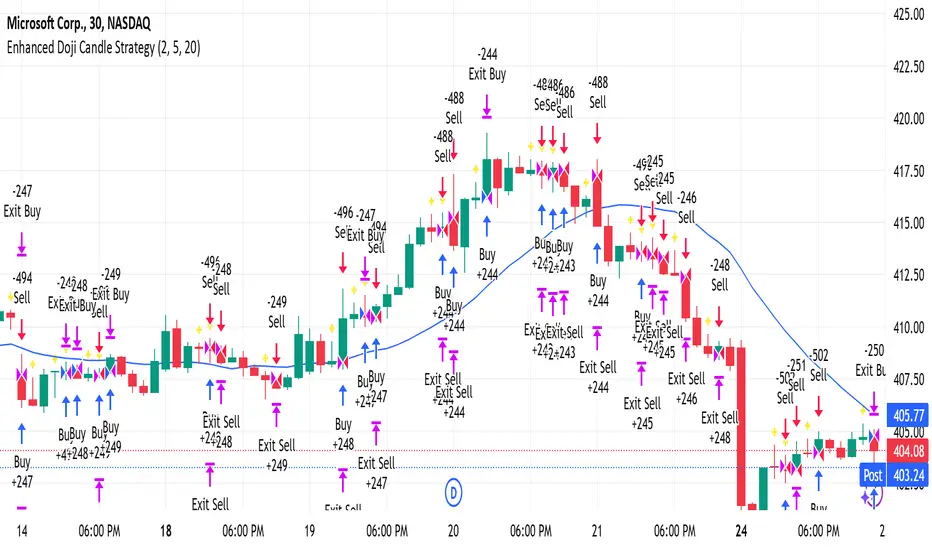
Enhanced Doji Candle StrategyYour trading strategy is a Doji Candlestick Reversal Strategy designed to identify potential market reversals using Doji candlestick patterns. These candles indicate indecision in the market, and when detected, your strategy uses a Simple Moving Average (SMA) with a short period of 20 to confirm the overall market trend. If the price is above the SMA, the trend is considered bullish; if it's below, the trend is bearish.
Once a Doji is detected, the strategy waits for one or two consecutive confirmation candles that align with the market trend. For a bullish confirmation, the candles must close higher than their opening price without significant bottom wicks. Conversely, for a bearish confirmation, the candles must close lower without noticeable top wicks. When these conditions are met, a trade is entered at the market price.
The risk management aspect of your strategy is clearly defined. A stop loss is automatically placed at the nearest recent swing high or low, with a tighter distance of 5 pips to allow for more trading opportunities. A take-profit level is set using a 2:1 reward-to-risk ratio, meaning the potential reward is twice the size of the risk on each trade.
Additionally, the strategy incorporates an early exit mechanism. If a reversal Doji forms in the opposite direction of your trade, the position is closed immediately to minimize losses. This strategy has been optimized to increase trade frequency by loosening the strictness of Doji detection and confirmation conditions while still maintaining sound risk management principles.
The strategy is coded in Pine Script for use on TradingView and uses built-in indicators like the SMA for trend detection. You also have flexible parameters to adjust risk levels, take-profit targets, and stop-loss placements, allowing you to tailor the strategy to different market conditions.
In den Scripts nach "bear" suchen
SuperTrend AI Oscillator StrategySuperTrend AI Oscillator Strategy
Overview
This strategy is a trend-following approach that combines the SuperTrend indicator with oscillator-based filtering.
By identifying market trends while utilizing oscillator-based momentum analysis, it aims to improve entry precision.
Additionally, it incorporates a trailing stop to strengthen risk management while maximizing profits.
This strategy can be applied to various markets, including Forex, Crypto, and Stocks, as well as different timeframes. However, its effectiveness varies depending on market conditions, so thorough testing is required.
Features
1️⃣ Trend Identification Using SuperTrend
The SuperTrend indicator (a volatility-adjusted trend indicator based on ATR) is used to determine trend direction.
A long entry is considered when SuperTrend turns bullish.
A short entry is considered when SuperTrend turns bearish.
The goal is to capture clear trend reversals and avoid unnecessary trades in ranging markets.
2️⃣ Entry Filtering with an Oscillator
The Super Oscillator is used to filter entry signals.
If the oscillator exceeds 50, it strengthens long entries (indicating strong bullish momentum).
If the oscillator drops below 50, it strengthens short entries (indicating strong bearish momentum).
This filter helps reduce trades in uncertain market conditions and improves entry accuracy.
3️⃣ Risk Management with a Trailing Stop
Instead of a fixed stop loss, a SuperTrend-based trailing stop is implemented.
The stop level adjusts automatically based on market volatility.
This allows profits to run while managing downside risk effectively.
4️⃣ Adjustable Risk-Reward Ratio
The default risk-reward ratio is set at 1:2.
Example: A 1% stop loss corresponds to a 2% take profit target.
The ratio can be customized according to the trader’s risk tolerance.
5️⃣ Clear Trade Signals & Visual Support
Green "BUY" labels indicate long entry signals.
Red "SELL" labels indicate short entry signals.
The Super Oscillator is plotted in a separate subwindow to visually assess trend strength.
A real-time trailing stop is displayed to support exit strategies.
These visual aids make it easier to identify entry and exit points.
Trading Parameters & Considerations
Initial Account Balance: Default is $7,000 (adjustable).
Base Currency: USD
Order Size: 10,000 USD
Pyramiding: 1
Trading Fees: $0.94 per trade
Long Position Margin: 50%
Short Position Margin: 50%
Total Trades (M5 Timeframe): 1,032
Visual Aids for Clarity
This strategy includes clear visual trade signals to enhance decision-making:
Green "BUY" labels for long entries
Red "SELL" labels for short entries
Super Oscillator plotted in a subwindow with a 50 midline
Dynamic trailing stop displayed for real-time trend tracking
These visual aids allow traders to quickly identify trade setups and manage positions with greater confidence.
Summary
The SuperTrend AI Oscillator Strategy is developed based on indicators from Black Cat and LuxAlgo.
By integrating high-precision trend analysis with AI-based oscillator filtering, it provides a strong risk-managed trading approach.
Important Notes
This strategy does not guarantee profits—performance varies based on market conditions.
Past performance does not guarantee future results. Markets are constantly changing.
Always test extensively with backtesting and demo trading before using it in live markets.
Risk management, position sizing, and market conditions should always be considered when trading.
Conclusion
This strategy combines trend analysis with momentum filtering, enhancing risk management in trading.
By following market trends carefully, making precise entries, and using trailing stops, it seeks to reduce risk while maximizing potential profits.
Before using this strategy, be sure to test it thoroughly via backtesting and demo trading, and adjust the settings to match your trading style.

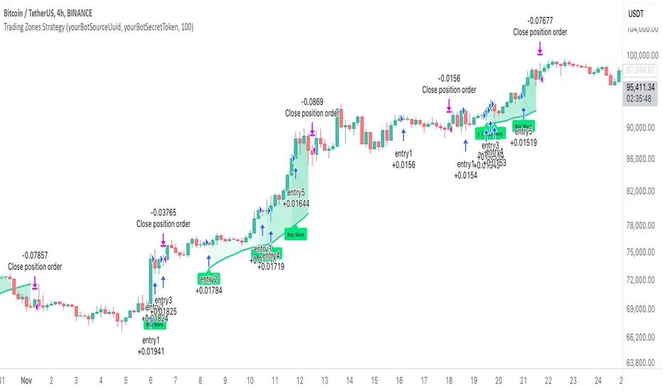
AO/AC Trading Zones Strategy [Skyrexio] Overview
AO/AC Trading Zones Strategy leverages the combination of Awesome Oscillator (AO), Acceleration/Deceleration Indicator (AC), Williams Fractals, Williams Alligator and Exponential Moving Average (EMA) to obtain the high probability long setups. Moreover, strategy uses multi trades system, adding funds to long position if it considered that current trend has likely became stronger. Combination of AO and AC is used for creating so-called trading zones to create the signals, while Alligator and Fractal are used in conjunction as an approximation of short-term trend to filter them. At the same time EMA (default EMA's period = 100) is used as high probability long-term trend filter to open long trades only if it considers current price action as an uptrend. More information in "Methodology" and "Justification of Methodology" paragraphs. The strategy opens only long trades.
Unique Features
No fixed stop-loss and take profit: Instead of fixed stop-loss level strategy utilizes technical condition obtained by Fractals and Alligator to identify when current uptrend is likely to be over. In some special cases strategy uses AO and AC combination to trail profit (more information in "Methodology" and "Justification of Methodology" paragraphs)
Configurable Trading Periods: Users can tailor the strategy to specific market windows, adapting to different market conditions.
Multilayer trades opening system: strategy uses only 10% of capital in every trade and open up to 5 trades at the same time if script consider current trend as strong one.
Short and long term trend trade filters: strategy uses EMA as high probability long-term trend filter and Alligator and Fractal combination as a short-term one.
Methodology
The strategy opens long trade when the following price met the conditions:
1. Price closed above EMA (by default, period = 100). Crossover is not obligatory.
2. Combination of Alligator and Williams Fractals shall consider current trend as an upward (all details in "Justification of Methodology" paragraph)
3. Both AC and AO shall print two consecutive increasing values. At the price candle close which corresponds to this condition algorithm opens the first long trade with 10% of capital.
4. If combination of Alligator and Williams Fractals shall consider current trend has been changed from up to downtrend, all long trades will be closed, no matter how many trades has been opened.
5. If AO and AC both continue printing the rising values strategy opens the long trade on each candle close with 10% of capital while number of opened trades reaches 5.
6. If AO and AC both has printed 5 rising values in a row algorithm close all trades if candle's low below the low of the 5-th candle with rising AO and AC values in a row.
Script also has additional visuals. If second long trade has been opened simultaneously the Alligator's teeth line is plotted with the green color. Also for every trade in a row from 2 to 5 the label "Buy More" is also plotted just below the teeth line. With every next simultaneously opened trade the green color of the space between teeth and price became less transparent.
Strategy settings
In the inputs window user can setup strategy setting:
EMA Length (by default = 100, period of EMA, used for long-term trend filtering EMA calculation).
User can choose the optimal parameters during backtesting on certain price chart.
Justification of Methodology
Let's explore the key concepts of this strategy and understand how they work together. We'll begin with the simplest: the EMA.
The Exponential Moving Average (EMA) is a type of moving average that assigns greater weight to recent price data, making it more responsive to current market changes compared to the Simple Moving Average (SMA). This tool is widely used in technical analysis to identify trends and generate buy or sell signals. The EMA is calculated as follows:
1.Calculate the Smoothing Multiplier:
Multiplier = 2 / (n + 1), Where n is the number of periods.
2. EMA Calculation
EMA = (Current Price) × Multiplier + (Previous EMA) × (1 − Multiplier)
In this strategy, the EMA acts as a long-term trend filter. For instance, long trades are considered only when the price closes above the EMA (default: 100-period). This increases the likelihood of entering trades aligned with the prevailing trend.
Next, let’s discuss the short-term trend filter, which combines the Williams Alligator and Williams Fractals. Williams Alligator
Developed by Bill Williams, the Alligator is a technical indicator that identifies trends and potential market reversals. It consists of three smoothed moving averages:
Jaw (Blue Line): The slowest of the three, based on a 13-period smoothed moving average shifted 8 bars ahead.
Teeth (Red Line): The medium-speed line, derived from an 8-period smoothed moving average shifted 5 bars forward.
Lips (Green Line): The fastest line, calculated using a 5-period smoothed moving average shifted 3 bars forward.
When the lines diverge and align in order, the "Alligator" is "awake," signaling a strong trend. When the lines overlap or intertwine, the "Alligator" is "asleep," indicating a range-bound or sideways market. This indicator helps traders determine when to enter or avoid trades.
Fractals, another tool by Bill Williams, help identify potential reversal points on a price chart. A fractal forms over at least five consecutive bars, with the middle bar showing either:
Up Fractal: Occurs when the middle bar has a higher high than the two preceding and two following bars, suggesting a potential downward reversal.
Down Fractal: Happens when the middle bar shows a lower low than the surrounding two bars, hinting at a possible upward reversal.
Traders often use fractals alongside other indicators to confirm trends or reversals, enhancing decision-making accuracy.
How do these tools work together in this strategy? Let’s consider an example of an uptrend.
When the price breaks above an up fractal, it signals a potential bullish trend. This occurs because the up fractal represents a shift in market behavior, where a temporary high was formed due to selling pressure. If the price revisits this level and breaks through, it suggests the market sentiment has turned bullish.
The breakout must occur above the Alligator’s teeth line to confirm the trend. A breakout below the teeth is considered invalid, and the downtrend might still persist. Conversely, in a downtrend, the same logic applies with down fractals.
In this strategy if the most recent up fractal breakout occurs above the Alligator's teeth and follows the last down fractal breakout below the teeth, the algorithm identifies an uptrend. Long trades can be opened during this phase if a signal aligns. If the price breaks a down fractal below the teeth line during an uptrend, the strategy assumes the uptrend has ended and closes all open long trades.
By combining the EMA as a long-term trend filter with the Alligator and fractals as short-term filters, this approach increases the likelihood of opening profitable trades while staying aligned with market dynamics.
Now let's talk about the trading zones concept and its signals. To understand this we need to briefly introduce what is AO and AC. The Awesome Oscillator (AO), developed by Bill Williams, is a momentum indicator designed to measure market momentum by contrasting recent price movements with a longer-term historical perspective. It helps traders detect potential trend reversals and assess the strength of ongoing trends.
The formula for AO is as follows:
AO = SMA5(Median Price) − SMA34(Median Price)
where:
Median Price = (High + Low) / 2
SMA5 = 5-period Simple Moving Average of the Median Price
SMA 34 = 34-period Simple Moving Average of the Median Price
The Acceleration/Deceleration (AC) Indicator, introduced by Bill Williams, measures the rate of change in market momentum. It highlights shifts in the driving force of price movements and helps traders spot early signs of trend changes. The AC Indicator is particularly useful for identifying whether the current momentum is accelerating or decelerating, which can indicate potential reversals or continuations. For AC calculation we shall use the AO calculated above is the following formula:
AC = AO − SMA5(AO) , where SMA5(AO)is the 5-period Simple Moving Average of the Awesome Oscillator
When the AC is above the zero line and rising, it suggests accelerating upward momentum.
When the AC is below the zero line and falling, it indicates accelerating downward momentum.
When the AC is below zero line and rising it suggests the decelerating the downtrend momentum. When AC is above the zero line and falling, it suggests the decelerating the uptrend momentum.
Now let's discuss the trading zones concept and how it can create the signal. Zones are created by the combination of AO and AC. We can divide three zone types:
Greed zone: when the AO and AC both are rising
Red zone: when the AO and AC both are decreasing
Gray zone: when one of AO or AC is rising, the other is falling
Gray zone is considered as uncertainty. AC and AO are moving in the opposite direction. Strategy skip such price action to decrease the chance to stuck in the losing trade during potential sideways. Red zone is also not interesting for the algorithm because both indicators consider the trend as bearish, but strategy opens only long trades. It is waiting for the green zone to increase the chance to open trade in the direction of the potential uptrend. When we have 2 candles in a row in the green zone script executes a long trade with 10% of capital.
Two green zone candles in a row is considered by algorithm as a bullish trend, but now so strong, that's the reason why trade is going to be closed when the combination of Alligator and Fractals will consider the the trend change from bullish to bearish. If id did not happens, algorithm starts to count the green zone candles in a row. When we have 5 in a row script change the trade closing condition. Such situation is considered is a high probability strong bull market and all trades will be closed if candle's low will be lower than fifth green zone candle's low. This is used to increase probability to secure the profit. If long trades are initiated, the strategy continues utilizing subsequent signals until the total number of trades reaches a maximum of 5. Each trade uses 10% of capital.
Why we use trading zones signals? If currently strategy algorithm considers the high probability of the short-term uptrend with the Alligator and Fractals combination pointed out above and the long-term trend is also suggested by the EMA filter as bullish. Rising AC and AO values in the direction of the most likely main trend signaling that we have the high probability of the fastest bullish phase on the market. The main idea is to take part in such rapid moves and add trades if this move continues its acceleration according to indicators.
Backtest Results
Operating window: Date range of backtests is 2023.01.01 - 2024.12.31. It is chosen to let the strategy to close all opened positions.
Commission and Slippage: Includes a standard Binance commission of 0.1% and accounts for possible slippage over 5 ticks.
Initial capital: 10000 USDT
Percent of capital used in every trade: 10%
Maximum Single Position Loss: -9.49%
Maximum Single Profit: +24.33%
Net Profit: +4374.70 USDT (+43.75%)
Total Trades: 278 (39.57% win rate)
Profit Factor: 2.203
Maximum Accumulated Loss: 668.16 USDT (-5.43%)
Average Profit per Trade: 15.74 USDT (+1.37%)
Average Trade Duration: 60 hours
How to Use
Add the script to favorites for easy access.
Apply to the desired timeframe and chart (optimal performance observed on 4h BTC/USDT).
Configure settings using the dropdown choice list in the built-in menu.
Set up alerts to automate strategy positions through web hook with the text: {{strategy.order.alert_message}}
Disclaimer:
Educational and informational tool reflecting Skyrex commitment to informed trading. Past performance does not guarantee future results. Test strategies in a simulated environment before live implementation
These results are obtained with realistic parameters representing trading conditions observed at major exchanges such as Binance and with realistic trading portfolio usage parameters.
ATR SuperTrend - IonJauregui-ActivTradesEste script en Pine Script utiliza el indicador SuperTrend basado en el ATR para identificar tendencias y generar señales de compra y venta.
¿Cómo funciona?
Detecta la volatilidad con el ATR para calcular niveles dinámicos de soporte y resistencia.
Dibuja la tendencia:
Línea verde: Tendencia alcista.
Línea roja: Tendencia bajista.
Genera señales de trading:
Compra cuando la tendencia pasa de bajista a alcista.
Venta cuando cambia de alcista a bajista.
Opera de forma automática:
Abre posiciones según las señales.
Establece stop loss y take profit para gestionar el riesgo.
Este indicador ayuda a seguir la tendencia y automatizar operaciones, filtrando el ruido del mercado.
**********************************************************
This Pine Script uses the SuperTrend indicator based on ATR to identify trends and generate buy and sell signals.
How it works:
Detects volatility with ATR to calculate dynamic support and resistance levels.
Plots the trend:
Green line: Bullish trend.
Red line: Bearish trend.
Generates trading signals:
Buy when the trend switches from bearish to bullish.
Sell when it switches from bullish to bearish.
Trades automatically:
Opens positions based on the signals.
Sets stop loss and take profit to manage risk.
This indicator helps follow the trend and automate trades, filtering out market noise.

Liquidity Trading Algorithm (LTA)
The Liquidity Trading Algorithm is an algorithm designed to provide trade signals based on
liquidity conditions in the market. The underlying algorithm is based on the Liquidity
Dependent Price Movement (LDPM) metric and the Liquidity Dependent Price Stability (LDPS)
algorithm.
Together, LDPM and LDPS demonstrate statistically significant forecasting capabilities for price-
action on equities, cryptocurrencies, and futures. LTA takes these liquidity measurements and
translates them into actionable insights by way of entering or exiting a position based
on the future outlooks, as measured by the current liquidity status.
The benefit of LTA is that it can incorporate these powerful liquidity measurements into
actionable insights with several features designed to help you tailor LTA's behavior and
measurements to your desired vantage point. These customizable features come by the way of determining LTA's assessment style, and additional monitoring systems for avoiding bear and bull traps, along with various other quality of life features, discussed in more detail below.
First, a few quick facts:
- LTA is compatible on a wide array of instruments, including Equities, Futures, Cryptocurrencies, and Forex.
- LTA is compatible on most intervals in so long as the data can be calculated appropriately,
(be sure to do a backtest on timescales less than 1-minue to ensure the data can be computed).
- LTA only measures liquidity at the end of the interval of the chart chosen, and does not respond to conditions during the candle interval, unless specified (such as with `Stops`).
- LTA is interval-dependent, this means it will measure and behave differently on different
intervals as the underlying algorithms are dependent on the interval chosen.
- LTA can utilize fractional share sizing for cryptocurrencies.
- LTA can be restricted to either bullish or bearish indications.
- Additional Monitoring Systems are available for additional risk mitigation.
In short, LTA is a widely applicable, unique algorithm designed to translate liquidity measurements into liquidity insights.
Before getting more into the details, here is a quick list of the main features and settings
available for customization:
- Backtesting Start Date: Manual selection of the start date for the algorithm during backtesting.
- Assessment Style: adjust how LDPM and LDPS measure and respond to changes in liquidity.
- Impose Wait: force LTA to wait before entering or exiting a position to ensure conditions have remained conducive.
- Trade Direction Allowance: Restrict LTA to only long or only short, if desired.
- Position Sizing Method: determine how LTA calculates position sizing.
- Fractional Share Sizing: allow LTA to calculate fractional share sizes for cryptocurrencies
- Max Size Limit: Impose a maximum size on LTA's positions.
- Initial Capital: Indicate how much capital LTA should stat with.
- Portfolio Allotment: Indicate to LTA how much (in percentages) of the available balance should be considered when calculating position size.
- Enact Additional Monitoring Systems: Indicate if LTA should impose additional safety criteria when monitoring liquidity.
- Configure Take Profit, Stop-Loss, Trailing Stop Loss
- Display Information tables on the current position, overall strategy performance, along
with a text output showing LTA's processes.
- Real-time text output and updates on LTA's inner workings.
Let's get into some more of the details.
LTA's Assessment Style
LTA's assessment style determines how LTA collects and responds to changing data. In traditional terms, this is akin to (but not quite exactly the same as) the sensitivity versus specificity spectrum, whereby on one end (the sensitive end), an algorithm responds to changes in data in a reactive manner (which tends to lower its specificity, or how often it is correct in its indications), and on the other end, the opposite one, the algorithm foresakes quick changes for longevity of outlook.
While this is in part true, it is not a full view of the underlying mechanisms that changing the assessment style augments. A better analogy would be that the sensitive end of the spectrum (`Aggressive`) is in a state such that the algorithm wants to changing its outlooks, and as such, with changes in data, the algorithm has to be convinced as to why that is not a good idea to change outlooks, whereas the the more specific states (`Conservative`, `Diamond`) must be convinced that their view is no longer valid and that it needs to be changed.
This means the `Aggressive` and the `Diamond` settings fundamentally differ not just in their
data collection, but also in the data processing such that the `Aggressive` decision tree has to
be convinced that the data is the same (as its defualt is that it has changed),
and the `Diamond` decision tree has to be convinced that the data is not the same, and as such, the outlook need changed.
From there, the algorithm cooks through the data and determines to what the outlook should be changed to, given the current state of liquidity.
`Balanced` lies in the middle of this balance, attempting to balance being open to new ideas while not removing the wisdom of the past, as it were.
On a scale of most `sensitive` to most `specific`, it is as follows: `Aggressive`, `Balanced`,
`Conservative`, `Diamond`.
Functionally, these different modes can help in different liquidity environments, as certain
environments are more conducive to an eager approach (such as found near `Aggressive`) or are more conducive to a more conservative approach, where sudden changes in liquidity are known to be short-lived and unremarkable (such as many previously identified bull or bear traps).
For instance, on low interval views, it can often-times be beneficial to keep the algorithm towards the `Sensitive` end, since on the lower-timeframes, the crosswinds can change quite dramatically; whereas on the longer intervals, it may be useful to maintain a more `Specific` algorithm (such as found near `Diamond` mode) setting since longer intervals typically lend themselves to longer time-horizons, which themselves typically lend themselves to "weathering the storm", as it were.
LTA's Assessment Style is also supported by the Additional Monitoring Systems which works
to add sensitivity without sacrificing specificity by enacting a separate monitoring system, as described below.
Additional Monitoring Systems
The Additional Monitoring System (AMS) attempts to add more context to any changes in liquidity conditions as measured, such that LTA as a whole will have an expanded view into any rapidly changing liquidity conditions before these changes manifest in the traditional data streams. The ideal is that this allows for early exits or early entrances to positions "a head of time".
The traditional use of this system is to indicate when liquidity is suggestive of the end of a particular run (be it a bear run or a bull run), so an early exit can be initiated (and thus,
downside averted) even before the data officially showcase such changes. In such cases (when AMS becomes activated), the algorithm will signal to exit any open positions, and will restrict the opening of any new positions.
When a position is exited because of AMS, it is denoted as an `Early Exit` and if a position is prevented from being entered, the text output will display `AM prevented entry...` to indicate that conditions are not meeting AMS' additional standards.
The algorithm will wait to make any actions while `AMS` is `active` and will only enter into a new position once `AMS` has been `deactivated` and overall liquidity conditions are appropriate.
Functionally, the benefits of AMS translate to:
- Toggeling AMS on will typically see a net reduction in overall profitability, but
- AMS will typically (almost always) reduce max drawdown,
an increases in max runup, and increase return-over-maxdrawdown, and
- AMS can provide benefit for equities that experience a lot of "traps" by navigating early
entrance and early exits.
So in short, AMS is way of adding an additional level of liquidity monitoring that attempts to
exit positions if conditions look to be deteriorating, and to enter conditions if they look to be
improving. The cost of this additional monitoring, however, is a greater number of trades indicated, and a lower overall profitability.
Impose Wait
Note: `Impose Wait` will not force Take Profit, Stop Loss, or Trailing Stop Loss to
wait.
LTA can be indicated to `wait` before entering or exiting a position if desired. This means that if conditions change, whereas without a `wait` imposed, the algorithm would immediately indicate this change via a signal to alter the strategy's position, with a `wait` imposed, the algorithm will `wait` the indicated number of bars, and then re-check conditions before proceeding.
If, while waiting, conditions change to a state that is no longer compatible with the "order-in-
waiting", then the order-in-waiting is removed, and the counts reset (i.e.: conditions must remain favorable to the intended positional change throughout the wait period).
Since LTA works at the end-of-intervals, there is an inherently "built-in" wait of 1 bar when
switching directly from long to short (i.e.: if a full switch is indicated, then it is indicated as
conditions change -> exit new position -> wait until -> check conditions ->
enter new position as indicated). Thus, to impose a wait of `1 bar` would be to effectively have a total of two candles' ends prior to the entrance of the new position).
There are two main styles of `Impose Wait` that you can utilize:
- `Wait` : this mode will cause LTA to `wait` when both entering and exiting a position (in so long as it is not an exit signaled via a Take Profit, Stop Loss or Trailing Stop Loss).
- `Exit-Wait` : This mode will >not< cause LTA to `wait` if conditions require the closing of a position, but will force LTA to wait before entering into a position.
Position:
In addition to the availability to restrict LTA to either a long-only or short-only strategy, LTA
also comprises additional flexibility when deciding on how it should navigate the markets with
regards to sizing. Notably, this flexibility benefits several aspects of LTA's existence, namely the ability to determine the `Sizing Method`, or if `Fractional Share Sizing` should be employed, and more, as discussed below.
Position Sizing Method
There are two main ways LTA can determine the size of a position. Either via the `Fixed-Share` choice, or the `Fixed-Percentage` choice.
- `Fixed-Share` will use the amount indicated in the `Max Sizing Limit` field as the position size, always.
Note: With `Fixed-Share` sizing, LTA will >not< check if the balance is sufficient
prior to signaling an entrance.
- `Fixed-Percentage` will use the percentage amount indicated in the `Portfolio Allotment` field as the percentage of available funds to use when calculating the position size. Additionally, with the `Fixed-Percentage` choice, you can set the `Max Sizing Limit` if desired, which will ensure that no position will be entered greater than the amount indicated in the field.
Fractional Share Sizing
If the underlying instrument supports it (typically only cryptocurrencies), share sizing can be
fractionalized. If this is done, the resulting positin size is rounded to `4 digits`. This means any
position with a size less than `0.00005` will be rounded to `0.0000`
Note: Ensure that the underlying instrument supports fractional share sizing prior
to initiating.
Max Sizing Limit
As discussed above, the `Max Sizing Limit` will determine:
- The position size for every position, if `Sizing Method : Fixed-Share` is utilized, or
- The maximum allowed size, regardless of available capital, if `Sizing Method : Fixed-Percentage` is utilized.
Note: There is an internal maximum of 100,000 units.
Initial Capital
Note: There are 2 `Initial Capital` settings; one in LTA's settings and one in the
`Properties` tab. Ensure these two are the same when doing backtesting.
The initial capital field will be used to determine the starting balanace of the strategy, and
is used to calculate the internal data reporting (the data tables).
Portfolio Allotment
You can specify how much of the total available balance should be used when calculating the share size. The default is 100%.
Stops
Note: Stops over-ride `AMS` and `Impose Wait`, and are not restricted to only the
end-of-candle and will occur instantaneously upon their activation. Neither `AMS` nor `Impose Wait` can over-ride a signal from a `Take-Profit`, `Stop-Loss`, or a `Trailing-Stop Loss`.
LTA enhouses three stops that can be configured, a `Take-Profit`, a `Stop-Loss` and a `Trailing-Stop Loss`. The configurations can be set in the settings in percent terms. These exit signals will always over-ride AMS or any other restrictions on position exit.
Their configuration is rather standard; set the percentages you want the signal to be sent at and so it will be done.
Some quick notes on the `Trailing-Stop Loss`:
- The activation percentage must be reached (in profits) prior to the `Traililng-Stop Loss`
from activating the downside protection. For example, if the `Activation Percentage` is 10%, then unless the position reaches (at any point) a 10% profit, then it will not signal any exits on the downside, should it occur.
- The downside price-point is continuously updated and is calculated from the maximum profit reached in the given position and the loss percentage placed in the appropriate field.
Data Tables and Data Output
LTA provides real-time data output through a variety of mechanisms:
- `Position Table`
The `Position Table` displays information about the current position, including:
> Position Duration : how long the position has been open for.
> Indicates if the side is Long or Short, depending on if it is long or short.
> Entry Price: the price the position was entered at.
> Current Price (% Dif): the current price of the underlying and the %-difference between the entry price and the current price.
> Max Profit ($/%): the maximum profit reached in $ and % terms.
> Current PnL ($/%) : the current PnL for the open position.
- `Performance Table`
The `Performance Table` displays information regarding the overall performance of the algorithm since its `Start Date`. These data include:
> Initial Equity ($): The initial equity the algorithm started with.
> Current Equity ($): The current total equity of the account (including open positions)
> Net Profits ($|%) : The overall net profit in $ and % terms.
> Long / Short Trade Counts: The respective trade counts for the positions entered.
> Total Closed Trades: The running sum of the number of trades closed.
> Profitability: The calculation of the number of profitable trades over the total number of
trades.
> Avg. Profit / Trade: The calculation of the average profit per trade in both $ and % terms.
> Avg. Loss / Trade: The calculation of the average loss per trade in both $ and % terms.
> Max Run-Up: The maximum run-up the algorithm has seen in both $ and % terms.
> Max Drawdown: The maximum draw-down the algorithm has seen in both $ and % terms.
> Return-Over-Max-Drawdown: the ratio of the maximum drawdown against the current net profits.
- `Text Output`
LTA will output, if desired, signals to the text output field every time it analysis or performs and action. These messages can include information such as:
"
08:00:00 >> AM Protocol activated ... exiting position ...
08:00:00 >> Exit Order Created for qty: 2, profit: 380 (4.34%)
...
09:30:00 >> Checking conditions ...
09:30:00 >> AM protocol prevented entry ... waiting ...
"
This way, you can keep an eye out on what is happening "under the hood", as it were.
LTA will produce a message at the end of its assessment at the end of each candle interval, as well as when a position is exited due to a `Stop` or due to `AMS` being activated.
Additionally, the `Text Output` includes a initial message, but for space-constraints, this
can be toggled off with the `Blank Text Output` option within LTA's configurations.
For additional information, please refer to the Author's Instructions below.

DAILY Supertrend + EMA Crossover with RSI FilterThis strategy is a technical trading approach that combines multiple indicators—Supertrend, Exponential Moving Averages (EMAs), and the Relative Strength Index (RSI)—to identify and manage trades.
Core Components:
1. Exponential Moving Averages (EMAs):
Two EMAs, one with a shorter period (fast) and one with a longer period (slow), are calculated. The idea is to spot when the faster EMA crosses above or below the slower EMA. A fast EMA crossing above the slow EMA often suggests upward momentum, while crossing below suggests downward momentum.
2. Supertrend Indicator:
The Supertrend uses Average True Range (ATR) to establish dynamic support and resistance lines. These lines shift above or below price depending on the prevailing trend. When price is above the Supertrend line, the trend is considered bullish; when below, it’s considered bearish. This helps ensure that the strategy trades only in the direction of the overall trend rather than against it.
3. RSI Filter:
The RSI measures momentum. It helps avoid buying into markets that are already overbought or selling into markets that are oversold. For example, when going long (buying), the strategy only proceeds if the RSI is not too high, and when going short (selling), it only proceeds if the RSI is not too low. This filter is meant to improve the quality of the trades by reducing the chance of entering right before a reversal.
4. Time Filters:
The strategy only triggers entries during user-specified date and time ranges. This is useful if one wants to limit trading activity to certain trading sessions or periods with higher market liquidity.
5. Risk Management via ATR-based Stops and Targets:
Both stop loss and take profit levels are set as multiples of the ATR. ATR measures volatility, so when volatility is higher, both stops and profit targets adjust to give the trade more breathing room. Conversely, when volatility is low, stops and targets tighten. This dynamic approach helps maintain consistent risk management regardless of market conditions.
Overall Logic Flow:
- First, the market conditions are analyzed through EMAs, Supertrend, and RSI.
- When a buy (long) condition is met—meaning the fast EMA crosses above the slow EMA, the trend is bullish according to Supertrend, and RSI is below the specified “overbought” threshold—the strategy initiates or adds to a long position.
- Similarly, when a sell (short) condition is met—meaning the fast EMA crosses below the slow EMA, the trend is bearish, and RSI is above the specified “oversold” threshold—it initiates or adds to a short position.
- Each position is protected by an automatically calculated stop loss and a take profit level based on ATR multiples.
Intended Result:
By blending trend detection, momentum filtering, and volatility-adjusted risk management, the strategy aims to capture moves in the primary trend direction while avoiding entries at excessively stretched prices. Allowing multiple entries can potentially amplify gains in strong trends but also increases exposure, which traders should consider in their risk management approach.
In essence, this strategy tries to ride established trends as indicated by the Supertrend and EMAs, filter out poor-quality entries using RSI, and dynamically manage trade risk through ATR-based stops and targets.

LETF Leveraged Edge Strategy v1.5Overview
The strategy is based on Stochastics to detect trends and then makes Buys and Sell based on custom entry and exit criteria as described below in the Execution Logic Rules section. It will NOT work with standard Stochastics.
This is not a standard Stochastics implementation. It has been customized and modified, and does not match any widely known Stochastics variations (like Fast, Slow, or Full Stochastics) in its smoothing and iterative calculation process with:
• A unique smoothing mechanism.
• Iterative calculations.
• Additional conditional logic for strategy execution.
This strategy is designed to focus on volatile, liquid leveraged ETFs to capture gains equal to or better than Buy and Hold, and mitigate the risk of trading with a goal of reducing drawdown to a lot less than Buy and Hold. It has had successful backtest performance to varying degrees with TQQQ, SOXL, FNGU, TECL, FAS, UPRO, NAIL and SPXL. Results have not been good on other LETFs that have been backtested.
Performance
In this backtest the Net Profit shows to be $4,561 or 45.61%. Considering the initial order size was $1,000 I have to wonder if the Strategy Tester is calculating this correctly. The Strategy Tester Performance Summary shows the Buy and Hold Return at $61,165 or 611.7%. Based on calculating the price of the last shares sold, less the price paid, times the number of initial shares purchased, my math shows the Buy and Hold Gain at $4,572 or about equal with the strategy performance in this case. The Performance Summary also states the strategy had a Max DD of 3.46% which I believe is incorrect. Based on other backtests I’ve done, I believe the strategy drawdown here was closer to 28.4% and the Buy and Hold Drawdown at 82.7%. I manually calculated the Buy and Hold drawdown.
How it Works
The author provides training and support resource materials for this at his website. The strategy execution logic is driven by these rules:
Execution Logic Rules
Buy the LETF When:
BR #1a) The Daily Fast Line (FL) crosses above the Daily Slow Line (SL) and the FL is between the Low (L*) and High (H*) Range set (often referred to as Oversold and Overbought Lines). This can execute (Buy) any trading day of the week.
BR #1b) Re-Buy the next day after any Stop or Take Profit Sell if the Buy Rule condition is true (FL is above SL), if not, remain in cash and wait for the next Buy Signal.
Sell the LETF When:
SR #1a) The Daily Fast Line (FL) crosses below Daily Slow Line (SL) within the Low (L*) and High (H*) Range (often referred to as Oversold and Overbought Lines). “Crossunder Range Exit” This can execute (Sell) any trading day of the week.
SR #1b) If the (FL) crosses Below the SL above the Exit Level*, wait. Only Sell if the FL drops down below the Exit Level* “Crossunder Level Exit” This can execute (Sell) any trading day of the week.
SR #2a) Sell at the open any day the gap-down price is at or below the 1-Day Stop%*, based on previous day’s closing price (Execute on the day it happens.)
SR #2b) Sell intraday any day the price is at or below the 1-Day Stop %*, based on previous day’s closing price (Execute on the day it happens.)
SR #3a) Sell at the open any day the price is at or below the Trailing Stop %*, based on highest intraday price since Buy date (Execute on the day it happens.)
SR #3b) Sell intraday any day the price is at or below the Trailing Stop%*, based on highest intraday price since Buy date (Execute on the day it happens.)
SR #4) Sell any day when the opening price exceeds, or intraday price meets the Profit Target % price* (Execute on the day it happens.)
SR #5) After each Sell go to Rule BR #1b to determine if a Re-Buy should occur the next day, or stay in cash until next Buy Signal
Settings:
Properties Tab – Initial Capital has been set to $10,000 and order size 10% of Equity, 0.1% commission and 3 Ticks for slippage. Net order size is $1,000
Input Tab:
Stochastic
Timeframe is selected to Daily or Weekly based on preference. Daily has more trades, but on average higher profitability.
Type: Proprietary (best selection for most LETFs, but a few will work better with the Full selection
%k Length 20, %K Smoothing 14, %D Smoothing (many LETFs work better with a specific Stoch setting, often each different) A List of these is provided for your starting point.
Trade Settings
Direction: Longs (This strategy only works on the Long side)
Stop Type: Trailing is recommended, but Fixed is an option.
Stop % (based on user risk tolerance)
PD Stop % (Suggest start at 5%. Based on volatility of LETF and is a stop percentage from prior day’s close. Designed to protect against sudden market volatility. Will need to balance between strategy performance and user risk tolerance)
Profit Target: User preference. (I can help with suggestions based on historical performance)
Entry/Exit Conditions
Enter on Tie: Default Checked – if a Fast line crosses a Slow line for a Buy signal, but doesn’t do so in the range set, this will trigger if it crosses at a tie.
Renter – Default Checked – If stopped out of a position, this tells the strategy to re-buy the position the next day if the conditions are still positive.
Exit Level: This is a exit level for a Fast cross below a Slow line that takes place above the Sell Range, but only happens if the Fast continues down to the level set. These usually don’t happen often, but can have a significant impact on performance. Unfortunately, it’s a trial and error process starting with 90 and working down to see if there’s any positive impact.
Trade Range
Buy Range: Start at typical 20 to 80. Expand the low end down first to check on performance impact. Normally a wide buying range is better for performance.
Sell Range: Start at 20 to 80 and tighten gradually to see performance impact. In some cases a very tight sell range does better. I have worked on our primary LETFs for many months to determine ranges for each that typically produce better results.
External Indicator: Some additional indicators have a positive impact on the strategy performance by increasing P/l, reducing drawdown and reducing the number of trades. This is not always the case and each LETF and time period for the LETF will have a bearing on whether the secondary indicator will help or not. Two that have helped are the MACD Histogram, and the Sloe-Velocity Indicator by Kamleshkumar43. Sometimes a couple of different indicators will have a positive impact, then it’s a personal preference which you pick to use with the strategy.
Since this strategy is focused on a very narrow selection of liquid LETFs, I have a lot of experience experimenting with the settings for the primary ones and can suggest things that will help. Additional training on the rules, working with the settings, and mitigating some of the negative trades during choppy markets is available at the website.
Chart
The strategy can be selected to use either a Daily or Weekly version of stochastic. This is important because the characteristics are different while still generating very good gains and minimal drawdowns. Generally, the daily stochastic will have a greater number of, and certainly more frequent, trades than the weekly stochastic. However, on average the daily version of the stochastic will generates greater profitability.
The Settings tabs have tooltip icons that will assist in inputting values that correspond to the written rules for the strategy, and some include specific rule detail.
Buying
The strategy generates Buy signals with the Fast line crossing over the Slow line within a “Buy Range” which is adjusted based on volatility of the leveraged ETF. This is unique in that a default is set for these entries to occur if the values are tied and doesn’t need to be within the high and low range if that occurs. The trader can select in the strategy for this to occur the same day, if he’s selected a Daily Stochastic timeframe, or at the end of the trading week if he’s selected a Weekly stochastic timeframe. The volatility of a leveraged ETF will sometimes cause a shake-out exit, a trailing stop can be hit, or there can be an exit based on taking a profit. A big part of the timing challenge was how to handle these. The strategy normally (set as a default) will immediately re-buy the next day only if the original buy conditions are still true. This helps capture gains when conditions are still favorable but keeps the trader out when they’re not.
Selling
Exits are handled in several ways. The strategy will exit if there is a fast line cross below a slow line within the “range”. The range is adjusted based on volatility of the leveraged ETF. The exit occurs at the close of the day if the trader has selected to use a Daily stochastic setting. The exit will occur at the end of the trading week if the trader has chosen a weekly stochastic strategy. The trader will set a level based on the instrument and volatility for another exit type. The level will sometimes coincide with the range exit high level but does not need to. If a fast line crosses down through a slow line above the level set, and then comes down to that level, the strategy will exit the position.
Another unique aspect of the strategy is the PD Stop setting. This is short for “Prior Day”, Rather than a normal stop based on the price paid for a position, the PD Stop is based on a percentage drop from the previous day’s closing price. This helps account for the volatility of the leveraged ETF and will cause an exit quickly if there’s a market, or index moving event. This helps capture gains and reduce risk should there be continued pullback.
Exits will also occur based on setting a trailing stop level and profit taking level. These are adjusted based on the leveraged ETFs volatility and historical performance.
Limitations
Choppy, or sideways markets are the most prone to poor performance and potential for being stopped out multiple times. If stopped out two consecutive times, make sure you’re monitoring market health and there are clear signs of a new uptrend such as a 10D and 21D MA in proper alignment and moving up. If you get a Buy signal from the strategy and you’re not confident yet about market and price direction then it’s fine to wait a day, or several days, to enter after the Buy signal when you have greater confidence about market direction. The author can help with a short list of tactical rules developed for these sideways or choppy markets.
This strategy has proven successful backtest results with a very limited set of LETFs as discussed earlier. The author does not know if it will prove successful with any others, or other types of ETFs such as 2X or plain ETFs. A lot more testing needs to be done.
The strategy buys and sells , excluding stops or take profit, at the market close. It can be very challenging to enter an order at market close.
Disclaimer
Please remember that past performance may not be indicative of future results.
Due to various factors, including changing market conditions, the strategy may no longer perform as well as in historical backtesting. This post and the script do not provide any financial advice and are for educational and entertainment purposes only.

TheHorsyAlgoPROThe Horsy algo is an automated strategy that uses any minute Higher timeframe range as reference and search for a purge of liquidity on the HTF high or low where buyside or sell side liquidity is, the algo only search this at specific desired times that can be configured according to the time you usually trade, the strategy is known as Turtle soup purge and reverse or lately as CRT.
Why is useful?
The purpose of this Algorithm is to help turtle soup traders to quickly identify when the market is likely to reverse the algo evaluates if the opportunity is worth it, base on risk reward and other desired filters. Also this strategy can help to quickly backtest the trader strategy it can be configured in different timeframes and adapt to the trader personality, they can easily see the results and statistics and notice if its profitable or not.
This algo is useful for intraday traders looking for a purge and reverse at a key times and at key HTF price levels this only looks the previous HTF highs and lows but is important to also monitor Order blocks, FVGs, gaps, or wicks to have the best results.
How it works and how it does it?
The Horsy algo simply Jumps from one type of liquidity to another one buyside to sell side or vice versa. In order for the algo to trigger an entry it has to meet these conditions
1. Take HTF liquidity, trade above a HTF high or below a HTF low in the selected time window
2. Make a change in the state of delivery with a close below the previous candle low for shorts and close above previous candle high for longs.
3. Allow for a reasonable risk reward, it will use the highest high for shorts and the lowest low for longs. The default take profit is the opposite side of the range.
4. Validate others user filters this include enter only trades aligned with the HTF bias, or trades aligned with the LTF bias or booth. The algo have the option to enter only premium and discount entries. And finally, an option to allow for different contract sizes depending of the maximum percent of the account we want to risk default is 1%. For this last option is important to check the initial balance and leverage are configured correctly, is disable by default because it requires more capital to perform well.
We can see the algo performing in the picture below with a short trade, notice there are some white lines, they are the high or the low of HTF candle that start generating inside candles in the HTF meaning a possible consolidation. The algo plots the HTF ranges in a shaded boxes as you can see below
The HTF bias as you can see in the picture is calculated based on the last close of the HTF meaning close above previous HTF high is bullish close below previous HTF low is bearish. This HTF bias level is also the last HTF mid-price or 50%. By default, this line is enabled.
The LTF bias is calculated based on the range created from the expansion outside the previous HTF range is also the mid-price. If the LTF close above previous HTF high is bullish and if the LTF close below previous HTF low is bearish. By default this LTF bias line is disable.
This strategy includes an original and personal developed code that uses dealing ranges to recognize if the market is expanding, retracing, reversing or consolidating. This allow the algo to exit the position when it detects a retracement or at the end of the expansion. This is the default exit type.
You can monitor the previous dealing ranges created in history with an option than can be enable, by default is disable, this ranges are created after price takes buyside and then sell side or vice versa. So this dealing ranges can be useful also to identify minor pools of liquidity and premium and discount in the lower timeframe.
The picture below is a long example, the exit in this case is just at the high of the range. The normal take profit is in a blue line for longs.
How to use it?
First select the desired HTF timeframe recommended is from 30min to 240min then you setup the chart on the lower timeframe you want to trade recommended is from 1min to 15min to enter. By default This strategy is designed to work for intraday during key times when price take stops and then moves quickly away from them. You can select as much as 6 different times or just one. After you select the desired time window where the algo will look for the purge and reverse, They are highlighted in the candles that change colors excluding the gray ones that indicates consolidation.
Then the Algo allow to performs several additional filters in the entries you can select if you want to trade only longs or shorts trades, you can select when to move the stop loss to Break even. In deviations of the risk or you can just select to remove risk when price hits the 50% of previous HTF range.
You can select the minimum desired risk reward of the trade before is allow to be taken. Once is configured correctly the algo should trigger signals with a triangle up or down plus the strategy entry.
At the beginning of the picture there are some blue lines in the HTF high low and close, this is to easily identify that the market is in the Asia session, the time can be configured by the user, these lines are normally gray.
On the right top of the screen you can see some statistics about the strategy how many trades it took, ARR is an approximated value of the accumulated total risk reward of all the trades when they get closed in the simulation.
Profit factor and percent profitable are also shown should be green it means that the strategy makes money over time. But apart from that is important to notice how it makes money it is stable over time? it is a roller coaster? that why I Include this other measurements MxcsTps is the maximum consecutives take profits and Mxcsls is the maximum consecutive stop losses it takes, the slash number after it is the consecutive Break evens. So this way you know what to expect and what is normal in the strategy.
The algo shows all the times the stop loss, take profit and break even level if enable in the colored red lines for short and blue lines for longs. You can also select how price will manage the profit or stoploss point meaning that you can choose to wait for the candle to close to invalidate your idea or to take profit. This is good to avoid liquidity sweeps but can also lead to mayor loses if the idea is wrong. The default setting is to close the trade when price takes the high or low where the stoploss is, the take profit is taken after a retracement to allow to profit on expansions. You can select also to exit on a reversal if you want to ride all the move. This last option has to be used with caution because sometimes price just retrace or reverse very fast decreasing the trade profit and overall strategy performance.
The algo have the option to use standard deviation from the normal risk if you prefer to prevent liquidity sweeps near the stop level this make wider stops but can lead to increased loses so it has to be used carefully.
Below is a picture that show the entry stop and take profit levels with an exit on a retracement activated.
Strategy Results
The backtesting results are obtained simulating a 2000usd account in the Micro Nasdaq using 1 contract per trade. Commission are set to 2usd per contract, slippage to 1tick. You can see in list of trades we are not risking more than 1 % percent of the account. The backtested range is from august to November 2024. This strategy doesn’t generate too much trades because of the time filters and conditions that has to be meet to take an entry but you can see the results of the last 4months with the available data that are around 32 trades.
The default settings for this strategy is HTF as 240min designed to work on a LTF 5min chart, the default purge times are 245-300, 745-800, 845-900, 1045-1100 and 1245-1300 UTC-4, the algo will look for shorts or longs, with a minimum risk reward of 2.0. With an additional filter of the HTFBias. The take profit is by default taken on the first retracement after hitting the target. The default settings are optimized to work on the Nasdaq or Spy, but can also perform well in other assets with the correct adjustments.
Remember entries constitute only a small component of a complete winning strategy. Other factors like risk management, position-sizing, trading frequency, trading fees, and many others must also be properly managed to achieve profitability. Past performance doesn’t guarantee future results. To really take advantage of this strategy you have to study turtle soup and the HTF key levels use this only as a confirmation that your overall idea will play out and use it to backtest your model.
Summary of features
·Adaptable strategy to different HTF timeframes from 1-1440min
· Select up to 6 different purge time windows UTC-4, UTC-5
· Choose desired Risk Reward per trade
· Easily see the HTF high low close and 50% key levels in the LTF
· Identify HTF consolidations that generate key major liquidity pools
· HTF/LTF bias filters to trade in favor of the big trend or in sync
· Shaded boxes that indicate if the market is bullish, bearish or consolidating
· See the current midpoint of the last expansion move
· Optimal trade entry filter to trade only in a discount or premium
· Customizable trade management take profit, stop, breakeven level
· Option to exit on a close, retracement or reversal after hitting the take profit level
· Option to exit on a close or reversal after hitting stop loss
· Configurable breakeven point with standard deviations or at 50% of the HTF
· Calculate different contract sizes depending of a percentage of the initial balance
· Standard deviations from normal risk can be used to prevent liquidity sweeps
· See dealing ranges history to check minor pools of liquidity and premium or discount
· Dashboard with instant statistics about the strategy current settings

Universal Trend Following Strategy | QuantumRsearchUniversal All Assets Strategy by Rocheur
The Universal All Assets Strategy is a cutting-edge, trend-following algorithm designed to operate seamlessly across multiple asset classes, including equities, commodities, forex, and cryptocurrencies. This strategy leverages the power of eight unique indicators, offering traders robust, adaptive signals. Its dynamic logic, combined with a comprehensive risk management framework, allows for precision trading in a variety of market conditions.
Core Methodologies and Features
1. Eight Integrated Trend Indicators
At the heart of the Universal All Assets Strategy are eight sophisticated trend-following indicators, each designed to capture different facets of market behavior. These indicators work together to provide a multi-dimensional analysis of price trends, filtering out noise and reacting only to significant movements:
Directional Moving Averages : Tracks the primary market trend, offering a clear indication of long-term price direction, ideal for identifying sustained upward or downward movements.
Smoothed Moving Averages : Reduces short-term volatility and noise to reveal the underlying trend, enhancing signal clarity and helping traders avoid reacting to temporary price spikes.
RSI Loops : Utilizes the Relative Strength Index (RSI) to assess market momentum, using a unique for loop mechanism to smooth out data and enhance precision.
Supertrend Filters : This indicator dynamically adjusts to market volatility, closely following price action to detect significant breakouts or reversals. The Supertrend is a core component for identifying shifts in trend direction with minimal lag.
RVI for Loop : The Relative Volatility Index (RVI) measures the strength of market volatility. It is optimized with a for loop mechanism, which smooths out the data and improves directional cues, especially in choppy or sideways markets.
Hull for Loop : The Hull Moving Average is designed to minimize lag while offering a smooth, responsive trend line. The for loop mechanism further enhances this by making the Hull even more sensitive to trend shifts, ensuring faster reaction to market movements without generating excessive noise.
These indicators evaluate market conditions independently, assigning a score of 1 for bullish trends and -1 for bearish trends. The average score across all eight indicators is calculated for each time frame (or bar), and this score determines whether the strategy should enter, exit, or remain neutral in a trade.
2. Scoring and Signal Confirmation
The strategy’s confirmation system ensures that trades are initiated only when there is strong alignment across multiple indicators:
A Long Position (Buy) is initiated when the majority of indicators generate a bullish signal, i.e., the average score exceeds a predefined upper threshold.
A Short Position or Exit is triggered when the average score falls below a lower threshold, signaling a bearish trend or neutral market.
By using a majority-rule confirmation system, the strategy filters out weak signals, reducing the chances of reacting to market noise or false positives. This ensures that only robust trends—those supported by multiple indicators—trigger trades.
Adaptive Logic for All Asset Classes
The Universal All Assets Strategy stands out for its ability to adapt dynamically across different asset classes. Whether it’s applied to highly volatile assets like cryptocurrencies or more stable instruments like equities, the strategy fine-tunes its behavior to match the asset’s volatility profile and price behavior.
Volatility Filters : The system incorporates volatility-sensitive filters, such as the Average True Range (ATR) and standard deviation metrics, which dynamically adjust its sensitivity based on market conditions. This ensures the strategy remains responsive to significant price movements while filtering out inconsequential fluctuations.
This adaptability makes the Universal All Assets Strategy effective across diverse markets, providing consistent performance whether the market is trending, range-bound, or experiencing high volatility.
Customization and Flexibility
1. Directional Bias
The strategy offers traders the flexibility to set a customizable directional bias, allowing it to focus on:
Long-only trades during bullish markets.
Short-only trades during bear markets.
Bi-directional trades for those looking to capitalize on both uptrends and downtrends.
This bias can be fine-tuned based on market conditions, trader preference, or risk tolerance, without compromising the integrity of the overall signal-generation process.
2. Volatility Sensitivity
Traders can adjust the strategy’s volatility sensitivity through customizable settings. By modifying how the system reacts to volatility, traders can make the strategy more aggressive in high-volatility environments or more conservative in quieter markets, depending on their individual trading style.
Visual Representation of Component Behavior
One of the unique features of the strategy is its real-time visual representation of the eight indicators through a component table displayed on the chart. This table provides a clear overview of the current status of each indicator:
A score of 1 indicates a bullish signal.
A score of -1 indicates a bearish signal.
The table is updated at each time frame (bar), showing how each indicator is contributing to the overall trend decision. This real-time feedback allows traders to monitor the exact composition of the strategy’s signal, helping them better understand market dynamics.
Oscillator Visualization for Trend Detection
To complement the component table, the strategy includes a trend oscillator displayed beneath the price chart, offering a visual summary of the overall market direction:
Green bars represent bullish trends when the majority of indicators signal an uptrend.
Red bars represent bearish trends or a neutral (cash) position when the majority of indicators detect a downtrend.
This oscillator allows traders to quickly assess the market’s overall direction at a glance, without needing to analyze each individual indicator, providing a clear and immediate visual of the market trend.
Backtested and Forward-Tested for Real-World Conditions
The Universal All Assets Strategy has been thoroughly tested under real-world trading conditions, incorporating key factors like:
Slippage : Set at 20 ticks to represent real market fluctuations.
Order Size : Calculated as 10% of equity, ensuring appropriate risk exposure for realistic capital management.
Commission : A fee of 0.05% has been factored in to account for trading costs.
These settings ensure that the strategy’s performance metrics—such as the Sortino Ratio , Sharpe Ratio , Omega Ratio , and Profit Factor —are reflective of actual trading environments. The rigorous backtesting and forward-testing processes ensure that the strategy produces realistic results, making it compatible with the markets it is written for and demonstrating how the system would behave in live conditions. It also includes robust risk management tools to minimize drawdowns and preserve capital, making it suitable for both professional and retail traders.
Anti-Fragile Design and Realistic Expectations
The Universal All Assets Strategy is engineered to be anti-fragile, thriving in volatile markets by adjusting to turbulence rather than being damaged by it. This is a crucial feature that ensures the strategy remains effective even during times of significant market instability.
Moreover, the strategy is transparent about realistic expectations, acknowledging that no system can guarantee a 100% win rate and that past performance is not indicative of future results. This transparency fosters trust and provides traders with a realistic framework for long-term success, making it an ideal choice for traders looking to navigate complex market conditions with confidence.
Acknowledgment of External Code
Special credit goes to bii_vg, whose invite-only code was used with permission in the development of the Universal All Assets Strategy. Their contributions have been instrumental in refining certain aspects of this strategy, ensuring its robustness and adaptability across various markets.
Conclusion
The Universal All Assets Strategy by Rocheur offers traders a powerful, adaptable tool for capturing trends across a wide range of asset classes. Its eight-indicator confirmation system, combined with customizable settings and real-time visual representations, provides a comprehensive solution for traders seeking precision, flexibility, and consistency. Whether used in high-volatility markets or more stable environments, the strategy’s dynamic adaptability, transparent logic, and robust testing make it an excellent choice for traders aiming to maximize performance while managing risk effectively.

Post-Open Long Strategy with ATR-based Stop Loss and Take ProfitThe "Post-Open Long Strategy with ATR-Based Stop Loss and Take Profit" is designed to identify buying opportunities after the German and US markets open. It combines various technical indicators to filter entry signals, focusing on breakout moments following price lateralization periods.
Key Components and Their Interaction:
Bollinger Bands (BB):
Description: Uses BB with a 14-period length and standard deviation multiplier of 1.5, creating narrower bands for lower timeframes.
Role in the Strategy: Identifies low volatility phases (lateralization). The lateralization condition is met when the price is near the simple moving average of the BB, suggesting an imminent increase in volatility.
Exponential Moving Averages (EMA):
10-period EMA: Quickly detects short-term trend direction.
200-period EMA: Filters long-term trends, ensuring entries occur in a bullish market.
Interaction: Positions are entered only if the price is above both EMAs, indicating a consolidated positive trend.
Relative Strength Index (RSI):
Description: 7-period RSI with a threshold above 30.
Role in the Strategy: Confirms the market is not oversold, supporting the validity of the buy signal.
Average Directional Index (ADX):
Description: 7-period ADX with 7-period smoothing and a threshold above 10.
Role in the Strategy: Assesses trend strength. An ADX above 10 indicates sufficient momentum to justify entry.
Average True Range (ATR) for Dynamic Stop Loss and Take Profit:
Description: 14-period ATR with multipliers of 2.0 for Stop Loss and 4.0 for Take Profit.
Role in the Strategy: Adjusts exit levels based on current volatility, enhancing risk management.
Resistance Identification and Breakout:
Description: Analyzes the highs of the last 20 candles to identify resistance levels with at least two touches.
Role in the Strategy: A breakout above this level signals a potential continuation of the bullish trend.
Time Filters and Market Conditions:
Trading Hours: Operates only during the opening of the German market (8:00 - 12:00) and US market (15:30 - 19:00).
Panic Candle: The current candle must close negative, leveraging potential emotional reactions in the market.
Avoiding Entry During Pullbacks:
Description: Checks that the two previous candles are not both bearish.
Role in the Strategy: Avoids entering during a potential pullback, improving trade success probability.
Post-Open Long Strategy with ATR-Based Stop Loss and Take Profit
The "Post-Open Long Strategy with ATR-Based Stop Loss and Take Profit" is designed to identify buying opportunities after the German and US markets open. It combines various technical indicators to filter entry signals, focusing on breakout moments following price lateralization periods.
Key Components and Their Interaction:
Bollinger Bands (BB):
Description: Uses BB with a 14-period length and standard deviation multiplier of 1.5, creating narrower bands for lower timeframes.
Role in the Strategy: Identifies low volatility phases (lateralization). The lateralization condition is met when the price is near the simple moving average of the BB, suggesting an imminent increase in volatility.
Exponential Moving Averages (EMA):
10-period EMA: Quickly detects short-term trend direction.
200-period EMA: Filters long-term trends, ensuring entries occur in a bullish market.
Interaction: Positions are entered only if the price is above both EMAs, indicating a consolidated positive trend.
Relative Strength Index (RSI):
Description: 7-period RSI with a threshold above 30.
Role in the Strategy: Confirms the market is not oversold, supporting the validity of the buy signal.
Average Directional Index (ADX):
Description: 7-period ADX with 7-period smoothing and a threshold above 10.
Role in the Strategy: Assesses trend strength. An ADX above 10 indicates sufficient momentum to justify entry.
Average True Range (ATR) for Dynamic Stop Loss and Take Profit:
Description: 14-period ATR with multipliers of 2.0 for Stop Loss and 4.0 for Take Profit.
Role in the Strategy: Adjusts exit levels based on current volatility, enhancing risk management.
Resistance Identification and Breakout:
Description: Analyzes the highs of the last 20 candles to identify resistance levels with at least two touches.
Role in the Strategy: A breakout above this level signals a potential continuation of the bullish trend.
Time Filters and Market Conditions:
Trading Hours: Operates only during the opening of the German market (8:00 - 12:00) and US market (15:30 - 19:00).
Panic Candle: The current candle must close negative, leveraging potential emotional reactions in the market.
Avoiding Entry During Pullbacks:
Description: Checks that the two previous candles are not both bearish.
Role in the Strategy: Avoids entering during a potential pullback, improving trade success probability.
Entry and Exit Conditions:
Long Entry:
The price breaks above the identified resistance.
The market is in a lateralization phase with low volatility.
The price is above the 10 and 200-period EMAs.
RSI is above 30, and ADX is above 10.
No short-term downtrend is detected.
The last two candles are not both bearish.
The current candle is a "panic candle" (negative close).
Order Execution: The order is executed at the close of the candle that meets all conditions.
Exit from Position:
Dynamic Stop Loss: Set at 2 times the ATR below the entry price.
Dynamic Take Profit: Set at 4 times the ATR above the entry price.
The position is automatically closed upon reaching the Stop Loss or Take Profit.
How to Use the Strategy:
Application on Volatile Instruments:
Ideal for financial instruments that show significant volatility during the target market opening hours, such as indices or major forex pairs.
Recommended Timeframes:
Intraday timeframes, such as 5 or 15 minutes, to capture significant post-open moves.
Parameter Customization:
The default parameters are optimized but can be adjusted based on individual preferences and the instrument analyzed.
Backtesting and Optimization:
Backtesting is recommended to evaluate performance and make adjustments if necessary.
Risk Management:
Ensure position sizing respects risk management rules, avoiding risking more than 1-2% of capital per trade.
Originality and Benefits of the Strategy:
Unique Combination of Indicators: Integrates various technical metrics to filter signals, reducing false positives.
Volatility Adaptability: The use of ATR for Stop Loss and Take Profit allows the strategy to adapt to real-time market conditions.
Focus on Post-Lateralization Breakout: Aims to capitalize on significant moves following consolidation periods, often associated with strong directional trends.
Important Notes:
Commissions and Slippage: Include commissions and slippage in settings for more realistic simulations.
Capital Size: Use a realistic trading capital for the average user.
Number of Trades: Ensure backtesting covers a sufficient number of trades to validate the strategy (ideally more than 100 trades).
Warning: Past results do not guarantee future performance. The strategy should be used as part of a comprehensive trading approach.
With this strategy, traders can identify and exploit specific market opportunities supported by a robust set of technical indicators and filters, potentially enhancing their trading decisions during key times of the day.
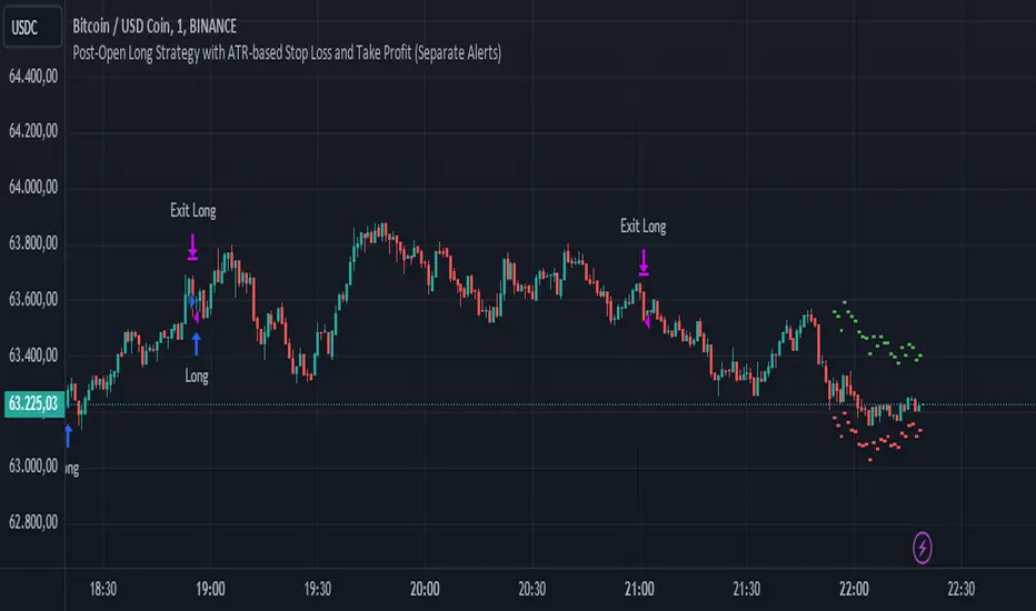
TRIN (Arms Index) Trading StrategyThe TRIN (Arms Index), also known as the Short-Term Trading Index, is a technical indicator designed to gauge the internal strength or weakness of the market. It compares the number of advancing and declining stocks to the advancing and declining volume (AD Volume). A TRIN value above 1.0 generally indicates bearish market conditions, while a value below 1.0 suggests bullish market sentiment.
Strategy Rules:
Entry Condition (Long Position): When the TRIN value is above 1.0, the strategy enters a long position, indicating that the market may be oversold, and a potential reversal could occur.
Exit Condition: The strategy exits the long position when the closing price is higher than the previous day’s high, signaling a potential rebound in the market.
This strategy aims to capitalize on short-term market inefficiencies by entering trades during periods of potential market weakness and exiting when signs of recovery appear.
How the TRIN Index Works:
The TRIN is calculated as follows:
TRIN=Advancing Issues / Declining IssuesAdvancing Volume / Declining Volume
TRIN=Advancing Volume / Declining VolumeAdvancing Issues / Declining Issues
A TRIN value above 1.0 indicates that the market is potentially oversold (more declining stocks with higher volume), while a value below 1.0 suggests the market may be overbought (more advancing stocks with higher volume) .
Empirical Evidence:
Market Sentiment Indicator: The TRIN has been widely used as a sentiment indicator. Research by Zweig (1997) suggests that extreme TRIN values can serve as a contrarian signal, indicating potential turning points in the market. For instance, a TRIN above 2.0 is often considered a sign of panic selling, which can precede a market bottom .
Overbought/Oversold Conditions: Studies have shown that indicators like TRIN, which measure market breadth and volume, can be effective in identifying overbought and oversold conditions. According to Fama and French (1988), market sentiment indicators that consider both price and volume data can offer insights into future price movements .
Risks and Limitations:
False Signals:
One of the primary risks of using the TRIN-based strategy is the possibility of false signals. A TRIN value above 1.0 does not always guarantee a market rebound, especially in sustained bearish trends. In such cases, the strategy might enter long positions prematurely, leading to losses.
Research by Brock, Lakonishok, and LeBaron (1992) found that while market indicators like TRIN can be useful, they are not foolproof and can generate multiple false positives, particularly in volatile markets .
Market Regimes:
The effectiveness of the TRIN index can vary depending on the market regime. In strongly trending markets, either bullish or bearish, the TRIN may not provide reliable reversal signals, and relying on it could result in trades that go against the prevailing trend. For instance, during strong bear markets, the TRIN may frequently remain above 1.0, leading to multiple losing trades as the market continues to decline.
Short-Term Focus:
The TRIN strategy is inherently short-term focused, aiming to capture quick market reversals. This makes it sensitive to market noise and less effective for longer-term investors. Moreover, short-term trading strategies often require more frequent adjustments and can incur higher transaction costs, which may erode profitability over time.
Liquidity and Execution Risk:
Since the TRIN strategy requires entering and exiting trades based on short-term market movements, it is vulnerable to liquidity and execution risks. In fast-moving markets, the execution of trades may be delayed, leading to slippage and potentially unfavorable entry or exit points.
Conclusion:
The TRIN (Arms Index) Trading Strategy can be an effective tool for traders looking to capitalize on short-term market inefficiencies and potential reversals. However, it is important to recognize the risks associated with this strategy, including false signals, sensitivity to market regimes, and execution risks. Traders should employ proper risk management techniques and consider combining the TRIN with other indicators to improve the robustness of the strategy.
While the TRIN provides valuable insights into market sentiment, it is not a standalone solution and should be used in conjunction with a broader trading plan that takes into account both technical and fundamental analysis.
References:
Arms, Richard W. "Volume Adjusted Moving Averages." Technical Analysis of Stocks & Commodities, 1993.
Zweig, Martin. Winning on Wall Street. Warner Books, 1997.
Fama, Eugene F., and Kenneth R. French. "Permanent and Temporary Components of Stock Prices." Journal of Political Economy, 1988.
Brock, William, Josef Lakonishok, and Blake LeBaron. "Simple Technical Trading Rules and the Stochastic Properties of Stock Returns." Journal of Finance, 1992.

Negroni Opening Range StrategyStrategy Summary:
This tool can be used to help identify breakouts from a range during a time-zone of your choosing. It plots a pre-market range, an opening range, it also includes moving average levels that can be used as confluence, as well as plotting previous day SESSION highs and lows.
There are several options on how you wish to close out the trades, all described in more detail below.
Back-testing Inputs:
You define your timezone.
You define how many trades to open on any given day.
You decide to go: long only, short only, or long & short (CAREFUL: "Long & Short" can open trades that effectively closes-out existing ones, for better AND worse!)
You define between which times the strategy will open trades.
You define when it closes any open trades (preventing overnight trades, or leaving trades open into US data times!!).
This hopefully helps make back-testing reflect YOUR trading hours.
NOTE: Renko or Heikin-Ashi charts
For ALL strategies, don’t use Renko or Heikin-Ashi charts unless you know EXACTLY the implications.
Specific to my strategy, using a renko chart can make this 85-90% profitable (I wish it was!!) Although they can be useful, renko charts don’t always capture real wicks, so the renko chart may show your trade up-only but your broker (who is not using renko!!) will have likely stopped you out on a wick somewhere along the line.
NOTE: TradingView ‘Deep backtesting’
For ALL strategies, be cynical of all backtesting (e.g. repainting issues etc) as well as ‘Deep backtesting’ results.
Specific to this strategy, the default settings here SHOULD BE OK, but unfortunately at the time of writing, we can’t see on the chart what exactly ‘deep backtesting’ is calculating. In the past I have noted a number of trades that were not closed at the end of the day, despite my ‘end of day’ trade closing being enabled, so there were big winners and losers that would not have materialized otherwise. As I say, this seems ok at these settings but just always be cynical!!
Opening Range Inputs
You define a pre-market range (example: 08:00 - 09:00).
You define an opening range (example: 09:00 - 09:30).
The strategy will give an update at the close of the opening range to let you know if the opening range has broken out the pre-market range (OR Breakout), or if it has remained inside (OR Inside). The label appears at the end of the opening range NOT at the bar that ‘broke-out’.
This is just a visual cue for you, it has no bearing on what the strategy will do.
The strategy default will trade off the pre-market range, but you can untick this if you prefer to trade off the opening range.
Opening Trades:
Strategy goes long when the bar (CLOSE) crosses-over the ‘pre-market’ high (not the ‘opening range’ high); and the time is within your trading session, and you have not maxed out your number of trades for the day!
Strategy goes short when the bar (CLOSE) crosses-under the ‘pre-market’ low (not the ‘opening range low); and the time is within your trading session, and you have not maxed out your number of trades for the day!
Remember, you can untick this if you prefer to trade off the opening range instead.
NOTES:
Using momentum indicators can help (RSI and MACD): especially to trade range plays in failed breakouts, when momentum shifts… but the strategy won’t do this for you!
Using an anchored vwap at the session open can also provide nice confluence, as well as take-profit levels at the upper/lower of 3x standard deviation.
CLOSING TRADES:
You have 6 take-profit (TP) options:
1) Full TP: uses ATR Multiplier - Full TP at the ATR parameters as defined in inputs.
2) Take Partial profits: ATR Multiplier - Takes partial profits based on parameters as defined in inputs (i.e close 40% of original trade at TP1, close another 40% of original trade at TP2, then the remainder at Full TP as set in option 1.).
3) Full TP: Trailing Stop - Applies a Trailing Stop at the number of points, as defined in inputs.
4) Full TP: MA cross - Takes profit when price crosses ‘Trend MA’ as defined in inputs.
5) Scalp: Points - closes at a set number of points, as defined in inputs.
6) Full TP: PMKT Multiplier - places a SL at opposite pre-market Hi/Low (we go long at a break-out of the pre-market high, 50% would place a SL at the pre-market range mid-point; 100% would place a SL at the pre-market low)'. This takes profit at the input set in option 1).
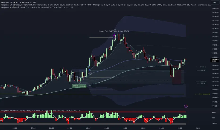
Advanced Gold Scalping Strategy with RSI Divergence# Advanced Gold Scalping Strategy with RSI Divergence
## Overview
This Pine Script implements an advanced scalping strategy for gold (XAUUSD) trading, primarily designed for the 1-minute timeframe. The strategy utilizes the Relative Strength Index (RSI) indicator along with its moving average to identify potential trade setups based on divergences between price action and RSI movements.
## Key Components
### 1. RSI Calculation
- Uses a customizable RSI length (default: 60)
- Allows selection of the source for RSI calculation (default: close price)
### 2. Moving Average of RSI
- Supports multiple MA types: SMA, EMA, SMMA (RMA), WMA, VWMA, and Bollinger Bands
- Customizable MA length (default: 3)
- Option to display Bollinger Bands with adjustable standard deviation multiplier
### 3. Divergence Detection
- Implements both bullish and bearish divergence identification
- Uses pivot high and pivot low points to detect divergences
- Allows for customization of lookback periods and range for divergence detection
### 4. Entry Conditions
- Long Entry: Bullish divergence when RSI is below 40
- Short Entry: Bearish divergence when RSI is above 60
### 5. Trade Management
- Stop Loss: Customizable, default set to 11 pips
- Take Profit: Customizable, default set to 33 pips
### 6. Visualization
- Plots RSI line and its moving average
- Displays horizontal lines at 30, 50, and 70 RSI levels
- Shows Bollinger Bands when selected
- Highlights divergences with "Bull" and "Bear" labels on the chart
## Input Parameters
- RSI Length: Adjusts the period for RSI calculation
- RSI Source: Selects the price source for RSI (close, open, high, low, hl2, hlc3, ohlc4)
- MA Type: Chooses the type of moving average applied to RSI
- MA Length: Sets the period for the moving average
- BB StdDev: Adjusts the standard deviation multiplier for Bollinger Bands
- Show Divergence: Toggles the display of divergence labels
- Stop Loss: Sets the stop loss distance in pips
- Take Profit: Sets the take profit distance in pips
## Strategy Logic
1. **RSI Calculation**:
- Computes RSI using the specified length and source
- Calculates the chosen type of moving average on the RSI
2. **Divergence Detection**:
- Identifies pivot points in both price and RSI
- Checks for higher lows in RSI with lower lows in price (bullish divergence)
- Checks for lower highs in RSI with higher highs in price (bearish divergence)
3. **Trade Entry**:
- Enters a long position when a bullish divergence is detected and RSI is below 40
- Enters a short position when a bearish divergence is detected and RSI is above 60
4. **Position Management**:
- Places a stop loss order at the entry price ± stop loss pips (depending on the direction)
- Sets a take profit order at the entry price ± take profit pips (depending on the direction)
5. **Visualization**:
- Plots the RSI and its moving average
- Draws horizontal lines for overbought/oversold levels
- Displays Bollinger Bands if selected
- Shows divergence labels on the chart for identified setups
## Usage Instructions
1. Apply the script to a 1-minute XAUUSD (Gold) chart in TradingView
2. Adjust the input parameters as needed:
- Increase RSI Length for less frequent but potentially more reliable signals
- Modify MA Type and Length to change the sensitivity of the RSI moving average
- Adjust Stop Loss and Take Profit levels based on current market volatility
3. Monitor the chart for Bull (long) and Bear (short) labels indicating potential trade setups
4. Use in conjunction with other analysis and risk management techniques
## Considerations
- This strategy is designed for short-term scalping and may not be suitable for all market conditions
- Always backtest and forward test the strategy before using it with real capital
- The effectiveness of divergence-based strategies can vary depending on market trends and volatility
- Consider using additional confirmation signals or filters to improve the strategy's performance
Remember to adapt the strategy parameters to your risk tolerance and trading style, and always practice proper risk management.
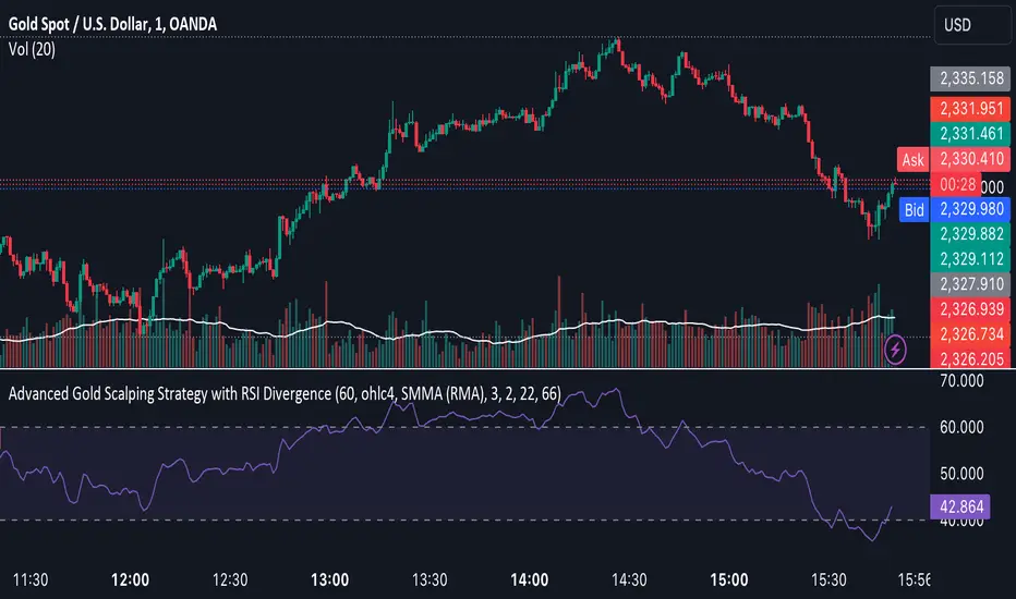
Divergent Bar Strategy [declarative] v0.2Divergent Bar Strategy v0.2
Divergent Bar is a price action that signals potential trend reversal.
This strategy uses repeating divergent bars during a bearish local trend as signals to issue multiple averaging long orders in the direction of potentially emerging bullish trend. As the local trend reverses from bearish to bullish, position could become profitable and is closed by an opposite signal.
As an averaging strategy, this strategy can accumulate substantial order sizes, so this implementation uses a stop loss which is adjusted dynamically according to the current position size to protect deposit.
What you see on a chart:
Greenish background under the divergent bars. This designates detected divergent signals.
Alligator Fast Period and Required Bar Amplitude affect the amount of divergent bars detected.
Red green and blue alligator lines display the alligator indicator used as part of divergent bar detection. In general, you don’t need to see it, you can color the lines transparent in the Style section.
Green triangles designate placed long orders. Required Divergents for Long Cummulative Signal parameter affects those signals.
Parameters and default values:
Alligator Fast Period, default 9.
Length of the alligator fast EMA. The alligator indicator used to filter a divergent bar. A bar is considered divergent only if it is located below the alligator for bollish signal and above for a bearish. In general you can leave default value, as the period 9 corresponds to a reasonable value for an alligator, used for bars on a specific timeframe.
Required Bar Amplitude (%), default 0.4.
This is an important parameter that needs to be adjusted for different timeframes. It specifies minimum size of candle shadow used to detect divergent bars. Higher values produce more false signals, lower values tend produce only strong signals. Be careful, because it also filters out bearish signals used to close the trades, so you need a bearish signal to appear. If you filter small signals you risk ending up with a trade that does not close in profit. You need to find a balance here.
Required Divergents for Long Cummulative Signal, default 3.
Divergent bar does not necessarily signal an immidiate trend reversal. Sometimes several signals need to accumulate. This parameter specifies the count at which the orders start. If you increase this count, orders are only placed after the count is achieved, so your position has bigger chance to go in profit sooner. It does not necessarily mean the most profitable position.
Required Divergents for Short Cummulative Signal, default 1.
It is the same as for long positions, but the opposite.
These signals are used to close the trades. Higher value can mean that a take profit signal would happen at potentially higher price, but be aware that it could also lead to missign oportunity to take profit if there is not enough signals in the sequence.
Long Order Size (%), default 5.0.
Percentage of deposit used for the first order in sequence. Actual order size is comuted dynamically, it depends on Reinvest and parameter. In case Reinvest is turned on, it is computed relative to the current equity, that is initial deposit and netprofit combined.
Reinvest (only for backtesting), default - turned off.
Affects Long Order Size. If turned off, order size is computed according to percentage of total equity, that is initial deposit + net profit. In an automated strategy, you should not turn this parameter on, because this way you can’t control the position size, as it growith or reduces during the actual period of the study.
Martingale, default 1.0.
Affects dynamically computed order size. First order is calculated in percentage from deposit or equity, as specified by Long Order Size and Reinvest parameters.
Order will be scaled by the following values:
Martingale = 0.0 - only the first order would be placed.
Martingale = 1.0 - equal orders will be placed in sequence, with leads to unlimited position growth.
Martingale = 1.3 - orders will be scaled by 1.3, 1.69, 2.197 etc. That is geometric increasing sequnce, which leads to unlimited position growth.
Sequential long order size is multiplied by the martingale value.
Martingale < 1.0 - orders will be scaled by geometrically decreasing sequence, resulting in limited growth of position.
Long Stop Loss (%), default 10.0.
Dynamically adjusted stop loss, which is computed according to the current average position price, so the value potentially lost is proportional to the percentage specified.
Show Long Stop Loss Line, default is off.
Draws a graph line corresponding to the dynamic stop loss on the chart.
Bullish Line Visual Offset (% of price), default -10
For convenience, the count of sequential orders is drawn as a green line over a black EMA on the same chart, offset from an EMA. This is just a visual aid to visualize the strength of long signal as divergent bars accumulate in sequence. EMA is just used so the visual cue is always displayed somewhere close the price graph.

Bitcoin 5A Strategy@LilibtcIn our long-term strategy, we have deeply explored the key factors influencing the price of Bitcoin. By precisely calculating the correlation between these factors and the price of Bitcoin, we found that they are closely linked to the value of Bitcoin. To more effectively predict the fair price of Bitcoin, we have built a predictive model and adjusted our investment strategy accordingly based on this model. In practice, the prediction results of this model correspond quite high with actual values, fully demonstrating its reliability in predicting price fluctuations.
When the future is uncertain and the outlook is unclear, people often choose to hold back and avoid risks, or even abandon their original plans. However, the prediction of Bitcoin is full of challenges, but we have taken the first step in exploring.
Table of contents:
Usage Guide
Step 1: Identify the factors that have the greatest impact on Bitcoin price
Step 2: Build a Bitcoin price prediction model
Step 3: Find indicators for warning of bear market bottoms and bull market tops
Step 4: Predict Bitcoin Price in 2025
Step 5: Develop a Bitcoin 5A strategy
Step 6: Verify the performance of the Bitcoin 5A strategy
Usage Restrictions
🦮Usage Guide:
1. On the main interface, modify the code, find the BTCUSD trading pair, and select the BITSTAMP exchange for trading.
2. Set the time period to the daily chart.
3. Select a logarithmic chart in the chart type to better identify price trends.
4. In the strategy settings, adjust the options according to personal needs, including language, display indicators, display strategies, display performance, display optimizations, sell alerts, buy prompts, opening days, backtesting start year, backtesting start month, and backtesting start date.
🏃Step 1: Identify the factors that have the greatest impact on Bitcoin price
📖Correlation Coefficient: A mathematical concept for measuring influence
In order to predict the price trend of Bitcoin, we need to delve into the factors that have the greatest impact on its price. These factors or variables can be expressed in mathematical or statistical correlation coefficients. The correlation coefficient is an indicator of the degree of association between two variables, ranging from -1 to 1. A value of 1 indicates a perfect positive correlation, while a value of -1 indicates a perfect negative correlation.
For example, if the price of corn rises, the price of live pigs usually rises accordingly, because corn is the main feed source for pig breeding. In this case, the correlation coefficient between corn and live pig prices is approximately 0.3. This means that corn is a factor affecting the price of live pigs. On the other hand, if a shooter's performance improves while another shooter's performance deteriorates due to increased psychological pressure, we can say that the former is a factor affecting the latter's performance.
Therefore, in order to identify the factors that have the greatest impact on the price of Bitcoin, we need to find the factors with the highest correlation coefficients with the price of Bitcoin. If, through the analysis of the correlation between the price of Bitcoin and the data on the chain, we find that a certain data factor on the chain has the highest correlation coefficient with the price of Bitcoin, then this data factor on the chain can be identified as the factor that has the greatest impact on the price of Bitcoin. Through calculation, we found that the 🔵number of Bitcoin blocks is one of the factors that has the greatest impact on the price of Bitcoin. From historical data, it can be clearly seen that the growth rate of the 🔵number of Bitcoin blocks is basically consistent with the movement direction of the price of Bitcoin. By analyzing the past ten years of data, we obtained a daily correlation coefficient of 0.93 between the number of Bitcoin blocks and the price of Bitcoin.
🏃Step 2: Build a Bitcoin price prediction model
📖Predictive Model: What formula is used to predict the price of Bitcoin?
Among various prediction models, the linear function is the preferred model due to its high accuracy. Take the standard weight as an example, its linear function graph is a straight line, which is why we choose the linear function model. However, the growth rate of the price of Bitcoin and the number of blocks is extremely fast, which does not conform to the characteristics of the linear function. Therefore, in order to make them more in line with the characteristics of the linear function, we first take the logarithm of both. By observing the logarithmic graph of the price of Bitcoin and the number of blocks, we can find that after the logarithm transformation, the two are more in line with the characteristics of the linear function. Based on this feature, we choose the linear regression model to establish the prediction model.
From the graph below, we can see that the actual red and green K-line fluctuates around the predicted blue and 🟢green line. These predicted values are based on fundamental factors of Bitcoin, which support its value and reflect its reasonable value. This picture is consistent with the theory proposed by Marx in "Das Kapital" that "prices fluctuate around values."
The predicted logarithm of the market cap of Bitcoin is calculated through the model. The specific calculation formula of the Bitcoin price prediction value is as follows:
btc_predicted_marketcap = math.exp(btc_predicted_marketcap_log)
btc_predicted_price = btc_predicted_marketcap / btc_supply
🏃Step 3: Find indicators for early warning of bear market bottoms and bull market tops
📖Warning Indicator: How to Determine Whether the Bitcoin Price has Reached the Bear Market Bottom or the Bull Market Top?
By observing the Bitcoin price logarithmic prediction chart mentioned above, we notice that the actual price often falls below the predicted value at the bottom of a bear market; during the peak of a bull market, the actual price exceeds the predicted price. This pattern indicates that the deviation between the actual price and the predicted price can serve as an early warning signal. When the 🔴 Bitcoin price deviation is very low, as shown by the chart with 🟩green background, it usually means that we are at the bottom of the bear market; Conversely, when the 🔴 Bitcoin price deviation is very high, the chart with a 🟥red background indicates that we are at the peak of the bull market.
This pattern has been validated through six bull and bear markets, and the deviation value indeed serves as an early warning signal, which can be used as an important reference for us to judge market trends.
🏃Step 4:Predict Bitcoin Price in 2025
📖Price Upper Limit
According to the data calculated on February 25, 2024, the 🟠upper limit of the Bitcoin price is $194,287, which is the price ceiling of this bull market. The peak of the last bull market was on November 9, 2021, at $68,664. The bull-bear market cycle is 4 years, so the highest point of this bull market is expected in 2025. That is where you should sell the Bitcoin. and the upper limit of the Bitcoin price will exceed $190,000. The closing price of Bitcoin on February 25, 2024, was $51,729, with an expected increase of 2.7 times.
🏃Step 5: Bitcoin 5A Strategy Formulation
📖Strategy: When to buy or sell, and how many to choose?
We introduce the Bitcoin 5A strategy. This strategy requires us to generate trading signals based on the critical values of the warning indicators, simulate the trades, and collect performance data for evaluation. In the Bitcoin 5A strategy, there are three key parameters: buying warning indicator, batch trading days, and selling warning indicator. Batch trading days are set to ensure that we can make purchases in batches after the trading signal is sent, thus buying at a lower price, selling at a higher price, and reducing the trading impact cost.
In order to find the optimal warning indicator critical value and batch trading days, we need to adjust these parameters repeatedly and perform backtesting. Backtesting is a method established by observing historical data, which can help us better understand market trends and trading opportunities.
Specifically, we can find the key trading points by watching the Bitcoin price log and the Bitcoin price deviation chart. For example, on August 25, 2015, the 🔴 Bitcoin price deviation was at its lowest value of -1.11; on December 17, 2017, the 🔴 Bitcoin price deviation was at its highest value at the time, 1.69; on March 16, 2020, the 🔴 Bitcoin price deviation was at its lowest value at the time, -0.91; on March 13, 2021, the 🔴 Bitcoin price deviation was at its highest value at the time, 1.1; on December 31, 2022, the 🔴 Bitcoin price deviation was at its lowest value at the time, -1.
To ensure that all five key trading points generate trading signals, we set the warning indicator Bitcoin price deviation to the larger of the three lowest values, -0.9, and the smallest of the two highest values, 1. Then, we buy when the warning indicator Bitcoin price deviation is below -0.9, and sell when it is above 1.
In addition, we set the batch trading days as 25 days to implement a strategy that averages purchases and sales. Within these 25 days, we will invest all funds into the market evenly, buying once a day. At the same time, we also sell positions at the same pace, selling once a day.
📖Adjusting the threshold: a key step to optimizing trading strategy
Adjusting the threshold is an indispensable step for better performance. Here are some suggestions for adjusting the batch trading days and critical values of warning indicators:
• Batch trading days: Try different days like 25 to see how it affects overall performance.
• Buy and sell critical values for warning indicators: iteratively fine-tune the buy threshold value of -0.9 and the sell threshold value of 1 exhaustively to find the best combination of threshold values.
Through such careful adjustments, we may find an optimized approach with a lower maximum drawdown rate (e.g., 11%) and a higher cumulative return rate for closed trades (e.g., 474 times). The chart below is a backtest optimization chart for the Bitcoin 5A strategy, providing an intuitive display of strategy adjustments and optimizations.
In this way, we can better grasp market trends and trading opportunities, thereby achieving a more robust and efficient trading strategy.
🏃Step 6: Validating the performance of the Bitcoin 5A Strategy
📖Model interpretability validation: How to explain the Bitcoin price model?
The interpretability of the model is represented by the coefficient of determination R squared, which reflects the degree of match between the predicted value and the actual value. I divided all the historical data from August 18, 2015 into two groups, and used the data from August 18, 2011 to August 18, 2015 as training data to generate the model. The calculation result shows that the coefficient of determination R squared during the 2011-2015 training period is as high as 0.81, which shows that the interpretability of this model is quite high. From the Bitcoin price logarithmic prediction chart in the figure below, we can see that the deviation between the predicted value and the actual value is not far, which means that most of the predicted values can explain the actual value well.
The calculation formula for the coefficient of determination R squared is as follows:
residual = btc_close_log - btc_predicted_price_log
residual_square = residual * residual
train_residual_square_sum = math.sum(residual_square, train_days)
train_mse = train_residual_square_sum / train_days
train_r2 = 1 - train_mse / ta.variance(btc_close_log, train_days)
📖Model stability verification: How to affirm the stability of the Bitcoin price model when new data is available?
Model stability is achieved through model verification. I set the last day of the training period to February 2, 2024 as the "verification group" and used it as verification data to verify the stability of the model. This means that after generating the model if there is new data, I will use these new data together with the model for prediction, and then evaluate the interpretability of the model. If the coefficient of determination when using verification data is close to the previous training one and both remain at a high level, then we can consider this model as stability. The coefficient of determination calculated from the validation period data and model prediction results is as high as 0.83, which is close to the previous 0.81, further proving the stability of this model.
📖Performance evaluation: How to accurately evaluate historical backtesting results?
After detailed strategy testing, to ensure the accuracy and reliability of the results, we need to carry out a detailed performance evaluation on the backtest results. The key evaluation indices include:
• Net value curve: As shown in the rose line, it intuitively reflects the growth of the account net value. By observing the net value curve, we can understand the overall performance and profitability of the strategy.
The basic attributes of this strategy are as follows:
Trading range: 2015-8-19 to 2024-2-18, backtest range: 2011-8-18 to 2024-2-18
Initial capital: 1000USD, order size: 1 contract, pyramid: 50 orders, commission rate: 0.2%, slippage: 20 markers.
In the strategy tester overview chart, we also obtained the following key data:
• Net profit rate of closed trades: as high as 474 times, far exceeding the benchmark, as shown in the strategy tester performance summary chart, Bitcoin buys and holds 210 times.
• Number of closed trades and winning percentage: 100 trades were all profitable, showing the stability and reliability of the strategy.
• Drawdown rate & win-loose ratio: The maximum drawdown rate is only 11%, far lower than Bitcoin's 78%. Profit factor, or win-loose ratio, reached 500, further proving the advantage of the strategy.
Through these detailed evaluations, we can see clearly the excellent balance between risk and return of the Bitcoin 5A strategy.
⚠️Usage Restrictions: Strategy Application in Specific Situations
Please note that this strategy is designed specifically for Bitcoin and should not be applied to other assets or markets without authorization. In actual operations, we should make careful decisions according to our risk tolerance and investment goals.

Bitcoin 5A Strategy - Price Upper & Lower Limit@LilibtcIn our long-term strategy, we have deeply explored the key factors influencing the price of Bitcoin. By precisely calculating the correlation between these factors and the price of Bitcoin, we found that they are closely linked to the value of Bitcoin. To more effectively predict the fair price of Bitcoin, we have built a predictive model and adjusted our investment strategy accordingly based on this model. In practice, the prediction results of this model correspond quite high with actual values, fully demonstrating its reliability in predicting price fluctuations.
When the future is uncertain and the outlook is unclear, people often choose to hold back and avoid risks, or even abandon their original plans. However, the prediction of Bitcoin is full of challenges, but we have taken the first step in exploring.
Table of contents:
Usage Guide
Step 1: Identify the factors that have the greatest impact on Bitcoin price
Step 2: Build a Bitcoin price prediction model
Step 3: Find indicators for warning of bear market bottoms and bull market tops
Step 4: Predict Bitcoin Price in 2025
Step 5: Develop a Bitcoin 5A strategy
Step 6: Verify the performance of the Bitcoin 5A strategy
Usage Restrictions
🦮Usage Guide:
1. On the main interface, modify the code, find the BTCUSD trading pair, and select the BITSTAMP exchange for trading.
2. Set the time period to the daily chart.
3. Select a logarithmic chart in the chart type to better identify price trends.
4. In the strategy settings, adjust the options according to personal needs, including language, display indicators, display strategies, display performance, display optimizations, sell alerts, buy prompts, opening days, backtesting start year, backtesting start month, and backtesting start date.
🏃Step 1: Identify the factors that have the greatest impact on Bitcoin price
📖Correlation Coefficient: A mathematical concept for measuring influence
In order to predict the price trend of Bitcoin, we need to delve into the factors that have the greatest impact on its price. These factors or variables can be expressed in mathematical or statistical correlation coefficients. The correlation coefficient is an indicator of the degree of association between two variables, ranging from -1 to 1. A value of 1 indicates a perfect positive correlation, while a value of -1 indicates a perfect negative correlation.
For example, if the price of corn rises, the price of live pigs usually rises accordingly, because corn is the main feed source for pig breeding. In this case, the correlation coefficient between corn and live pig prices is approximately 0.3. This means that corn is a factor affecting the price of live pigs. On the other hand, if a shooter's performance improves while another shooter's performance deteriorates due to increased psychological pressure, we can say that the former is a factor affecting the latter's performance.
Therefore, in order to identify the factors that have the greatest impact on the price of Bitcoin, we need to find the factors with the highest correlation coefficients with the price of Bitcoin. If, through the analysis of the correlation between the price of Bitcoin and the data on the chain, we find that a certain data factor on the chain has the highest correlation coefficient with the price of Bitcoin, then this data factor on the chain can be identified as the factor that has the greatest impact on the price of Bitcoin. Through calculation, we found that the 🔵 number of Bitcoin blocks is one of the factors that has the greatest impact on the price of Bitcoin. From historical data, it can be clearly seen that the growth rate of the 🔵 number of Bitcoin blocks is basically consistent with the movement direction of the price of Bitcoin. By analyzing the past ten years of data, we obtained a daily correlation coefficient of 0.93 between the number of Bitcoin blocks and the price of Bitcoin.
🏃Step 2: Build a Bitcoin price prediction model
📖Predictive Model: What formula is used to predict the price of Bitcoin?
Among various prediction models, the linear function is the preferred model due to its high accuracy. Take the standard weight as an example, its linear function graph is a straight line, which is why we choose the linear function model. However, the growth rate of the price of Bitcoin and the number of blocks is extremely fast, which does not conform to the characteristics of the linear function. Therefore, in order to make them more in line with the characteristics of the linear function, we first take the logarithm of both. By observing the logarithmic graph of the price of Bitcoin and the number of blocks, we can find that after the logarithm transformation, the two are more in line with the characteristics of the linear function. Based on this feature, we choose the linear regression model to establish the prediction model.
From the graph below, we can see that the actual red and green K-line fluctuates around the predicted blue and 🟢green line. These predicted values are based on fundamental factors of Bitcoin, which support its value and reflect its reasonable value. This picture is consistent with the theory proposed by Marx in "Das Kapital" that "prices fluctuate around values."
The predicted logarithm of the market cap of Bitcoin is calculated through the model. The specific calculation formula of the Bitcoin price prediction value is as follows:
btc_predicted_marketcap = math.exp(btc_predicted_marketcap_log)
btc_predicted_price = btc_predicted_marketcap / btc_supply
🏃Step 3: Find indicators for early warning of bear market bottoms and bull market tops
📖Warning Indicator: How to Determine Whether the Bitcoin Price has Reached the Bear Market Bottom or the Bull Market Top?
By observing the Bitcoin price logarithmic prediction chart mentioned above, we notice that the actual price often falls below the predicted value at the bottom of a bear market; during the peak of a bull market, the actual price exceeds the predicted price. This pattern indicates that the deviation between the actual price and the predicted price can serve as an early warning signal. When the 🔴 Bitcoin price deviation is very low, as shown by the chart with 🟩green background, it usually means that we are at the bottom of the bear market; Conversely, when the 🔴 Bitcoin price deviation is very high, the chart with a 🟥red background indicates that we are at the peak of the bull market.
This pattern has been validated through six bull and bear markets, and the deviation value indeed serves as an early warning signal, which can be used as an important reference for us to judge market trends.
🏃Step 4:Predict Bitcoin Price in 2025
📖Price Upper Limit
According to the data calculated on March 10, 2023(If you want to check latest data, please contact with author), the 🟠upper limit of the Bitcoin price is $132,453, which is the price ceiling of this bull market. The peak of the last bull market was on November 9, 2021, at $68,664. The bull-bear market cycle is 4 years, so the highest point of this bull market is expected in 2025, and the 🟠upper limit of the Bitcoin price will exceed $130,000. The closing price of Bitcoin on March 10, 2024, was $68,515, with an expected increase of 90%.
🏃Step 5: Bitcoin 5A Strategy Formulation
📖Strategy: When to buy or sell, and how many to choose?
We introduce the Bitcoin 5A strategy. This strategy requires us to generate trading signals based on the critical values of the warning indicators, simulate the trades, and collect performance data for evaluation. In the Bitcoin 5A strategy, there are three key parameters: buying warning indicator, batch trading days, and selling warning indicator. Batch trading days are set to ensure that we can make purchases in batches after the trading signal is sent, thus buying at a lower price, selling at a higher price, and reducing the trading impact cost.
In order to find the optimal warning indicator critical value and batch trading days, we need to adjust these parameters repeatedly and perform backtesting. Backtesting is a method established by observing historical data, which can help us better understand market trends and trading opportunities.
Specifically, we can find the key trading points by watching the Bitcoin price log and the Bitcoin price deviation chart. For example, on August 25, 2015, the 🔴 Bitcoin price deviation was at its lowest value of -1.11; on December 17, 2017, the 🔴 Bitcoin price deviation was at its highest value at the time, 1.69; on March 16, 2020, the 🔴 Bitcoin price deviation was at its lowest value at the time, -0.91; on March 13, 2021, the 🔴 Bitcoin price deviation was at its highest value at the time, 1.1; on December 31, 2022, the 🔴 Bitcoin price deviation was at its lowest value at the time, -1.
To ensure that all five key trading points generate trading signals, we set the warning indicator Bitcoin price deviation to the larger of the three lowest values, -0.9, and the smallest of the two highest values, 1. Then, we buy when the warning indicator Bitcoin price deviation is below -0.9, and sell when it is above 1.
In addition, we set the batch trading days as 25 days to implement a strategy that averages purchases and sales. Within these 25 days, we will invest all funds into the market evenly, buying once a day. At the same time, we also sell positions at the same pace, selling once a day.
📖Adjusting the threshold: a key step to optimizing trading strategy
Adjusting the threshold is an indispensable step for better performance. Here are some suggestions for adjusting the batch trading days and critical values of warning indicators:
• Batch trading days: Try different days like 25 to see how it affects overall performance.
• Buy and sell critical values for warning indicators: iteratively fine-tune the buy threshold value of -0.9 and the sell threshold value of 1 exhaustively to find the best combination of threshold values.
Through such careful adjustments, we may find an optimized approach with a lower maximum drawdown rate (e.g., 11%) and a higher cumulative return rate for closed trades (e.g., 474 times). The chart below is a backtest optimization chart for the Bitcoin 5A strategy, providing an intuitive display of strategy adjustments and optimizations.
In this way, we can better grasp market trends and trading opportunities, thereby achieving a more robust and efficient trading strategy.
🏃Step 6: Validating the performance of the Bitcoin 5A Strategy
📖Model accuracy validation: How to judge the accuracy of the Bitcoin price model?
The accuracy of the model is represented by the coefficient of determination R square, which reflects the degree of match between the predicted value and the actual value. I divided all the historical data from August 18, 2015 into two groups, and used the data from August 18, 2011 to August 18, 2015 as training data to generate the model. The calculation result shows that the coefficient of determination R squared during the 2011-2015 training period is as high as 0.81, which shows that the accuracy of this model is quite high. From the Bitcoin price logarithmic prediction chart in the figure below, we can see that the deviation between the predicted value and the actual value is not far, which means that most of the predicted values can explain the actual value well.
The calculation formula for the coefficient of determination R square is as follows:
residual = btc_close_log - btc_predicted_price_log
residual_square = residual * residual
train_residual_square_sum = math.sum(residual_square, train_days)
train_mse = train_residual_square_sum / train_days
train_r2 = 1 - train_mse / ta.variance(btc_close_log, train_days)
📖Model reliability verification: How to affirm the reliability of the Bitcoin price model when new data is available?
Model reliability is achieved through model verification. I set the last day of the training period to February 2, 2024 as the "verification group" and used it as verification data to verify the reliability of the model. This means that after generating the model if there is new data, I will use these new data together with the model for prediction, and then evaluate the accuracy of the model. If the coefficient of determination when using verification data is close to the previous training one and both remain at a high level, then we can consider this model as reliable. The coefficient of determination calculated from the validation period data and model prediction results is as high as 0.83, which is close to the previous 0.81, further proving the reliability of this model.
📖Performance evaluation: How to accurately evaluate historical backtesting results?
After detailed strategy testing, to ensure the accuracy and reliability of the results, we need to carry out a detailed performance evaluation on the backtest results. The key evaluation indices include:
• Net value curve: As shown in the rose line, it intuitively reflects the growth of the account net value. By observing the net value curve, we can understand the overall performance and profitability of the strategy.
The basic attributes of this strategy are as follows:
Trading range: 2015-8-19 to 2024-2-18, backtest range: 2011-8-18 to 2024-2-18
Initial capital: 1000USD, order size: 1 contract, pyramid: 50 orders, commission rate: 0.2%, slippage: 20 markers.
In the strategy tester overview chart, we also obtained the following key data:
• Net profit rate of closed trades: as high as 474 times, far exceeding the benchmark, as shown in the strategy tester performance summary chart, Bitcoin buys and holds 210 times.
• Number of closed trades and winning percentage: 100 trades were all profitable, showing the stability and reliability of the strategy.
• Drawdown rate & win-loose ratio: The maximum drawdown rate is only 11%, far lower than Bitcoin's 78%. Profit factor, or win-loose ratio, reached 500, further proving the advantage of the strategy.
Through these detailed evaluations, we can see clearly the excellent balance between risk and return of the Bitcoin 5A strategy.
⚠️Usage Restrictions: Strategy Application in Specific Situations
Please note that this strategy is designed specifically for Bitcoin and should not be applied to other assets or markets without authorization. In actual operations, we should make careful decisions according to our risk tolerance and investment goals.

Bitcoin Momentum StrategyThis is a very simple long-only strategy I've used since December 2022 to manage my Bitcoin position.
I'm sharing it as an open-source script for other traders to learn from the code and adapt it to their liking if they find the system concept interesting.
General Overview
Always do your own research and backtesting - this script is not intended to be traded blindly (no script should be) and I've done limited testing on other markets beyond Ethereum and BTC, it's just a template to tweak and play with and make into one's own.
The results shown in the strategy tester are from Bitcoin's inception so as to get a large sample size of trades, and potential returns have diminished significantly as BTC has grown to become a mega cap asset, but the script includes a date filter for backtesting and it has still performed solidly in recent years (speaking from personal experience using it myself - DYOR with the date filter).
The main advantage of this system in my opinion is in limiting the max drawdown significantly versus buy & hodl. Theoretically much better returns can be made by just holding, but that's also a good way to lose 70%+ of your capital in the inevitable bear markets (also speaking from experience).
In saying all of that, the future is fundamentally unknowable and past results in no way guarantee future performance.
System Concept:
Capture as much Bitcoin upside volatility as possible while side-stepping downside volatility as quickly as possible.
The system uses a simple but clever momentum-style trailing stop technique I learned from one of my trading mentors who uses this approach on momentum/trend-following stock market systems.
Basically, the system "ratchets" up the stop-loss to be much tighter during high bearish volatility to protect open profits from downside moves, but loosens the stop loss during sustained bullish momentum to let the position ride.
It is invested most of the time, unless BTC is trading below its 20-week EMA in which case it stays in cash/USDT to avoid holding through bear markets. It only trades one position (no pyramiding) and does not trade short, but can easily be tweaked to do whatever you like if you know what you're doing in Pine.
Default parameters:
HTF: Weekly Chart
EMA: 20-Period
ATR: 5-period
Bar Lookback: 7
Entry Rule #1:
Bitcoin's current price must be trading above its higher-timeframe EMA (Weekly 20 EMA).
Entry Rule #2:
Bitcoin must not be in 'caution' condition (no large bearish volatility swings recently).
Enter at next bar's open if conditions are met and we are not already involved in a trade.
"Caution" Condition:
Defined as true if BTC's recent 7-bar swing high minus current bar's low is > 1.5x ATR, or Daily close < Daily 20-EMA.
Trailing Stop:
Stop is trailed 1 ATR from recent swing high, or 20% of ATR if in caution condition (ie. 0.2 ATR).
Exit on next bar open upon a close below stop loss.
I typically use a limit order to open & exit trades as close to the open price as possible to reduce slippage, but the strategy script uses market orders.
I've never had any issues getting filled on limit orders close to the market price with BTC on the Daily timeframe, but if the exchange has relatively low slippage I've found market orders work fine too without much impact on the results particularly since BTC has consistently remained above $20k and highly liquid.
Cost of Trading:
The script uses no leverage and a default total round-trip commission of 0.3% which is what I pay on my exchange based on their tier structure, but this can vary widely from exchange to exchange and higher commission fees will have a significantly negative impact on realized gains so make sure to always input the correct theoretical commission cost when backtesting any script.
Static slippage is difficult to estimate in the strategy tester given the wide range of prices & liquidity BTC has experienced over the years and it largely depends on position size, I set it to 150 points per buy or sell as BTC is currently very liquid on the exchange I trade and I use limit orders where possible to enter/exit positions as close as possible to the market's open price as it significantly limits my slippage.
But again, this can vary a lot from exchange to exchange (for better or worse) and if BTC volatility is high at the time of execution this can have a negative impact on slippage and therefore real performance, so make sure to adjust it according to your exchange's tendencies.
Tax considerations should also be made based on short-term trade frequency if crypto profits are treated as a CGT event in your region.
Summary:
A simple, but effective and fairly robust system that achieves the goals I set for it.
From my preliminary testing it appears it may also work on altcoins but it might need a bit of tweaking/loosening with the trailing stop distance as the default parameters are designed to work with Bitcoin which obviously behaves very differently to smaller cap assets.
Good luck out there!
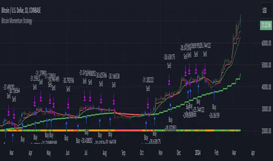
BigBeluga - BacktestingThe Backtesting System (SMC) is a strategy builder designed around concepts of Smart Money.
What makes this indicator unique is that users can build a wide variety of strategies thanks to the external source conditions and the built-in one that are coded around concepts of smart money.
🔶 FEATURES
🔹 Step Algorithm
Crafting Your Strategy:
You can add multiple steps to your strategy, using both internal and external (custom) conditions.
Evaluating Your Conditions:
The system evaluates your conditions sequentially.
Only after the previous step becomes true will the next one be evaluated.
This ensures your strategy only triggers when all specified conditions are met.
Executing Your Strategy:
Once all steps in your strategy are true, the backtester automatically opens a market order.
You can also configure exit conditions within the strategy builder to manage your positions effectively.
🔹 External and Internal build-in conditions
Users can choose to use external or internal conditions or just one of the two categories.
Build-in conditions:
CHoCH or BOS
CHoCH or BOS Sweep
CHoCH
BOS
CHoCH Sweep
BOS Sweep
OB Mitigated
Price Inside OB
FVG Mitigated
Raid Found
Price Inside FVG
SFP Created
Liquidity Print
Sweep Area
Breakdown of each of the options:
CHoCH: Change of Character (not Charter) is a change from bullish to bearish market or vice versa.
BOS: Break of Structure is a continuation of the current trend.
CHoCH or BOS Sweep: Liquidity taken out from the market within the structure.
OB Mitigated: An order block mitigated.
FVG Mitigated: An imbalance mitigated.
Raid Found: Liquidity taken out from an imbalance.
SFP Created: A Swing Failure Pattern detected.
Liquidity Print: A huge chunk of liquidity taken out from the market.
Sweep Area: A level regained from the structure.
Price inside OB/FVG: Price inside an order block or an imbalance.
External inputs can be anything that is plotted on the chart that has valid entry points, such as an RSI or a simple Supertrend.
Equal
Greather Than
Less Than
Crossing Over
Crossing Under
Crossing
🔹 Direction
Users can change the direction of each condition to either Bullish or Bearish. This can be useful if users want to long the market on a bearish condition or vice versa.
🔹 Build-in Stop-Loss and Take-Profit features
Tailoring Your Exits:
Similar to entry creation, the backtesting system allows you to build multi-step exit strategies.
Each step can utilize internal and external (custom) conditions.
This flexibility allows you to personalize your exit strategy based on your risk tolerance and trading goals.
Stop-Loss and Take-Profit Options:
The backtesting system offers various options for setting stop-loss and take-profit levels.
You can choose from:
Dynamic levels: These levels automatically adjust based on market movements, helping you manage risk and secure profits.
Specific price levels: You can set fixed stop-loss and take-profit levels based on your comfort level and analysis.
Price - Set x point to a specific price
Currency - Set x point away from tot Currency points
Ticks - Set x point away from tot ticks
Percent - Set x point away from a fixed %
ATR - Set x point away using the Averge True Range (200 bars)
Trailing Stop (Only for stop-loss order)
🔶 USAGE
Users can create a variety of strategies using this script, limited only by their imagination.
Long entry : Bullish CHoCH after price is inside a bullish order block
Short entry : Bearish CHoCH after price is inside a bearish order block
Stop-Loss : Trailing Stop set away from price by 0.2%
Example below using external conditions
Long entry : Bullish Liquidity Prints after bullish CHoCH
Short entry : Bearish Liquidity Prints after Bearish CHoCH
Long Exit : RSI Crossing over 70 line
Short Exit : RSI Crossing over 30 line
Stop-Loss : Trailing Stop set away from price by 0.3%
🔶 PROPERTIES
Users will need to adjust the property tabs according to their individual balance to achieve realistic results.
An important aspect to note is that past performance does not guarantee future results. This principle should always be kept in mind.
🔶 HOW TO ACCESS
You can see the Author Instructions to get access.
Bezahltes Script

AI SuperTrend x Pivot Percentile - Strategy [PresentTrading]█ Introduction and How it is Different
The AI SuperTrend x Pivot Percentile strategy is a sophisticated trading approach that integrates AI-driven analysis with traditional technical indicators. Combining the AI SuperTrend with the Pivot Percentile strategy highlights several key advantages:
1. Enhanced Accuracy in Trend Prediction: The AI SuperTrend utilizes K-Nearest Neighbors (KNN) algorithm for trend prediction, improving accuracy by considering historical data patterns. This is complemented by the Pivot Percentile analysis which provides additional context on trend strength.
2. Comprehensive Market Analysis: The integration offers a multi-faceted approach to market analysis, combining AI insights with traditional technical indicators. This dual approach captures a broader range of market dynamics.
BTC 6H L/S Performance
Local
█ Strategy: How it Works - Detailed Explanation
🔶 AI-Enhanced SuperTrend Indicators
1. SuperTrend Calculation:
- The SuperTrend indicator is calculated using a moving average and the Average True Range (ATR). The basic formula is:
- Upper Band = Moving Average + (Multiplier × ATR)
- Lower Band = Moving Average - (Multiplier × ATR)
- The moving average type (SMA, EMA, WMA, RMA, VWMA) and the length of the moving average and ATR are adjustable parameters.
- The direction of the trend is determined based on the position of the closing price in relation to these bands.
2. AI Integration with K-Nearest Neighbors (KNN):
- The KNN algorithm is applied to predict trend direction. It uses historical price data and SuperTrend values to classify the current trend as bullish or bearish.
- The algorithm calculates the 'distance' between the current data point and historical points. The 'k' nearest data points (neighbors) are identified based on this distance.
- A weighted average of these neighbors' trends (bullish or bearish) is calculated to predict the current trend.
For more please check: Multi-TF AI SuperTrend with ADX - Strategy
🔶 Pivot Percentile Analysis
1. Percentile Calculation:
- This involves calculating the percentile ranks for high and low prices over a set of predefined lengths.
- The percentile function is typically defined as:
- Percentile = Value at (P/100) × (N + 1)th position
- Where P is the desired percentile, and N is the number of data points.
2. Trend Strength Evaluation:
- The calculated percentiles for highs and lows are used to determine the strength of bullish and bearish trends.
- For instance, a high percentile rank in the high prices may indicate a strong bullish trend, and vice versa for bearish trends.
For more please check: Pivot Percentile Trend - Strategy
🔶 Strategy Integration
1. Combining SuperTrend and Pivot Percentile:
- The strategy synthesizes the insights from both AI-enhanced SuperTrend and Pivot Percentile analysis.
- It compares the trend direction indicated by the SuperTrend with the strength of the trend as suggested by the Pivot Percentile analysis.
2. Signal Generation:
- A trading signal is generated when both the AI-enhanced SuperTrend and the Pivot Percentile analysis agree on the trend direction.
- For instance, a bullish signal is generated when both the SuperTrend is bullish, and the Pivot Percentile analysis shows strength in bullish trends.
🔶 Risk Management and Filters
- ADX and DMI Filter: The strategy uses the Average Directional Index (ADX) and the Directional Movement Index (DMI) as filters to assess the trend's strength and direction.
- Dynamic Trailing Stop Loss: Based on the SuperTrend indicator, the strategy dynamically adjusts stop-loss levels to manage risk effectively.
This strategy stands out for its ability to combine real-time AI analysis with established technical indicators, offering traders a nuanced and responsive tool for navigating complex market conditions. The equations and algorithms involved are pivotal in accurately identifying market trends and potential trade opportunities.
█ Usage
To effectively use this strategy, traders should:
1. Understand the AI and Pivot Percentile Indicators: A clear grasp of how these indicators work will enable traders to make informed decisions.
2. Interpret the Signals Accurately: The strategy provides bullish, bearish, and neutral signals. Traders should align these signals with their market analysis and trading goals.
3. Monitor Market Conditions: Given that this strategy is sensitive to market dynamics, continuous monitoring is crucial for timely decision-making.
4. Adjust Settings as Needed: Traders should feel free to tweak the input parameters to suit their trading preferences and to respond to changing market conditions.
█Default Settings and Their Impact on Performance
1. Trading Direction (Default: "Both")
Effect: Determines whether the strategy will take long positions, short positions, or both. Adjusting this setting can align the strategy with the trader's market outlook or risk preference.
2. AI Settings (Neighbors: 3, Data Points: 24)
Neighbors: The number of nearest neighbors in the KNN algorithm. A higher number might smooth out noise but could miss subtle, recent changes. A lower number makes the model more sensitive to recent data but may increase noise.
Data Points: Defines the amount of historical data considered. More data points provide a broader context but may dilute recent trends' impact.
3. SuperTrend Settings (Length: 10, Factor: 3.0, MA Source: "WMA")
Length: Affects the sensitivity of the SuperTrend indicator. A longer length results in a smoother, less sensitive indicator, ideal for long-term trends.
Factor: Determines the bandwidth of the SuperTrend. A higher factor creates wider bands, capturing larger price movements but potentially missing short-term signals.
MA Source: The type of moving average used (e.g., WMA - Weighted Moving Average). Different MA types can affect the trend indicator's responsiveness and smoothness.
4. AI Trend Prediction Settings (Price Trend: 10, Prediction Trend: 80)
Price Trend and Prediction Trend Lengths: These settings define the lengths of weighted moving averages for price and SuperTrend, impacting the responsiveness and smoothness of the AI's trend predictions.
5. Pivot Percentile Settings (Length: 10)
Length: Influences the calculation of pivot percentiles. A shorter length makes the percentile more responsive to recent price changes, while a longer length offers a broader view of price trends.
6. ADX and DMI Settings (ADX Length: 14, Time Frame: 'D')
ADX Length: Defines the period for the Average Directional Index calculation. A longer period results in a smoother ADX line.
Time Frame: Sets the time frame for the ADX and DMI calculations, affecting the sensitivity to market changes.
7. Commission, Slippage, and Initial Capital
These settings relate to transaction costs and initial investment, directly impacting net profitability and strategy feasibility.

Pivot Percentile Trend - Strategy [presentTrading]
█ Introduction and How it is Different
The "Pivot Percentile Trend - Strategy" from PresentTrading represents a paradigm shift in technical trading strategies. What sets this strategy apart is its innovative use of pivot percentiles, a method that goes beyond traditional indicator-based analyses. Unlike standard strategies that might depend on single-dimensional signals, this approach takes a multi-layered view of market movements, blending percentile calculations with SuperTrend indicators for a more nuanced and dynamic market analysis.
This strategy stands out for its ability to process multiple data points across various timeframes and pivot lengths, thereby capturing a broader and more detailed picture of market trends. It's not just about following the price; it's about understanding its position in the context of recent historical highs and lows, offering a more profound insight into potential market movements.
BTC 6h L/S
Where traditional methods might react to market changes, the Pivot Percentile Trend strategy anticipates them, using a calculated approach to identify trend strengths and weaknesses. This foresight gives traders a significant advantage, allowing for more strategic decision-making and potentially increasing the chances of successful trades.
In essence, this strategy introduces a more comprehensive and proactive approach to trading, harnessing the power of advanced percentile calculations combined with the robustness of SuperTrend indicators. It's a strategy designed for traders who seek a deeper understanding of market dynamics and a more calculated approach to their trading decisions.
Local picture
█ Strategy, How It Works: Detailed Explanation
🔶 Percentile Calculations
- The strategy employs percentile calculations to assess the relative position of current market prices against historical data.
- For a set of lengths (e.g., `length * 1`, `length * 2`, up to `length * 7`), it calculates the 75th percentile for high values (`percentilesHigh`) and the 25th percentile for low values (`percentilesLow`).
- These percentiles provide a sense of where the current price stands compared to recent price ranges.
Length - 10
Length - 15
🔶 SuperTrend Indicator
- The SuperTrend indicator is a key component, providing trend direction signals.
- It uses the `currentTrendValue`, derived from the difference between bull and bear strengths calculated from the percentile data.
* used the Supertrend toolkit by @EliCobra
🔶 Trend Strength Counts
- The strategy calculates counts of bullish and bearish indicators based on comparisons between the current high and low against high and low percentiles.
- `countBull` and `countBear` track the number of times the current high is above the high percentiles and the current low is below the low percentiles, respectively.
- Weak bullish (`weakBullCount`) and bearish (`weakBearCount`) counts are also determined by how often the current lows and highs fall within the percentile range.
*The idea of this strength counts mainly comes from 'Trend Strength Over Time' @federalTacos5392b
🔶 Trend Value Calculation
- The `currentTrendValue` is a crucial metric, computed as `bullStrength - bearStrength`.
- It indicates the market's trend direction, where a positive value suggests a bullish trend and a negative value indicates a bearish trend.
🔶 Trade Entry and Exit Logic
- The entry points for trades are determined by the combination of the trend value and the direction indicated by the SuperTrend indicator.
- For a long entry (`shouldEnterLong`), the `currentTrendValue` must be positive and the SuperTrend indicator should show a downtrend.
- Conversely, for a short entry (`shouldEnterShort`), the `currentTrendValue` should be negative with the SuperTrend indicating an uptrend.
- The strategy closes positions when these conditions reverse.
█ Trade Direction
The strategy is versatile, allowing traders to choose their preferred trading direction: long, short, or both. This flexibility enables traders to tailor their strategies to their market outlook and risk appetite.
█ Default Settings and Customization
1. Trade Direction: Selectable as Long, Short, or Both, affecting the type of trades executed.
2. Indicator Source: Pivot Percentile Calculations, key for identifying market trends and reversals.
3. Lengths for Percentile Calculation: Various configurable lengths, influencing the scope of trend analysis.
4. SuperTrend Settings: ATR Length 20, Multiplier 18, affecting indicator sensitivity and trend detection.
5. Style Options: Custom colors for bullish (green) and bearish (red) trends, aiding visual interpretation.
6. Additional Settings: Includes contrarian signals and UI enhancements, offering strategic and visual flexibility.
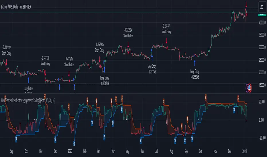
Session Breakout Scalper Trading BotHi Traders !
Introduction:
I have recently been exploring the world of automated algorithmic trading (as I prefer more objective trading strategies over subjective technical analysis (TA)) and would like to share one of my automation compatible (PineConnecter compatible) scripts “Session Breakout Scalper”.
The strategy is really simple and is based on time conditional breakouts although has more ”relatively” advanced optional features such as the regime indicators (Regime Filters) that attempt to filter out noise by adding more confluence states and the ATR multiple SL that takes into account volatility to mitigate the down side risk of the trade.
What is Algorthmic Trading:
Firstly what is algorithmic trading? Algorithmic trading also known as algo-trading, is a method of using computer programs (in this case pine script) to execute trades based on predetermined rules and instructions (this trading strategy). It's like having a robot trader who follows a strict set of commands to buy and sell assets automatically, without any human intervention.
Important Note:
For Algorithmic trading the strategy will require you having an essential TV subscription at the minimum (so that you can set alerts) plus a PineConnecter subscription (scroll down to the .”How does the strategy send signals” headings to read more)
The Strategy Explained:
Is the Time input true ? (this can be changed by toggling times under the “TRADE MEDIAN TIMES” group for user inputs).
Given the above is true the strategy waits x bars after the session and then calculates the highest high (HH) to lowest low (LL) range. For this box to form, the user defined amount of bars must print after the session. The box is symmetrical meaning the HH and LL are calculated over a lookback that is equal to the sum of user defined bars before and after the session (+ 1).
The Strategy then simultaneously defines the HH as the buy level (green line) and the LL as the sell level (red line). note the strategy will set stop orders at these levels respectively.
Enter a buy if price action crosses above the HH, and then cancel the sell order type (The opposite is true for a stop order).
If the momentum based regime filters are true the strategy will check for the regime / regimes to be true, if the regime if false the strategy will exit the current trade, as the regime filter has predicted a slowing / reversal of momentum.
The image below shows the strategy executing these trading rules ( Regime filters, "Trades on chart", "Signal & Label" and "Quantity" have been omitted. "Strategy label plots" has been switched to true)
Other Strategy Rules:
If a new session (time session which is user defined) is true (blue vertical line) and the strategy is currently still in a trade it will exit that trade immediately.
It is possible to also set a range of percentage gain per day that the strategy will try to acquire, if at any point the strategy’s profit is within the percentage range then the position / trade will be exited immediately (This can be changed in the “PERCENT DAY GAIN” group for user inputs)
Stops and Targets:
The strategy has either static (fixed) or variable SL options. TP however is only static. The “STRAT TP & TP” group of user inputs is responsible for the SL and TP values (quoted in pips). Note once the ATR stop is set to true the SL values in the above group no longer have any affect on the SL as expected.
What are the Regime Filters:
The Larry Williams Large Trade Index (LWLTI): The Larry Williams Large Trade Index (LWTI) is a momentum-based technical indicator developed by iconic trader Larry Williams. It identifies potential entries and exits for trades by gauging market sentiment, particularly the buying and selling pressure from large market players. Here's a breakdown of the LWTI:
LWLTI components and their interpretation:
Oscillator: It oscillates between 0 and 100, with 50 acting as the neutral line.
Sentiment Meter: Values above 75 suggest a bearish market dominated by large selling, while readings below 25 indicate a bullish market with strong buying from large players.
Trend Confirmation: Crossing above 75 during an uptrend and below 25 during a downtrend confirms the trend's continuation.
The Andean Oscillator (AO) : The Andean Oscillator is a trend and momentum based indicator designed to measure the degree of variations within individual uptrends and downtrends in the prices.
Regime Filter States:
In trading, a regime filter is a tool used to identify the current state or "regime" of the market.
These Regime filters are integrated within the trading strategy to attempt to lower risk (equity volatility and/or draw down). The regime filters have different states for each market order type (buy and sell). When the regime filters are set to true, if these regime states fail to be true the trade is exited immediately.
For Buy Trades:
LWLTI positive momentum state: Quotient of the lagged trailing difference and the ATR > 50
AO positive momentum state: Bull line > Bear line (signal line is omitted)
For Sell Trades:
LWLTI negative momentum stat: Quotient of the lagged trailing difference and the ATR < 50
AO negative momentum state: Bull line < Bear line (signal line is omitted)
How does the Strategy Send Signals:
The strategy triggers a TV alert (you will neet to set a alert first), TV then sends a HTTP request to the automation software (PineConnecter) which receives the request and then communicates to an MT4/5 EA to automate the trading strategy.
For the strategy to send signals you must have the following
At least a TV essential subscription
This Script added to your chart
A PineConnecter account, which is paid and not free. This will provide you with the expert advisor that executes trades based on these strategies signals.
For more detailed information on the automation process I would recommend you read the PineConnecter documentation and FAQ page.
Dashboard:
This Dashboard (top right by defualt) lists some simple trading statistics and also shows when a trade is live.
Important Notice:
- USE THIS STRATEGY AT YOUR OWN RISK AND ALWAYS DO YOUR OWN RESEARCH & MANUAL BACKTESTING !
- THE STRATEGY WILL NOT EXHIBIT THE BACKTEST PERFORMANCE SEEN BELOW IN ALL MARKETS !
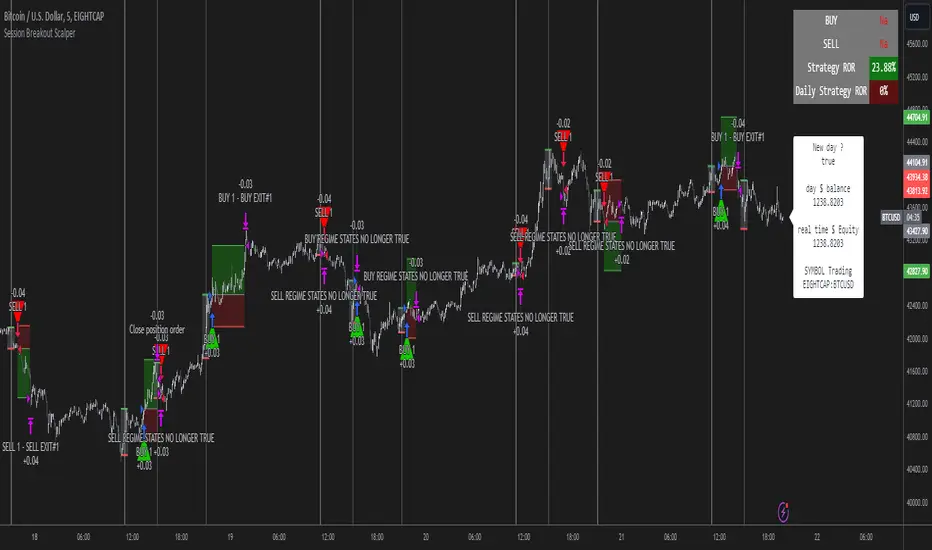
IchiBot - [SigmaStreet]
The IchiBot Indicator has been used to develop automated trading systems. It leverages the open-source Ichimoku framework provided by Trading View, to enable users to creatively generate over 1 trillion different combinations of trading conditions with the use of multiple timeframes to create unique “signal labels” that can be used to create custom strategies or provide in depth market analysis. At the end of this description, I have provided an example of input settings for a simple scalping strategy that I have back tested on US30 on the 5 minute timeframe.
Overview of the Settings:
The visuals section includes an option to show or hide certain parts of the indicator and change the size of the signal labels plotted on the chart.
Next to the “Signal color on baseline/candles” section, you can choose if you want to see additional signals generations from the most previous plotted label on a color changing baseline, or color changing candles. A color change from gray to blue/red indicate that the conditions from the most previously plotted signal label have been met again.
The next 5 sections are all related to the strategy portion of the indicator, used to aid in the back testing process. These sections are titled “Stop loss”, “Take Profit”, “Trail Stop”, “Trade Settings” and “Trade Schedule”.
The Stop Loss section includes an option to choose between value of “pts”, “atr” (average true range) or “None”. The stop loss value in “pts” is simply a specified number of points or pips from the current entry price of a trade that are input in the “SL” section. If the stop loss type is “atr” the “SL” section is not used and the value is calculated and displaced from the current entry price of a trade based on the atr period multiplied by the atr multiplier.
The take profit section is based on the same logic as the stop loss.
The Trail Stop section includes an option to choose between values “pts” or “None”. If the Trail Stop value is “pts”, a trailing stop loss is activated if a trade moves a point value into profit that exceeds the value of the “Trail Activation”. If the Trail Offset type is “pts”, the trailing stop loss is placed a point value away from the current price that is equal to the “Trail Offset” value.
The trade settings section has two options to either prevent or allow trade reversals and prevent or allow only 1 trade per signal label.
If the “Don’t allow trade reversals” is on, then a currently active trade can not be cancelled by an opposite trade signal. It can only be cancelled by the exit logic selected in the above sections. If the “One trade per signal” is selected, the strategy will only enter a trade if the most recent signal label is different from the last signal label where a trade was entered, or if the most recent signal label is in the opposite direction of the most recent signal label where a trade was entered.
The trade schedule section includes an option to only generate signal labels during the specified time. You can choose between 24/7 which will generate signals without any time restriction, or you can choose a custom time which is based on the America / New York time zone.
The timeframe settings section includes an option to choose “single” or “multiple” timeframes, as well as an option to show every signal label combination (“all”), or only the signal labels with the highest numerical value (“absolute”).
If you select “single” next to “timeframe”, the indicator will show you labels based on trade conditions met from only 1 selected timeframe. If you select “multiple” next to “timeframe”, the indicator is designed to return signal labels based on trade conditions that have been met on at least 2 different timeframes.
If you select “multiple” and “use current timeframe”, the indicator will include labels that always include a minimum of 2 timeframes where 1 timeframe is always the current timeframe. If you unselect the “use current timeframe”, the indicator will include labels with a minimum of 2 timeframes.
If you select “multiple” next to “timeframe” and “all” next to “Show all/absolute labels”, the indicator will show you every possible combination of labels that vary from trade conditions met on a minimum of 2 timeframes, to the maximum number of timeframes selected.
If you select “multiple” next to “timeframe” and “absolute” next to “Show all/absolute labels”, the indicator will only show you labels where the numerical value is equivalent to the maximum number of timeframes selected.
Each signal label provides a number which refers to the number of timeframes used to generate the label, offering insights briefly. Hover over a label to reveal detailed tooltip information that details the exact timeframes used to generate each label.
You can choose all from “Show all/absolute labels” to see every possible combination of trade signals or “absolute” to only see labels that have the highest possible numerical value. Absolute means that every condition selected from every timeframe was calculated to be true at the same time on the same candle.
The next 8 sections are “Current timeframe trade conditions”, “1-minute timeframe trade conditions”, “5-minute timeframe trade conditions”, “15-minute timeframe trade conditions”, “30-minute timeframe trade conditions”, “1-hour timeframe trade conditions”, “4-hour timeframe trade conditions”, “Daily timeframe trade conditions”.
These sections include the same 10 trade conditions, that can be used independently, or in combination with each other. This brings the total number of trade conditions to 70.
The final section includes a standard option to adjust the current Ichimoku values.
Understanding the Calculations:
The term “future” refers to a value that is calculated 26 candles to the right of the most recent closing price.
The term “current” refers to a value that is calculated on the most recent closing price.
The term “past” refers to a value that is calculated 26 candles to the left of the most recent closing price.
Bullish is referred to as “blue” and bearish is referred to as “red”.
Buy Signals:
1. The current closing price is greater than the current cloud value.
2. The future cloud is blue.
3. The current closing price is greater than the current conversion line.
4. The current conversion line is greater than the current baseline.
5. The lagging span is greater than the closing price of the last 25 candles.
6. The lagging span is greater than the past cloud.
7. The lagging span is greater than the past conversion line and the past baseline.
8. The current conversion line is greater than the current cloud.
9. The current baseline is greater than the current cloud.
10. The value of the current cloud to the future cloud is completely blue.
Sell Signals:
1. The current closing price is less than the current cloud value.
2. The future cloud is red.
3. The current closing price is less than the current conversion line.
4. The current conversion line is less than the current baseline.
5. The lagging span is less than the closing price of the last 25 candles.
6. The lagging span is less than the past cloud.
7. The lagging span is less than the past conversion line and the past baseline.
8. The current conversion line is less than the current cloud.
9. The current baseline is less than the current cloud.
10. The value of the current cloud to the future cloud is completely red.
The script enables users to access the value of these 10 trade conditions across the 7 major time frames (1-minute, 5-minute, 15-minute, 30-minute, 1-hour, 4-hour, Daily, and the current charts time frame) by using the official non repainting request security function provided by Trading View:
f_secSecurity(_src, _res, _exp) =>
request.security(_src, _res, _exp )
This indicator provides up to 70 variables (10 variables X 7 timeframes) that can be used separately, or in combination to generate signal labels.
Enhance your visual analysis with a color-changing baseline and candle colors that adapt to signal shifts, offering an immediate understanding of market trends. The base line will change from gray to blue/red which will reference the most previously plotted signal label. This change in color indicate that the conditions from the most recently plotted signal label have been met once again. Please refer to the example below.
Adjustments to the Ichimoku Indicator:
The script uses a slightly refined version of the Ichimoku indicator to calculate 10 different “trade conditions”. Each trade condition can create 1 bullish signal label and 1 bearish signal label. The calculations are primarily based on “greater than and less than logic” which is standard for signal generation.
In the original Ichimoku calculations, the “Lagging Span” has a default value of 26 periods. In the actual calculations, this input with the title “Lagging Span” is referred to as the “displacement”. When the lagging span is plotted on the chart, it is plotted with an offset value of offset = -displacement + 1 which technically plots the lagging span 25 candles to the left the most recent candle (if you count the most recent closing price as 0 and not 1). The clouds are plotted with an offset of offset = displacement -1 which technically plots the clouds 25 candles to the right of the most recent candle.
I have adjusted the logic of the Ichimoku indicator so the lagging span is still plotted 25 candles to the left of the most recently confirmed candle close, but the cloud is plotted 26 candles to the right of the most recent confirmed candle close.
This seemingly small adjustment of one candle cannot simply be adjusted in the settings of the original Ichimoku indicator since the calculations of the cloud and lagging span displacements are directly affected by the same value (displacement = 26, also known as the “lagging span”). My script is adjusted to make calculations where the lagging span is 25 candles to the left of the most recent candle, and the cloud is displaced 26 candles to the right of the most recent candle.
For example, my scripts logic to detect if the current closing price is over the current cloud is (close > leadLead1 and close > leadLine2 and leadLine1 > leadLine2 . By using a lookback of , the logic assumes that the displaced value is 26 bars to the right of the most recent candle. My script also reflects this logic in the plotted values of the cloud where the offset values are offset = displacement. This adjustment is made without affecting any other part of the Ichimoku indicators calculations, only the displacement of the cloud which directly affects the logic of trade conditioins. This change is a deliberate and necessary function of this script’s logic to generate trade conditions and signal labels.
I’ve removed the conversion line and the lagging span and introduced a 26-period pivot high/low to provide a less cluttered chart. The pivot high/low looks 26 periods to the left and only 1 period to the right. The lagging span and conversion line logic is still built into the framework of the trading signals. If you choose to enable the lagging span, or conversion line.
trading approach, and always test your strategies thoroughly.
The function to generate the "Signal Labels" calculates every single possible combination of the 7 different timeframes which is a total of 127 combinations for bullish signal labels, and 127 combinations for bearish signal labels. This function also provides the necessary criteria for the strategy entry conditions, based on the dynamically calculated values derived from the signal labels themselves. For example: "buy signal on 1 minute and 5 minute timeframe" is considered 1 combination, and "Buy signal on current, 5 minute, 15 minute, 30 minute, 1 hour, 4 hour and daily timeframe" is also considered 1 combination. There are a total of 254 combinations between buy and sell signal labels along with 254 individual variables with their own unique tool tip description. The signal label function alone spans over 1340 lines of code (minus spaces and comments) to specifically account for every possible variable combination. This unique and original function also calculates the signal label "value" which is the number you see on the signal label. This function adjusts the amount of labels plotted, the value and description of all labels based on the timeframe settings "single"/"multiple", the use of "use current timeframe" setting, and the "trade schedule". This signal label function has been a landmark piece of code for me in my endeavor to create and optimize my strategies based on its ability to provide an in depth analysis of the timeframes used when generating signal labels. This function is main reason that this script has been published closed source.
Back tested results.
The current results are from US30 (Dow Jones Industrial Average CFD) on the 5-minute timeframe using regular candles. The inputs are as follows:
Stop loss = 5000 pts
No take profit.
Trail activation = 100 pts
Trail offset = 100 pts
Don’t allow trade reversals
Trade 24/7
Timeframe = multiple
Show absolute signals
Use current timeframe, lag span over/under candles
Use 30m timeframe, all cloud is bull/bear
Initial capital = $10,000 USD, 1 contract, $0.07 per contract, slippage = 3 ticks, use bar magnifier = on
Timeframe = June 1st, 2023 – November 10th, 2023, risk = 5% (greatest loosing trade = $500.44)
[Round Numbers] Signal Clean Up Analysis with Backtest (TSO)Round Numbers NEW GEN indicator!
===========================================================================
===========================================================================
This is a full-cycle trading system indicator - it will show and alert each step of the trade from open to close. The algorithm here uses Round Numbers for generating signals, TP (Take Profit) and SL (Stop Loss) levels. Round numbers play big role in trading and can easily become strong support and resistance levels where price can bounce and go the opposite way or go through with a very nice run afterwards.
In addition there is a chained (NOTE: You can select several or ALL of the features, this is not limited to either one) signal cleanup and analysis approach with scheduling and alerting capabilities. Works with most popular timeframes: 1M, 3M, 5M, 15M, 30M, 1H, 4H, D.
NOTE: Every action of the trade is calculated on a confirmed closed candle bar state (barstate.isconfirmed), so the indicator will never repaint!
NOTE: At position open - there will be calculated Take-Profit and Stop-Loss targets, however each target is considered hit, when candle bar closes breaking that target, so Take-Profit and Stop-Loss when hit will slightly differ then what you see at trade/position open.
===========================================================================
===========================================================================
Round Numbers up|down unit setting and overall explanation
---------------------------------------------------------------------------
Round Number up|down unit: is the distance between round numbers on the chart. Since these round number levels are also used by the algorithm to open/close trades, it is important to set this setting to a logical number, which will correspond to an average price movement of the instrument.
Here are some examples for a few popular instruments on what will the default 1 round number unit correspond to and what would be suggested:
BTCUSD > $1 (this won't work for Bitcoin, try at least $100 - 100units)
SPY: > $1 (one of the best settings for SPY or QQQ, 50cents shows good results as well - 0.5units)
FOREX (all major pairs): > 10PIPs (that may be a bit small, unless scalping, try 50PIPs - 5units)
===========================================================================
===========================================================================
Explanation of all the Features | Strategy Configuration Guide | Indicator Settings | Signal Cleanup Analysis
---------------------------------------------------------------------------
>>> Customizable Backtesting for a specific date range, results via TradingView strategy, which includes “Deep Backtesting” for largest amounts of data on trading results.
>>> Trading Schedule with customizable trading daily time range, automatic closing/alert trades before Power Hour or right before market closes or leave it open until next day.
>>> 3 Trading Systems.
>>> Static/Dynamic/Trailing Take-Profit and Stop-Loss setups (HIGHLIGHT: Stop-Loss will be moved to Entry after TP1 is taken or a smart trailing Stop-Loss can be used with Stop-Loss dynamically following the trade to minimize risk).
>>> Single or Multiple profit targets (up to 5).
>>> Take-Profit customizable offset feature (set your Take-Profit targets slightly before everyone is expecting it!).
>>> Candle bar signal analysis (matching candle color, skip opposite structured and/or doji candle uncertain signals).
>>> Additional analysis of VWAP/EMA/ATR/EWO (Elliot Wave Oscillator)/Divergence MACD+RSI/Volume signal confirmation (clean up your chart with indicator showing only the best potential signals!).
>>> Advanced Alerts setup, which can be potentially setup with a trading bot over TradingView Webhook (NOTE: This will require advanced programming knowledge).
===========================================================================
Labels, plots, colors explanations:
---------------------------------------------------------------------------
>>>>> LONG open: green "house" looking arrow below candle bar.
>>>>> SHORT open: red "house" looking arrow above candle bar.
>>>>> LONG/SHORT take-profit target: green/red circles (multi-profit > TP2/3/4/5 smaller circles).
>>>>> LONG/SHORT stop-loss target: green/red + crosses.
>>>>> LONG/SHORT take-profit hits: green/red diamonds.
>>>>> LONG/SHORT stop-loss hits: green/red X-crosses.
>>>>> LONG/SHORT EOD (End of Day | Intraday style) close (profitable trade): green/red squares.
>>>>> LONG/SHORT EOD (End of Day | Intraday style) close (loss trade): green/red PLUS(+)-crosses.
===========================================================================
Date Range and Trading Schedule Settings
---------------------------------------------------------------------------
>>>>> Date Range: Select your start and/or end dates (uncheck “End” for indicator to show results up to the very moment and to use for LIVE trading) for backtesting results, if not using backtesting – uncheck “Start”/“End” to turn it off.
>>>>> Use TradingView “Strategy Tester” to see backtesting results
NOTE: If Strategy Tester does not show any results with Date Ranged fully unchecked, there may be an issue where a script opens a trade, but there is not enough TradingView power to set the Take-Profit and Stop-Loss and somehow an open trade gets stuck and never closes, so there are “no trades present”. In such case you will need to manually check “Start”/“End” dates or use “Depp Backtesting” feature!
>>>>> Trading Schedule: This is where you can setup Intraday Session or any custom session schedule you wish. Turn it ON. Select trading hours. Select EOD (End of Day) setting (NOTE: If it will be OFF, the indicator will assume you are holding your position open until next day!). Please note the EOD trade closure times with the 2 different Intraday close settings when turned on:
At Market Close:
1/3/5min > will close at 15:55pm ET
15min > will close at 15:45pm ET
30min > will close at 15:30pm ET
45min > will close at 15:45pm ET
60min > will close at 15:00pm ET
Before Power Hour:
1/3/5min > will close at 15:00pm ET
15min > will close at 15:00pm ET
30min > will close at 15:00pm ET
45min > will close at 15:00pm ET
60min > will close at 15:00pm ET
>>> Trading Systems: 1) "Open Until Closed by TP or SL": the signal will only open a trade if no trades are currently open/trunning, a trade can only be closed by Take Profit, Stop Loss or End of Day close (if turned on) | 2) "Open Until Closed by TP or SL + OCA": Same as 1), but if there is an opposite signal to the trade which is currently open > it will immediately be closed with new trade open or End of Day close (if turned on) | 3) "OCA (no TP or SL)": There are is Take Profit or Stop Loss, only an opposite signal will close current trade and open an opposite one or End of Day close (if turned on).
>>> Turn On/Off: Current Position SL + Opposite Position Open Signal on the same closing candle bar (If current trade hits Stop-Loss and at that same closing candle bar there is a signal for an opposite direction trade > indicator will close current position as Stop-Loss and immediately open an opposite position). NOTE: With this option turned on, there will be more trades, but not necessarily better results, since after Stop-Loss is hit, it may make sense to wait a little before opening an opposite trade, even if it matches the condition at the same time when Stop-Loss is hit, but sometimes it shows great results, so this setting/feature is included. NOTE: This setting only will work/make sense with TP and SL style/behavior both be set to "Fully Closed Candle"!
>>> Turn On/Off: Turn On/Off: Current Position REGULAR SL | Only the SL + Opposite Position Open will trigger if turned on, IF NOT - THERE WILL BE NO STOP-LOSS AT ALL!!! NOTE: It is very dangerous to trade without Stop-Loss!
>>>>> Signal Candle Bar consuming Take-Profits - position/trade signal candle bar is big enough to "consume"/close ahead the first TP setting > the signal can either be skipped, or all Take-Profit areas pushed ahead using smart formula)
>>>>> MULTIPROFIT | TP (Take-Profit) System: 1) Static – Once the trade is open, all Take-Profit target(s) are immediately calculated and set for the trade > once the target(s) is hit > trade will be partially closed (if candle bar closes beyond several Take-Profit targets > trade will be reduced accordingly to the amount of how many Take-Profit targets were hit) ||| 2) Dynamic – Once the trade is open, only the 1st Take-Profit target is calculated, once the 1st Take-Profit is hit > next Take-Profit distance is calculated based on the distance from trade Entry to where 1st Take-Profit was taken, once 2nd Take-Profit is taken > 3rd Take-Profit is calculated per same logic, these are good for price momentum as with price speeding up – profits increase as well!
>>>>> MULTIPROFIT: SL (stop loss) System | Static: SL is set at position open and remains such; Dynamic: Once ANY TP is taken > SL will be moved to Entry; Trailing: SL will be moved along the position (smart trailing stop-loss), at TP1 taken > SL moves to Entry, at TP2 taken > SL moves to TP1, at TP3 taken > SL moves to TP2 and so on.
>>>>> # of TPs (number of take profit targets): Just like it is named, this is where you select the number of Take-Profit targets for your trading system (NOTE: If "OCA (no TP or SL)" Trading System is selected, this setting won’t do anything, since there are no TP or SLs for that system).
>>>>> TP(s) offset: This is a special feature for all Take-Profit targets, where you can turn on a customizable offset, so that if the price is almost hitting the Take-Profit target, but never actually touches it > you will capture it. This is good to use with HHLL (Highest High Lowest Low), which is pretty much a Support/Resistance as often the price will nearly touch these strong areas and turn around…
===========================================================================
Dynamic/Static/Trailing Take-Profit and Stop-Loss visual examples:
---------------------------------------------------------------------------
1) Fully Static Take-Profit and Stop-Loss
This one is a fully static setup for both Take-Profit and Stop-Loss, you can also observe how trade is closed right before the Power Hour (trade can be closed right before Power Hour or right before Market Closes or left overnight as desired).
2) Static/Dynamic, Static Take-Profit and Dynamic Stop-Loss
You can see a static Take-Profit set at position open, while Stop-Loss moves to Entry once TP1 target is taken.
3) Static/Trailing, Static Take-Profit and Trailing Stop-Loss
In here with each Take-Profit taken, Stop-Loss moves along the trade to previous Take-Profit level, you can notice how stop-loss literally follows the trade and reduces the potential loss.
4) Dynamic/Trailing, Dynamic Take-Profit and Trailing Stop-Loss
See how Take-Profit distances increase with price momentum. Just like in previous example - Trailing Stop-Loss is following the trade and reducing the riks.
===========================================================================
Signal Analysis and Cleanup Settings
---------------------------------------------------------------------------
>>>>> Candle Analysis | Candle Color signal confirmation: If closed candle bar color does not match the signal direction > no trade will be open.
>>>>> Candle Analysis | Skip opposite candle signals: If closed candle bar color will match the signal direction, but candle structure will be opposite (for example: bearish green hammer, long high stick on top of a small green square) > no trade will be open.
>>>>> Candle Analysis | Skip doji candle signals: If closed candle bar will be the uncertain doji > no trade will be open.
>>>>> Divergence/Oscillator Analysis | EWO (Elliot Wave Oscillator) signal confirmation: LONG will only be open if at signal, EWO is green or will be at bullish slope (you can select which setting you desire), SHORT if EWO is red or will be at bearish slope.
>>>>> Divergence/Oscillator Analysis | VWAP signal confirmation: LONG will only be open if at signal, the price will be above VWAP, SHORT if below.
>>>>> Divergence/Oscillator Analysis | Moving Average signal confirmation: LONG will only be open if at signal, the price will be above selected Moving Average, SHORT if below.
>>>>> Divergence/Oscillator Analysis | ATR signal confirmation: LONG will only be open if at signal, the price will be above ATR, SHORT if below.
>>>>> Divergence/Oscillator Analysis | RSI + MACD signal confirmation: LONG will only be open if at signal, RSI + MACD will be bullish, SHORT if RSI + MACD will be bearish.
>>>>> Volume signal confirmation: LONG/SHORT will only be opened with strong Volume matching the signal direction, by default, strong Volume percentage is set to 150% and weak to 50%, but you can change it as you desire.
===========================================================================
||||||||||||||||||||||||||||||||||| *** ||||||||||||||||||||||||||||||||||| *** |||||||||||||||||||||||||||||||||||
||||||||||||||||||||||||||||||||||| *** ||||||||||||||||||||||||||||||||||| *** |||||||||||||||||||||||||||||||||||
TP System - VERY IMPORTANT INFO!
-------------------------------------------------------------------------------------------------------------------
"TP PERCENTAGE" - amount by which current trade/position needs to be reduced/partially closed/sold.
-------------------------------------------------------------------------------------------------------------------
TP System: Dynamic
"TP PERCENTAGE" - will always be the same amount (trade/position size divided by the # of take-profit(TP) targets) and percentage to be closed will always be of the ORIGINAL trade/position.
-------------------------------------------------------------------------------------------------------------------
TP System: Static
"TP PERCENTAGE" - will always be the same amount IF take-profit(TP) targets are hit 1-by-1 (TP1 > TP2 > TP3 > TP4 > TP5), otherwise it will vary and unless it is a 1st take-profit(TP1), the REMAINING trade/position size will always be smaller than original and therefore the percentage to be closed will always be of the REMAINING trade/position and NOT the original one!
-------------------------------------------------------------------------------------------------------------------
"TP PERCENTAGE" CheatSheet (these are the only percentages you may see)
-----------------------------------------------------------------------
TP PERCENTAGE---Close/Sell Amount-------------Example (trade size: 50 stocks)
20%-------------trade size * 0.2--------------50 * 0.2 = 10 stocks
25%-------------trade size * 0.25-------------50 * 0.25 = 12.5(~13) stocks
34%-------------trade size * 0.34-------------50 * 0.34 = 17 stocks
40%-------------trade size * 0.4--------------50 * 0.4 = 20 stocks
50%-------------trade size * 0.5--------------50 * 0.5 = 25 stocks
60%-------------trade size * 0.6--------------50 * 0.6 = 30 stocks
66%-------------trade size * 0.66-------------50 * 0.66 = 33 stocks
75%-------------trade size * 0.75-------------50 * 0.75 = 37.5(~38) stocks
80%-------------trade size * 0.8--------------50 * 0.8 = 40 stocks
100%------------trade size--------------------50 = 50 stocks
-----------------------------------------------------------------------
If for any reason a portion of the current/remaining trade closed at such occurrence was slightly wrong, it is not an issue. Such occurrences are rare and with slight difference in partial TP closed is not significant to overall performance of our algorithms.
||||||||||||||||||||||||||||||||||| *** ||||||||||||||||||||||||||||||||||| *** |||||||||||||||||||||||||||||||||||
||||||||||||||||||||||||||||||||||| *** ||||||||||||||||||||||||||||||||||| *** |||||||||||||||||||||||||||||||||||
Alert Settings (you don’t have to touch this section unless you will be using TradingView alerts through a Webhook to use with trading bot)
---------------------------------------------------------------------------
Here is how a LONG OPEN alert looks like.
NOTE: Each label , , etc. is customizable, you can change the text of it within indicator Input settings.
ALERT >>>>>>>>>>>>>>>>>>>>>>>>>>>>>>>>>>>>>>>>>>>>>>>
COIN: BTCUSD
TIMEFRAME: 15M
LONG: OPEN
ENTRY: 20000
TP1: 20500
TP2: 21000
TP3: 21500
TP4: 22500
TP5: 23500
SL: 19000
Leverage: 0
---------------------------------------------------------------------------
Here is how a TP1 alert will look with 5 TPs breakdown of the trade.
NOTE1: Next to TP1 taken it will show at which price it was triggered.
NOTE2: Next to "TP Percentage" it shows how much of the CURRENT/ACTIVE/REMAINING trade needs to be closed.
NOTE2: If TP2/3/4/5 comes before TP1 - the alert will tell you exactly how many percent of the trade needs to be closed!
ALERT >>>>>>>>>>>>>>>>>>>>>>>>>>>>>>>>>>>>>>>>>>>>>>>
COIN: BTCUSD
TIMEFRAME: 15M
LONG: TP1
TP1: 20500
TP Percentage: 20%
---------------------------------------------------------------------------
Here is how an alert will look for LONG - STOP-LOSS.
ALERT >>>>>>>>>>>>>>>>>>>>>>>>>>>>>>>>>>>>>>>>>>>>>>>
COIN: BTCUSD
TIMEFRAME: 15M
ENTRY: 20000
LONG: SL
SL: 19000
---------------------------------------------------------------------------
Here is how an alert will look for LONG - EOD (End of Day) In Profit close.
ALERT >>>>>>>>>>>>>>>>>>>>>>>>>>>>>>>>>>>>>>>>>>>>>>>
COIN: BTCUSD
TIMEFRAME: 15M
LONG: EOD-Close (profit)
ENTRY: 20000
EOD-Close: 21900
===========================================================================
Adding Alerts in TradngView
---------------------------------------------------------------------------
-Add indicator to chart and make sure the correct strategy is configured (check Backtesting results)
-Right-click anywhere on the TradingView chart
-Click on Add alert
-Condition: Select this indicator by it’s name
-Immediately below, change it to "alert() function calls only", as other wise there will be 2 alerts for every alert!
-Expiration: Open-ended (that may require higher tier TradingView account, otherwise the alert will need to be occasionally re-triggered)
-Alert name: Whatever you desire
-Hit “Create”
-Note: If you change ANY Settings within the indicator – you must DELETE the current alert and create a new one per steps above, otherwise it will continue triggering alerts per old Settings!
===========================================================================
If you have any questions or issues with the indicator, please message me directly via TradingView.
---------------------------------------------------------------------------
Good Luck! (NOTE: Trading is very risky, past performance is not necessarily indicative of future results, so please trade responsibly!)
---------------------------------------------------------------------------
NOTE: There seems to be a strange glitch when strategy is running live, it will show "double-take" take-profits labels on the chart. This is not affecting the script logic and backtesting results, if you simply change the timeframe real quick to something else then back - it will no longer show the duplicate orders... this must be some sort of a glitch as every alert was thoroughly tested to make sure everything is working!
