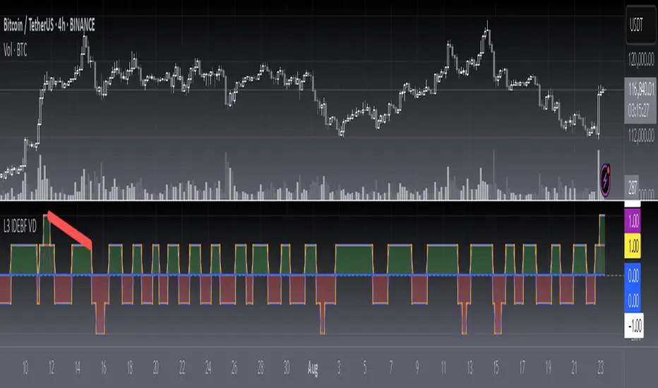
Pattern Forecast (Expo)█ Overview
The Pattern Forecast indicator is a technical analysis tool that scans historical price data to identify common chart patterns and then analyzes the price movements that followed these patterns. It takes this information and projects it into the future to provide traders with potential price actions that may occur if the same pattern is identified in real-time market data. This projection helps traders to understand the possible outcomes based on the previous occurrences of the pattern, thereby offering a clearer perspective of the market scenario. By analyzing the historical data and understanding the subsequent price movements following the appearance of a specific pattern, the indicator can provide valuable insights into potential future market behavior.
█ Calculations
The indicator works by scanning historical price data for various candlestick patterns. It includes all in-built TradingView patterns, credit to TradingView that has coded them.
Essentially, the indicator takes the historical price moves that followed the pattern to forecast what might happen next.
█ Example
In this example, the algorithm is set to search for the Inverted Hammer Bullish candlestick pattern. If the pattern is found, the historical outcome is then projected into the future. This helps traders to understand how the past pattern evolved over time.
█ How to use
Providing traders with a comprehensive understanding of historical patterns and their implications for future price action allows them to assess the likelihood of specific market scenarios objectively. For example, suppose the pattern forecast indicator suggests that a particular pattern is likely to lead to a bullish move in the market. A trader might consider going long if the same pattern is identified in the real-time market. Similarly, a trader might consider shorting the asset if the indicator suggests a bearish move is likely, if the same pattern is identified in the real-time market.
█ Settings
Pattern
Select the pattern that the indicator should scan for. All inbuilt TradingView patterns can be selected.
Forecast Candles
Number of candles to project into the future.
-----------------
Disclaimer
The information contained in my Scripts/Indicators/Ideas/Algos/Systems does not constitute financial advice or a solicitation to buy or sell any securities of any type. I will not accept liability for any loss or damage, including without limitation any loss of profit, which may arise directly or indirectly from the use of or reliance on such information.
All investments involve risk, and the past performance of a security, industry, sector, market, financial product, trading strategy, backtest, or individual's trading does not guarantee future results or returns. Investors are fully responsible for any investment decisions they make. Such decisions should be based solely on an evaluation of their financial circumstances, investment objectives, risk tolerance, and liquidity needs.
My Scripts/Indicators/Ideas/Algos/Systems are only for educational purposes!
In den Scripts nach "algo" suchen
Quinn-Fernandes Fourier Transform of Filtered Price [Loxx]Down the Rabbit Hole We Go: A Deep Dive into the Mysteries of Quinn-Fernandes Fast Fourier Transform and Hodrick-Prescott Filtering
In the ever-evolving landscape of financial markets, the ability to accurately identify and exploit underlying market patterns is of paramount importance. As market participants continuously search for innovative tools to gain an edge in their trading and investment strategies, advanced mathematical techniques, such as the Quinn-Fernandes Fourier Transform and the Hodrick-Prescott Filter, have emerged as powerful analytical tools. This comprehensive analysis aims to delve into the rich history and theoretical foundations of these techniques, exploring their applications in financial time series analysis, particularly in the context of a sophisticated trading indicator. Furthermore, we will critically assess the limitations and challenges associated with these transformative tools, while offering practical insights and recommendations for overcoming these hurdles to maximize their potential in the financial domain.
Our investigation will begin with a comprehensive examination of the origins and development of both the Quinn-Fernandes Fourier Transform and the Hodrick-Prescott Filter. We will trace their roots from classical Fourier analysis and time series smoothing to their modern-day adaptive iterations. We will elucidate the key concepts and mathematical underpinnings of these techniques and demonstrate how they are synergistically used in the context of the trading indicator under study.
As we progress, we will carefully consider the potential drawbacks and challenges associated with using the Quinn-Fernandes Fourier Transform and the Hodrick-Prescott Filter as integral components of a trading indicator. By providing a critical evaluation of their computational complexity, sensitivity to input parameters, assumptions about data stationarity, performance in noisy environments, and their nature as lagging indicators, we aim to offer a balanced and comprehensive understanding of these powerful analytical tools.
In conclusion, this in-depth analysis of the Quinn-Fernandes Fourier Transform and the Hodrick-Prescott Filter aims to provide a solid foundation for financial market participants seeking to harness the potential of these advanced techniques in their trading and investment strategies. By shedding light on their history, applications, and limitations, we hope to equip traders and investors with the knowledge and insights necessary to make informed decisions and, ultimately, achieve greater success in the highly competitive world of finance.
█ Fourier Transform and Hodrick-Prescott Filter in Financial Time Series Analysis
Financial time series analysis plays a crucial role in making informed decisions about investments and trading strategies. Among the various methods used in this domain, the Fourier Transform and the Hodrick-Prescott (HP) Filter have emerged as powerful techniques for processing and analyzing financial data. This section aims to provide a comprehensive understanding of these two methodologies, their significance in financial time series analysis, and their combined application to enhance trading strategies.
█ The Quinn-Fernandes Fourier Transform: History, Applications, and Use in Financial Time Series Analysis
The Quinn-Fernandes Fourier Transform is an advanced spectral estimation technique developed by John J. Quinn and Mauricio A. Fernandes in the early 1990s. It builds upon the classical Fourier Transform by introducing an adaptive approach that improves the identification of dominant frequencies in noisy signals. This section will explore the history of the Quinn-Fernandes Fourier Transform, its applications in various domains, and its specific use in financial time series analysis.
History of the Quinn-Fernandes Fourier Transform
The Quinn-Fernandes Fourier Transform was introduced in a 1993 paper titled "The Application of Adaptive Estimation to the Interpolation of Missing Values in Noisy Signals." In this paper, Quinn and Fernandes developed an adaptive spectral estimation algorithm to address the limitations of the classical Fourier Transform when analyzing noisy signals.
The classical Fourier Transform is a powerful mathematical tool that decomposes a function or a time series into a sum of sinusoids, making it easier to identify underlying patterns and trends. However, its performance can be negatively impacted by noise and missing data points, leading to inaccurate frequency identification.
Quinn and Fernandes sought to address these issues by developing an adaptive algorithm that could more accurately identify the dominant frequencies in a noisy signal, even when data points were missing. This adaptive algorithm, now known as the Quinn-Fernandes Fourier Transform, employs an iterative approach to refine the frequency estimates, ultimately resulting in improved spectral estimation.
Applications of the Quinn-Fernandes Fourier Transform
The Quinn-Fernandes Fourier Transform has found applications in various fields, including signal processing, telecommunications, geophysics, and biomedical engineering. Its ability to accurately identify dominant frequencies in noisy signals makes it a valuable tool for analyzing and interpreting data in these domains.
For example, in telecommunications, the Quinn-Fernandes Fourier Transform can be used to analyze the performance of communication systems and identify interference patterns. In geophysics, it can help detect and analyze seismic signals and vibrations, leading to improved understanding of geological processes. In biomedical engineering, the technique can be employed to analyze physiological signals, such as electrocardiograms, leading to more accurate diagnoses and better patient care.
Use of the Quinn-Fernandes Fourier Transform in Financial Time Series Analysis
In financial time series analysis, the Quinn-Fernandes Fourier Transform can be a powerful tool for isolating the dominant cycles and frequencies in asset price data. By more accurately identifying these critical cycles, traders can better understand the underlying dynamics of financial markets and develop more effective trading strategies.
The Quinn-Fernandes Fourier Transform is used in conjunction with the Hodrick-Prescott Filter, a technique that separates the underlying trend from the cyclical component in a time series. By first applying the Hodrick-Prescott Filter to the financial data, short-term fluctuations and noise are removed, resulting in a smoothed representation of the underlying trend. This smoothed data is then subjected to the Quinn-Fernandes Fourier Transform, allowing for more accurate identification of the dominant cycles and frequencies in the asset price data.
By employing the Quinn-Fernandes Fourier Transform in this manner, traders can gain a deeper understanding of the underlying dynamics of financial time series and develop more effective trading strategies. The enhanced knowledge of market cycles and frequencies can lead to improved risk management and ultimately, better investment performance.
The Quinn-Fernandes Fourier Transform is an advanced spectral estimation technique that has proven valuable in various domains, including financial time series analysis. Its adaptive approach to frequency identification addresses the limitations of the classical Fourier Transform when analyzing noisy signals, leading to more accurate and reliable analysis. By employing the Quinn-Fernandes Fourier Transform in financial time series analysis, traders can gain a deeper understanding of the underlying financial instrument.
Drawbacks to the Quinn-Fernandes algorithm
While the Quinn-Fernandes Fourier Transform is an effective tool for identifying dominant cycles and frequencies in financial time series, it is not without its drawbacks. Some of the limitations and challenges associated with this indicator include:
1. Computational complexity: The adaptive nature of the Quinn-Fernandes Fourier Transform requires iterative calculations, which can lead to increased computational complexity. This can be particularly challenging when analyzing large datasets or when the indicator is used in real-time trading environments.
2. Sensitivity to input parameters: The performance of the Quinn-Fernandes Fourier Transform is dependent on the choice of input parameters, such as the number of harmonic periods, frequency tolerance, and Hodrick-Prescott filter settings. Choosing inappropriate parameter values can lead to inaccurate frequency identification or reduced performance. Finding the optimal parameter settings can be challenging, and may require trial and error or a more sophisticated optimization process.
3. Assumption of stationary data: The Quinn-Fernandes Fourier Transform assumes that the underlying data is stationary, meaning that its statistical properties do not change over time. However, financial time series data is often non-stationary, with changing trends and volatility. This can limit the effectiveness of the indicator and may require additional preprocessing steps, such as detrending or differencing, to ensure the data meets the assumptions of the algorithm.
4. Limitations in noisy environments: Although the Quinn-Fernandes Fourier Transform is designed to handle noisy signals, its performance may still be negatively impacted by significant noise levels. In such cases, the identification of dominant frequencies may become less reliable, leading to suboptimal trading signals or strategies.
5. Lagging indicator: As with many technical analysis tools, the Quinn-Fernandes Fourier Transform is a lagging indicator, meaning that it is based on past data. While it can provide valuable insights into historical market dynamics, its ability to predict future price movements may be limited. This can result in false signals or late entries and exits, potentially reducing the effectiveness of trading strategies based on this indicator.
Despite these drawbacks, the Quinn-Fernandes Fourier Transform remains a valuable tool for financial time series analysis when used appropriately. By being aware of its limitations and adjusting input parameters or preprocessing steps as needed, traders can still benefit from its ability to identify dominant cycles and frequencies in financial data, and use this information to inform their trading strategies.
█ Deep-dive into the Hodrick-Prescott Fitler
The Hodrick-Prescott (HP) filter is a statistical tool used in economics and finance to separate a time series into two components: a trend component and a cyclical component. It is a powerful tool for identifying long-term trends in economic and financial data and is widely used by economists, central banks, and financial institutions around the world.
The HP filter was first introduced in the 1990s by economists Robert Hodrick and Edward Prescott. It is a simple, two-parameter filter that separates a time series into a trend component and a cyclical component. The trend component represents the long-term behavior of the data, while the cyclical component captures the shorter-term fluctuations around the trend.
The HP filter works by minimizing the following objective function:
Minimize: (Sum of Squared Deviations) + λ (Sum of Squared Second Differences)
Where:
1. The first term represents the deviation of the data from the trend.
2. The second term represents the smoothness of the trend.
3. λ is a smoothing parameter that determines the degree of smoothness of the trend.
The smoothing parameter λ is typically set to a value between 100 and 1600, depending on the frequency of the data. Higher values of λ lead to a smoother trend, while lower values lead to a more volatile trend.
The HP filter has several advantages over other smoothing techniques. It is a non-parametric method, meaning that it does not make any assumptions about the underlying distribution of the data. It also allows for easy comparison of trends across different time series and can be used with data of any frequency.
Another significant advantage of the HP Filter is its ability to adapt to changes in the underlying trend. This feature makes it particularly well-suited for analyzing financial time series, which often exhibit non-stationary behavior. By employing the HP Filter to smooth financial data, traders can more accurately identify and analyze the long-term trends that drive asset prices, ultimately leading to better-informed investment decisions.
However, the HP filter also has some limitations. It assumes that the trend is a smooth function, which may not be the case in some situations. It can also be sensitive to changes in the smoothing parameter λ, which may result in different trends for the same data. Additionally, the filter may produce unrealistic trends for very short time series.
Despite these limitations, the HP filter remains a valuable tool for analyzing economic and financial data. It is widely used by central banks and financial institutions to monitor long-term trends in the economy, and it can be used to identify turning points in the business cycle. The filter can also be used to analyze asset prices, exchange rates, and other financial variables.
The Hodrick-Prescott filter is a powerful tool for analyzing economic and financial data. It separates a time series into a trend component and a cyclical component, allowing for easy identification of long-term trends and turning points in the business cycle. While it has some limitations, it remains a valuable tool for economists, central banks, and financial institutions around the world.
█ Combined Application of Fourier Transform and Hodrick-Prescott Filter
The integration of the Fourier Transform and the Hodrick-Prescott Filter in financial time series analysis can offer several benefits. By first applying the HP Filter to the financial data, traders can remove short-term fluctuations and noise, effectively isolating the underlying trend. This smoothed data can then be subjected to the Fourier Transform, allowing for the identification of dominant cycles and frequencies with greater precision.
By combining these two powerful techniques, traders can gain a more comprehensive understanding of the underlying dynamics of financial time series. This enhanced knowledge can lead to the development of more effective trading strategies, better risk management, and ultimately, improved investment performance.
The Fourier Transform and the Hodrick-Prescott Filter are powerful tools for financial time series analysis. Each technique offers unique benefits, with the Fourier Transform being adept at identifying dominant cycles and frequencies, and the HP Filter excelling at isolating long-term trends from short-term noise. By combining these methodologies, traders can develop a deeper understanding of the underlying dynamics of financial time series, leading to more informed investment decisions and improved trading strategies. As the financial markets continue to evolve, the combined application of these techniques will undoubtedly remain an essential aspect of modern financial analysis.
█ Features
Endpointed and Non-repainting
This is an endpointed and non-repainting indicator. These are crucial factors that contribute to its usefulness and reliability in trading and investment strategies. Let us break down these concepts and discuss why they matter in the context of a financial indicator.
1. Endpoint nature: An endpoint indicator uses the most recent data points to calculate its values, ensuring that the output is timely and reflective of the current market conditions. This is in contrast to non-endpoint indicators, which may use earlier data points in their calculations, potentially leading to less timely or less relevant results. By utilizing the most recent data available, the endpoint nature of this indicator ensures that it remains up-to-date and relevant, providing traders and investors with valuable and actionable insights into the market dynamics.
2. Non-repainting characteristic: A non-repainting indicator is one that does not change its values or signals after they have been generated. This means that once a signal or a value has been plotted on the chart, it will remain there, and future data will not affect it. This is crucial for traders and investors, as it offers a sense of consistency and certainty when making decisions based on the indicator's output.
Repainting indicators, on the other hand, can change their values or signals as new data comes in, effectively "repainting" the past. This can be problematic for several reasons:
a. Misleading results: Repainting indicators can create the illusion of a highly accurate or successful trading system when backtesting, as the indicator may adapt its past signals to fit the historical price data. This can lead to overly optimistic performance results that may not hold up in real-time trading.
b. Decision-making uncertainty: When an indicator repaints, it becomes challenging for traders and investors to trust its signals, as the signal that prompted a trade may change or disappear after the fact. This can create confusion and indecision, making it difficult to execute a consistent trading strategy.
The endpoint and non-repainting characteristics of this indicator contribute to its overall reliability and effectiveness as a tool for trading and investment decision-making. By providing timely and consistent information, this indicator helps traders and investors make well-informed decisions that are less likely to be influenced by misleading or shifting data.
Inputs
Source: This input determines the source of the price data to be used for the calculations. Users can select from options like closing price, opening price, high, low, etc., based on their preferences. Changing the source of the price data (e.g., from closing price to opening price) will alter the base data used for calculations, which may lead to different patterns and cycles being identified.
Calculation Bars: This input represents the number of past bars used for the calculation. A higher value will use more historical data for the analysis, while a lower value will focus on more recent price data. Increasing the number of past bars used for calculation will incorporate more historical data into the analysis. This may lead to a more comprehensive understanding of long-term trends but could also result in a slower response to recent price changes. Decreasing this value will focus more on recent data, potentially making the indicator more responsive to short-term fluctuations.
Harmonic Period: This input represents the harmonic period, which is the number of harmonics used in the Fourier Transform. A higher value will result in more harmonics being used, potentially capturing more complex cycles in the price data. Increasing the harmonic period will include more harmonics in the Fourier Transform, potentially capturing more complex cycles in the price data. However, this may also introduce more noise and make it harder to identify clear patterns. Decreasing this value will focus on simpler cycles and may make the analysis clearer, but it might miss out on more complex patterns.
Frequency Tolerance: This input represents the frequency tolerance, which determines how close the frequencies of the harmonics must be to be considered part of the same cycle. A higher value will allow for more variation between harmonics, while a lower value will require the frequencies to be more similar. Increasing the frequency tolerance will allow for more variation between harmonics, potentially capturing a broader range of cycles. However, this may also introduce noise and make it more difficult to identify clear patterns. Decreasing this value will require the frequencies to be more similar, potentially making the analysis clearer, but it might miss out on some cycles.
Number of Bars to Render: This input determines the number of bars to render on the chart. A higher value will result in more historical data being displayed, but it may also slow down the computation due to the increased amount of data being processed. Increasing the number of bars to render on the chart will display more historical data, providing a broader context for the analysis. However, this may also slow down the computation due to the increased amount of data being processed. Decreasing this value will speed up the computation, but it will provide less historical context for the analysis.
Smoothing Mode: This input allows the user to choose between two smoothing modes for the source price data: no smoothing or Hodrick-Prescott (HP) smoothing. The choice depends on the user's preference for how the price data should be processed before the Fourier Transform is applied. Choosing between no smoothing and Hodrick-Prescott (HP) smoothing will affect the preprocessing of the price data. Using HP smoothing will remove some of the short-term fluctuations from the data, potentially making the analysis clearer and more focused on longer-term trends. Not using smoothing will retain the original price fluctuations, which may provide more detail but also introduce noise into the analysis.
Hodrick-Prescott Filter Period: This input represents the Hodrick-Prescott filter period, which is used if the user chooses to apply HP smoothing to the price data. A higher value will result in a smoother curve, while a lower value will retain more of the original price fluctuations. Increasing the Hodrick-Prescott filter period will result in a smoother curve for the price data, emphasizing longer-term trends and minimizing short-term fluctuations. Decreasing this value will retain more of the original price fluctuations, potentially providing more detail but also introducing noise into the analysis.
Alets and signals
This indicator featues alerts, signals and bar coloring. You have to option to turn these on/off in the settings menu.
Maximum Bars Restriction
This indicator requires a large amount of processing power to render on the chart. To reduce overhead, the setting "Number of Bars to Render" is set to 500 bars. You can adjust this to you liking.
█ Related Indicators and Libraries
Goertzel Cycle Composite Wave
Goertzel Browser
Fourier Spectrometer of Price w/ Extrapolation Forecast
Fourier Extrapolator of 'Caterpillar' SSA of Price
Normalized, Variety, Fast Fourier Transform Explorer
Real-Fast Fourier Transform of Price Oscillator
Real-Fast Fourier Transform of Price w/ Linear Regression
Fourier Extrapolation of Variety Moving Averages
Fourier Extrapolator of Variety RSI w/ Bollinger Bands
Fourier Extrapolator of Price w/ Projection Forecast
Fourier Extrapolator of Price
STD-Stepped Fast Cosine Transform Moving Average
Variety RSI of Fast Discrete Cosine Transform
loxfft
Smoothing R-Squared ComparisonIntroduction
Heyo guys, here I made a comparison between my favorised smoothing algorithms.
I chose the R-Squared value as rating factor to accomplish the comparison.
The indicator is non-repainting.
Description
In technical analysis, traders often use moving averages to smooth out the noise in price data and identify trends. While moving averages are a useful tool, they can also obscure important information about the underlying relationship between the price and the smoothed price.
One way to evaluate this relationship is by calculating the R-squared value, which represents the proportion of the variance in the price that can be explained by the smoothed price in a linear regression model.
This PineScript code implements a smoothing R-squared comparison indicator.
It provides a comparison of different smoothing techniques such as Kalman filter, T3, JMA, EMA, SMA, Super Smoother and some special combinations of them.
The Kalman filter is a mathematical algorithm that uses a series of measurements observed over time, containing statistical noise and other inaccuracies, and produces estimates of unknown variables that tend to be more accurate than those based on a single measurement.
The input parameters for the Kalman filter include the process noise covariance and the measurement noise covariance, which help to adjust the sensitivity of the filter to changes in the input data.
The T3 smoothing technique is a popular method used in technical analysis to remove noise from a signal.
The input parameters for the T3 smoothing method include the length of the window used for smoothing, the type of smoothing used (Normal or New), and the smoothing factor used to adjust the sensitivity to changes in the input data.
The JMA smoothing technique is another popular method used in technical analysis to remove noise from a signal.
The input parameters for the JMA smoothing method include the length of the window used for smoothing, the phase used to shift the input data before applying the smoothing algorithm, and the power used to adjust the sensitivity of the JMA to changes in the input data.
The EMA and SMA techniques are also popular methods used in technical analysis to remove noise from a signal.
The input parameters for the EMA and SMA techniques include the length of the window used for smoothing.
The indicator displays a comparison of the R-squared values for each smoothing technique, which provides an indication of how well the technique is fitting the data.
Higher R-squared values indicate a better fit. By adjusting the input parameters for each smoothing technique, the user can compare the effectiveness of different techniques in removing noise from the input data.
Usage
You can use it to find the best fitting smoothing method for the timeframe you usually use.
Just apply it on your preferred timeframe and look for the highlighted table cell.
Conclusion
It seems like the T3 works best on timeframes under 4H.
There's where I am active, so I will use this one more in the future.
Thank you for checking this out. Enjoy your day and leave me a like or comment. 🧙♂️
---
Credits to:
▪@loxx – T3
▪@balipour – Super Smoother
▪ChatGPT – Wrote 80 % of this article and helped with the research
Spectral Gating (SG)The Spectral Gating (SG) Indicator is a technical analysis tool inspired by music production techniques. It aims to help traders reduce noise in their charts by focusing on the significant frequency components of the data, providing a clearer view of market trends.
By incorporating complex number operations and Fast Fourier Transform (FFT) algorithms, the SG Indicator efficiently processes market data. The indicator transforms input data into the frequency domain and applies a threshold to the power spectrum, filtering out noise and retaining only the frequency components that exceed the threshold.
Key aspects of the Spectral Gating Indicator include:
Adjustable Window Size: Customize the window size (ranging from 2 to 6) to control the amount of data considered during the analysis, giving you the flexibility to adapt the indicator to your trading strategy.
Complex Number Arithmetic: The indicator uses complex number addition, subtraction, and multiplication, as well as radius calculations for accurate data processing.
Iterative FFT and IFFT: The SG Indicator features iterative FFT and Inverse Fast Fourier Transform (IFFT) algorithms for rapid data analysis. The FFT algorithm converts input data into the frequency domain, while the IFFT algorithm restores the filtered data back to the time domain.
Spectral Gating: At the heart of the indicator, the spectral gating function applies a threshold to the power spectrum, suppressing frequency components below the threshold. This process helps to enhance the clarity of the data by reducing noise and focusing on the more significant frequency components.
Visualization: The indicator plots the filtered data on the chart with a simple blue line, providing a clean and easily interpretable representation of the results.
Although the Spectral Gating Indicator may not be a one-size-fits-all solution for all trading scenarios, it serves as a valuable tool for traders looking to reduce noise and concentrate on relevant market trends. By incorporating this indicator into your analysis toolkit, you can potentially make more informed trading decisions.
PSv5 3D Array/Matrix Super Hack"In a world of ever pervasive and universal deceit, telling a simple truth is considered a revolutionary act."
INTRO:
First, how about a little bit of philosophic poetry with another dimension applied to it?
The "matrix of control" is everywhere...
It is all around us, even now in the very place you reside. You can see it when you look at your digitized window outwards into the world, or when you turn on regularly scheduled television "programs" to watch news narratives and movies that subliminally influence your thoughts, feelings, and emotions. You have felt it every time you have clocked into dead end job workplaces... when you unknowingly worshiped on the conformancy alter to cultish ideologies... and when you pay your taxes to a godvernment that is poisoning you softly and quietly by injecting your mind and body with (psyOps + toxicCompounds). It is a fictitiously generated world view that has been pulled over your eyes to blindfold, censor, and mentally prostrate you from spiritually hearing the real truth.
What TRUTH you must wonder? That you are cognitively enslaved, like everyone else. You were born into mental bondage, born into an illusory societal prison complex that you are entirely incapable of smelling, tasting, or touching. Its a contrived monetary prison enterprise for your mind and eternal soul, built by pretending politicians, corporate CONartists, and NonGoverning parasitic Organizations deploying any means of infiltration and deception by using every tactic unimaginable. You are slowly being convinced into becoming a genetically altered cyborg by acclimation, socially engineered and chipped to eventually no longer be 100% human.
Unfortunately no one can be told eloquently enough in words what the matrix of control truly is. You have to experience it and witness it for yourself. This is your chance to program a future paradigm that doesn't yet exist. After visiting here, there is absolutely no turning back. You can continually take the blue pill BIGpharmacide wants you to repeatedly intake. The story ends if you continually sleep walk through a 2D hologram life, believing whatever you wish to believe until you cease to exist. OR, you can take the red pill challenge, explore "question every single thing" wonderland, program your arse off with 3D capabilities, ultimately ascertaining a new mathematical empyrean. Only then can you fully awaken to discover how deep the rabbit hole state of affairs transpire worldwide with a genuine open mind.
Remember, all I'm offering is a mathematical truth, nothing more...
PURPOSE:
With that being said above, it is now time for advanced developers to start creating their own matrix constructs in 3D, in Pine, just as the universe is created spatially. For those of you who instantly know what this script's potential is easily capable of, you already know what you have to do with it. While this is simplistically just a 3D array for either integers or floats, additional companion functions can in the future be constructed by other members to provide a more complete matrix/array library for millions of folks on TV. I do encourage the most courageous of mathemagicians on TV to do so. I have been employing very large 2D/3D array structures for quite some time, and their utility seems to be of great benefit. Discovering that for myself, I fully realized that Pine is incomplete and must be provided with this agility to process complex datasets that traders WILL use in the future. Mark my words!
CONCEPTION:
While I have long realized and theorized this code for a great duration of time, I was finally able to turn it into a Pine reality with the assistance and training of an "artificially intuitive" program while probing its aptitude. Even though it knows virtually nothing about Pine Script 4.0 or 5.0 syntax, functions, and behavior, I was able to conjure code into an identity similar to what you see now within a few minutes. Close enough for me! Many manual edits later for pine compliance, and I had it in chart, presto!
While most people consider the service to be an "AI", it didn't pass my Pine Turing test. I did have to repeatedly correct it, suffered through numerous apologies from it, was forced to use specifically tailored words, and also rationally debate AND argued with it. It is a handy helper but beware of generating Pine code from it, trust me on this one. However... this artificially intuitive service is currently available in its infancy as version 3. Version 4 most likely will have more diversity to enhance my algorithmic expertise of Pine wizardry. I do have to thank E.M. and his developers for an eye opening experience, or NONE of this code below would be available as you now witness it today.
LIMITATIONS:
As of this initial release, Pine only supports 100,000 array elements maximum. For example, when using this code, a 50x50x40 element configuration will exceed this limit, but 50x50x39 will work. You will always have to keep that in mind during development. Running that size of an array structure on every single bar will most likely time out within 20-40 seconds. This is not the most efficient method compared to a real native 3D array in action. Ehlers adepts, this might not be 100% of what you require to "move forward". You can try, but head room with a low ceiling currently will be challenging to walk in for now, even with extremely optimized Pine code.
A few common functions are provided, but this can be extended extensively later if you choose to undertake that endeavor. Use the code as is and/or however you deem necessary. Any TV member is granted absolute freedom to do what they wish as they please. I ultimately wish to eventually see a fully equipped library version for both matrix3D AND array3D created by collaborative efforts that will probably require many Pine poets testing collectively. This is just a bare bones prototype until that day arrives. Considerably more computational server power will be required also. Anyways, I hope you shall find this code somewhat useful.
Notice: Unfortunately, I will not provide any integration support into members projects at all. I have my own projects that require too much of my time already.
POTENTIAL APPLICATIONS:
The creation of very large coefficient 3D caches/buffers specifically at bar_index==0 can dramatically increase runtime agility for thousands of bars onwards. Generating 1000s of values once and just accessing those generated values is much faster. Also, when running dozens of algorithms simultaneously, a record of performance statistics can be kept, self-analyzed, and visually presented to the developer/user. And, everything else under the sun can be created beyond a developers wildest dreams...
EPILOGUE:
Free your mind!!! And unleash weapons of mass financial creation upon the earth for all to utilize via the "Power of Pine". Flying monkeys and minions are waging economic sabotage upon humanity, decimating markets and exchanges. You can always see it your market charts when things go horribly wrong. This is going to be an astronomical technical challenge to continually navigate very choppy financial markets that are increasingly becoming more and more unstable and volatile. Ordinary one plot algorithms simply are not enough anymore. Statistics and analysis sits above everything imagined. This includes banking, godvernment, corporations, REAL science, technology, health, medicine, transportation, energy, food, etc... We have a unique perspective of the world that most people will never get to see, depending on where you look. With an ever increasingly complex world in constant dynamic flux, novel ways to process data intricately MUST emerge into existence in order to tackle phenomenal tasks required in the future. Achieving data analysis in 3D forms is just one lonely step of many more to come.
At this time the WesternEconomicFraudsters and the WorldHealthOrders are attempting to destroy/reset the world's financial status in order to rain in chaos upon most nations, causing asset devaluation and hyper-inflation. Every form of deception, infiltration, and theft is occurring with a result of destroyed wealth in preparation to consolidate it. Open discussions, available to the public, by world leaders/moguls are fantasizing about new dystopian system as a one size fits all nations solution of digitalID combined with programmableDemonicCurrencies to usher in a new form of obedient servitude to a unipolar digitized hegemony of monetary vampires. If they do succeed with economic conquest, as they have publicly stated, people will be converted into human cattle, herded within smart cities, you will own nothing, eat bugs for breakfast/lunch/dinner, live without heat during severe winter conditions, and be happy. They clearly haven't done the math, as they are far outnumbered by a ratio of 1 to millions. Sith Lords do not own planet Earth! The new world disorder of human exploitation will FAIL. History, my "greatest teacher" for decades reminds us over, and over, and over again, and what are time series for anyways? They are for an intense mathematical analysis of prior historical values/conditions in relation to today's values/conditions... I imagine one day we will be able to ask an all-seeing AI, "WHO IS TO BLAME AND WHY AND WHEN?" comprised of 300 pages in great detail with images, charts, and statistics.
What are the true costs of malignant lies? I will tell you... 64bit numbers are NOT even capable of calculating the extreme cost of pernicious lies and deceit. That's how gigantic this monstrous globalization problem has become and how awful the "matrix of control" truly is now. ALL nations need a monumental revision of its CODE OF ETHICS, and that's definitely a multi-dimensional problem that needs solved sooner than later. If it was up to me, economies and technology would be developed so extensively to eliminate scarcity and increase the standard of living so high, that the notion of war and conflict would be considered irrelevant and extremely appalling to the future generations of humanity, our grandchildren born and unborn. The future will not be owned and operated by geriatric robber barons destined to expire quickly. The future will most likely be intensely "guided" by intelligent open source algorithms that youthful generations will inherit as their birth right.
P.S. Don't give me that politco-my-diction crap speech below in comments. If they weren't meddling with economics mucking up 100% of our chart results in 100% of tickers, I wouldn't have any cause to analyze any effects generated by them, nor provide this script's code. I am performing my analytical homework, but have you? Do you you know WHY international affairs are in dire jeopardy? Without why, the "Power of Pine" would have never existed as it specifically does today. I'm giving away much of my mental power generously to TV members so you are specifically empowered beyond most mathematical agilities commonly existing. I'm just a messenger of profound ideas. Loving and loathing of words is ALWAYS in the eye of beholders, and that's why the freedom of speech is enshrined as #1 in the constitutional code of the USA. Without it, this entire site might not have been allowed to exist from its founder's inceptions.
Fourier Extrapolator of 'Caterpillar' SSA of Price [Loxx]Fourier Extrapolator of 'Caterpillar' SSA of Price is a forecasting indicator that applies Singular Spectrum Analysis to input price and then injects that transformed value into the Quinn-Fernandes Fourier Transform algorithm to generate a price forecast. The indicator plots two curves: the green/red curve indicates modeled past values and the yellow/fuchsia dotted curve indicates the future extrapolated values.
What is the Fourier Transform Extrapolator of price?
Fourier Extrapolator of Price is a multi-harmonic (or multi-tone) trigonometric model of a price series xi, i=1..n, is given by:
xi = m + Sum( a*Cos(w*i) + b*Sin(w*i), h=1..H )
Where:
xi - past price at i-th bar, total n past prices;
m - bias;
a and b - scaling coefficients of harmonics;
w - frequency of a harmonic ;
h - harmonic number;
H - total number of fitted harmonics.
Fitting this model means finding m, a, b, and w that make the modeled values to be close to real values. Finding the harmonic frequencies w is the most difficult part of fitting a trigonometric model. In the case of a Fourier series, these frequencies are set at 2*pi*h/n. But, the Fourier series extrapolation means simply repeating the n past prices into the future.
Quinn-Fernandes algorithm find sthe harmonic frequencies. It fits harmonics of the trigonometric series one by one until the specified total number of harmonics H is reached. After fitting a new harmonic , the coded algorithm computes the residue between the updated model and the real values and fits a new harmonic to the residue.
see here: A Fast Efficient Technique for the Estimation of Frequency , B. G. Quinn and J. M. Fernandes, Biometrika, Vol. 78, No. 3 (Sep., 1991), pp . 489-497 (9 pages) Published By: Oxford University Press
Fourier Transform Extrapolator of Price inputs are as follows:
npast - number of past bars, to which trigonometric series is fitted;
nharm - total number of harmonics in model;
frqtol - tolerance of frequency calculations.
What is Singular Spectrum Analysis ( SSA )?
Singular spectrum analysis ( SSA ) is a technique of time series analysis and forecasting. It combines elements of classical time series analysis, multivariate statistics, multivariate geometry, dynamical systems and signal processing. SSA aims at decomposing the original series into a sum of a small number of interpretable components such as a slowly varying trend, oscillatory components and a ‘structureless’ noise. It is based on the singular value decomposition ( SVD ) of a specific matrix constructed upon the time series. Neither a parametric model nor stationarity-type conditions have to be assumed for the time series. This makes SSA a model-free method and hence enables SSA to have a very wide range of applicability.
For our purposes here, we are only concerned with the "Caterpillar" SSA . This methodology was developed in the former Soviet Union independently (the ‘iron curtain effect’) of the mainstream SSA . The main difference between the main-stream SSA and the "Caterpillar" SSA is not in the algorithmic details but rather in the assumptions and in the emphasis in the study of SSA properties. To apply the mainstream SSA , one often needs to assume some kind of stationarity of the time series and think in terms of the "signal plus noise" model (where the noise is often assumed to be ‘red’). In the "Caterpillar" SSA , the main methodological stress is on separability (of one component of the series from another one) and neither the assumption of stationarity nor the model in the form "signal plus noise" are required.
"Caterpillar" SSA
The basic "Caterpillar" SSA algorithm for analyzing one-dimensional time series consists of:
Transformation of the one-dimensional time series to the trajectory matrix by means of a delay procedure (this gives the name to the whole technique);
Singular Value Decomposition of the trajectory matrix;
Reconstruction of the original time series based on a number of selected eigenvectors.
This decomposition initializes forecasting procedures for both the original time series and its components. The method can be naturally extended to multidimensional time series and to image processing.
The method is a powerful and useful tool of time series analysis in meteorology, hydrology, geophysics, climatology and, according to our experience, in economics, biology, physics, medicine and other sciences; that is, where short and long, one-dimensional and multidimensional, stationary and non-stationary, almost deterministic and noisy time series are to be analyzed.
"Caterpillar" SSA inputs are as follows:
lag - How much lag to introduce into the SSA algorithm, the higher this number the slower the process and smoother the signal
ncomp - Number of Computations or cycles of of the SSA algorithm; the higher the slower
ssapernorm - SSA Period Normalization
numbars =- number of past bars, to which SSA is fitted
Included:
Bar coloring
Alerts
Signals
Loxx's Expanded Source Types
Related Fourier Transform Indicators
Real-Fast Fourier Transform of Price w/ Linear Regression
Fourier Extrapolator of Variety RSI w/ Bollinger Bands
Fourier Extrapolator of Price w/ Projection Forecast
Related Projection Forecast Indicators
Itakura-Saito Autoregressive Extrapolation of Price
Helme-Nikias Weighted Burg AR-SE Extra. of Price
Related SSA Indicators
End-pointed SSA of FDASMA
End-pointed SSA of Williams %R
Levinson-Durbin Autocorrelation Extrapolation of Price [Loxx]Levinson-Durbin Autocorrelation Extrapolation of Price is an indicator that uses the Levinson recursion or Levinson–Durbin recursion algorithm to predict price moves. This method is commonly used in speech modeling and prediction engines.
What is Levinson recursion or Levinson–Durbin recursion?
Is a linear algebra prediction analysis that is performed once per bar using the autocorrelation method with a within a specified asymmetric window. The autocorrelation coefficients of the window are computed and converted to LP coefficients using the Levinson algorithm. The LP coefficients are then transformed to line spectrum pairs for quantization and interpolation. The interpolated quantized and unquantized filters are converted back to the LP filter coefficients to construct the synthesis and weighting filters for each bar.
Data inputs
Source Settings: -Loxx's Expanded Source Types. You typically use "open" since open has already closed on the current active bar
LastBar - bar where to start the prediction
PastBars - how many bars back to model
LPOrder - order of linear prediction model; 0 to 1
FutBars - how many bars you want to forward predict
Things to know
Normally, a simple moving average is caculated on source data. I've expanded this to 38 different averaging methods using Loxx's Moving Avreages.
This indicator repaints
Included
Bar color muting
Further reading
Implementing the Levinson-Durbin Algorithm on the StarCore™ SC140/SC1400 Cores
LevinsonDurbin_G729 Algorithm, Calculates LP coefficients from the autocorrelation coefficients. Intel® Integrated Performance Primitives for Intel® Architecture Reference Manual
APA-Adaptive, Ehlers Early Onset Trend [Loxx]APA-Adaptive, Ehlers Early Onset Trend is Ehlers Early Onset Trend but with Autocorrelation Periodogram Algorithm dominant cycle period input.
What is Ehlers Early Onset Trend?
The Onset Trend Detector study is a trend analyzing technical indicator developed by John F. Ehlers , based on a non-linear quotient transform. Two of Mr. Ehlers' previous studies, the Super Smoother Filter and the Roofing Filter, were used and expanded to create this new complex technical indicator. Being a trend-following analysis technique, its main purpose is to address the problem of lag that is common among moving average type indicators.
The Onset Trend Detector first applies the EhlersRoofingFilter to the input data in order to eliminate cyclic components with periods longer than, for example, 100 bars (default value, customizable via input parameters) as those are considered spectral dilation. Filtered data is then subjected to re-filtering by the Super Smoother Filter so that the noise (cyclic components with low length) is reduced to minimum. The period of 10 bars is a default maximum value for a wave cycle to be considered noise; it can be customized via input parameters as well. Once the data is cleared of both noise and spectral dilation, the filter processes it with the automatic gain control algorithm which is widely used in digital signal processing. This algorithm registers the most recent peak value and normalizes it; the normalized value slowly decays until the next peak swing. The ratio of previously filtered value to the corresponding peak value is then quotiently transformed to provide the resulting oscillator. The quotient transform is controlled by the K coefficient: its allowed values are in the range from -1 to +1. K values close to 1 leave the ratio almost untouched, those close to -1 will translate it to around the additive inverse, and those close to zero will collapse small values of the ratio while keeping the higher values high.
Indicator values around 1 signify uptrend and those around -1, downtrend.
What is an adaptive cycle, and what is Ehlers Autocorrelation Periodogram Algorithm?
From his Ehlers' book Cycle Analytics for Traders Advanced Technical Trading Concepts by John F. Ehlers , 2013, page 135:
"Adaptive filters can have several different meanings. For example, Perry Kaufman’s adaptive moving average ( KAMA ) and Tushar Chande’s variable index dynamic average ( VIDYA ) adapt to changes in volatility . By definition, these filters are reactive to price changes, and therefore they close the barn door after the horse is gone.The adaptive filters discussed in this chapter are the familiar Stochastic , relative strength index ( RSI ), commodity channel index ( CCI ), and band-pass filter.The key parameter in each case is the look-back period used to calculate the indicator. This look-back period is commonly a fixed value. However, since the measured cycle period is changing, it makes sense to adapt these indicators to the measured cycle period. When tradable market cycles are observed, they tend to persist for a short while.Therefore, by tuning the indicators to the measure cycle period they are optimized for current conditions and can even have predictive characteristics.
The dominant cycle period is measured using the Autocorrelation Periodogram Algorithm. That dominant cycle dynamically sets the look-back period for the indicators. I employ my own streamlined computation for the indicators that provide smoother and easier to interpret outputs than traditional methods. Further, the indicator codes have been modified to remove the effects of spectral dilation.This basically creates a whole new set of indicators for your trading arsenal."
Jurik Composite Fractal Behavior (CFB) on EMA [Loxx]Jurik Composite Fractal Behavior (CFB) on EMA is an exponential moving average with adaptive price trend duration inputs. This purpose of this indicator is to introduce the formulas for the calculation Composite Fractal Behavior. As you can see from the chart above, price reacts wildly to shifts in volatility--smoothing out substantially while riding a volatility wave and cutting sharp corners when volatility drops. Notice the chop zone on BTC around August 2021, this was a time of extremely low relative volatility.
This indicator uses three previous indicators from my public scripts. These are:
JCFBaux Volatility
Jurik Filter
Jurik Volty
The CFB is also related to the following indicator
Jurik Velocity ("smoother moment")
Now let's dive in...
What is Composite Fractal Behavior (CFB)?
All around you mechanisms adjust themselves to their environment. From simple thermostats that react to air temperature to computer chips in modern cars that respond to changes in engine temperature, r.p.m.'s, torque, and throttle position. It was only a matter of time before fast desktop computers applied the mathematics of self-adjustment to systems that trade the financial markets.
Unlike basic systems with fixed formulas, an adaptive system adjusts its own equations. For example, start with a basic channel breakout system that uses the highest closing price of the last N bars as a threshold for detecting breakouts on the up side. An adaptive and improved version of this system would adjust N according to market conditions, such as momentum, price volatility or acceleration.
Since many systems are based directly or indirectly on cycles, another useful measure of market condition is the periodic length of a price chart's dominant cycle, (DC), that cycle with the greatest influence on price action.
The utility of this new DC measure was noted by author Murray Ruggiero in the January '96 issue of Futures Magazine. In it. Mr. Ruggiero used it to adaptive adjust the value of N in a channel breakout system. He then simulated trading 15 years of D-Mark futures in order to compare its performance to a similar system that had a fixed optimal value of N. The adaptive version produced 20% more profit!
This DC index utilized the popular MESA algorithm (a formulation by John Ehlers adapted from Burg's maximum entropy algorithm, MEM). Unfortunately, the DC approach is problematic when the market has no real dominant cycle momentum, because the mathematics will produce a value whether or not one actually exists! Therefore, we developed a proprietary indicator that does not presuppose the presence of market cycles. It's called CFB (Composite Fractal Behavior) and it works well whether or not the market is cyclic.
CFB examines price action for a particular fractal pattern, categorizes them by size, and then outputs a composite fractal size index. This index is smooth, timely and accurate
Essentially, CFB reveals the length of the market's trending action time frame. Long trending activity produces a large CFB index and short choppy action produces a small index value. Investors have found many applications for CFB which involve scaling other existing technical indicators adaptively, on a bar-to-bar basis.
What is Jurik Volty used in the Juirk Filter?
One of the lesser known qualities of Juirk smoothing is that the Jurik smoothing process is adaptive. "Jurik Volty" (a sort of market volatility ) is what makes Jurik smoothing adaptive. The Jurik Volty calculation can be used as both a standalone indicator and to smooth other indicators that you wish to make adaptive.
What is the Jurik Moving Average?
Have you noticed how moving averages add some lag (delay) to your signals? ... especially when price gaps up or down in a big move, and you are waiting for your moving average to catch up? Wait no more! JMA eliminates this problem forever and gives you the best of both worlds: low lag and smooth lines.
Ideally, you would like a filtered signal to be both smooth and lag-free. Lag causes delays in your trades, and increasing lag in your indicators typically result in lower profits. In other words, late comers get what's left on the table after the feast has already begun.
Modifications and improvements
1. Jurik's original calculation for CFB only allowed for depth lengths of 24, 48, 96, and 192. For theoretical purposes, this indicator allows for up to 20 different depth inputs to sample volatility. These depth lengths are
2, 3, 4, 6, 8, 12, 16, 24, 32, 48, 64, 96, 128, 192, 256, 384, 512, 768, 1024, 1536
Including these additional length inputs is arguable useless, but they are are included for completeness of the algorithm.
2. The result of the CFB calculation is forced to be an integer greater than or equal to 1.
3. The result of the CFB calculation is double filtered using an advanced, (and adaptive itself) filtering algorithm called the Jurik Filter. This filter and accompanying internal algorithm are discussed above.
Customizable Non-Repainting HTF MACD MFI Scalper Bot StrategyThis script was originally shared by Wunderbit as a free open source script for the community to work with.
WHAT THIS SCRIPT DOES:
It is intended for use on an algorithmic bot trading platform but can be used for scalping and manual trading.
This strategy is based on the trend-following momentum indicator . It includes the Money Flow index as an additional point for entry.
HOW IT DOES IT:
It uses a combination of MACD and MFI indicators to create entry signals. Parameters for each indicator have been surfaced for user configurability.
Take profits are fixed, but stop loss uses ATR configuration to minimize losses and close profitably.
HOW IS MY VERSION ORIGINAL:
I started trying to deploy this script myself in my algorithmic trading but ran into some issues which I have tried to address in this version.
Delayed Signals : The script has been refactored to use a time frame drop down. The higher time frame can be run on a faster chart (recommended on one minute chart for fastest signal confirmation and relay to algotrading platform.)
Repainting Issues : All indicators have been recoded to use the security function that checks to see if the current calculation is in realtime, if it is, then it uses the previous bar for calculation. If you are still experiencing repainting issues based on intended (or non intended use), please provide a report with screenshot and explanation so I can try to address.
Filtering : I have added to additional filters an ABOVE EMA Filter and a BELOW RSI Filter (both can be turned on and off)
Customizable Long and Close Messages : This allows someone to use the script for algorithmic trading without having to alter code. It also means you can use one indicator for all of your different alterts required for your bots.
HOW TO USE IT:
It is intended to be used in the 5-30 minute time frames, but you might be able to get a good configuration for higher time frames. I welcome feedback from other users on what they have found.
Find a pair with high volatility (example KUCOIN:ETH3LUSDT ) - I have found it works particularly well with 3L and 3S tokens for crypto. although it the limitation is that confrigurations I have found to work typically have low R/R ratio, but very high win rate and profit factor.
Ideally set one minute chart for bots, but you can use other charts for manual trading. The signal will be delayed by one bar but I have found configurations that still test well.
Select a time frame in configuration for your indicator calculations.
Select the strategy config for time frame. I like to use 5 and 15 minutes for scalping scenarios, but I am interested in hearing back from other community memebers.
Optimize your indicator without filters (trendFilter and RSI Filter)
Use the TrendFilter and RSI Filter to further refine your signals for entry. You will get less entries but you can increase your win ratio.
I will add screenshots and possibly a video provided that it passes community standards.
Limitations: this works rather well for short term, and does some good forward testing but back testing large data sets is a problem when switching from very small time frame to large time frame. For instance, finding a configuration that works on a one minute chart but then changing to a 1 hour chart means you lose some of your intra bar calclulations. There are some new features in pine script which might be able to address, this, but I have not had a chance to work on that issue.
Relative Strength Super Smoother by lastguruA better version of Apirine's RS EMA by using a superior MA: Ehlers Super Smoother.
In January 2022 edition of TASC Vitaly Apirine introduced his Relative Strength Exponential Moving Average. A concept not entirely new, as Tushar Chande used a similar calculation for his VIDYA moving average. Both are based on the idea to change EMA length depending on the absolute RSI value, so the moving average would speed up then RSI is going up or down from the center value (when there is a significant directional price movement), and slow down when RSI returns to the center value (when there is a neutral or sideways movement). That way EMA responsiveness would increase where it matters most, but decrease where there is a high probability of whipsaw.
There are only two main differences between VIDYA and RS EMA:
RSI internal smoothing - VIDYA uses SMA, as Chande's CMO is an RSI with SMA; RS EMA uses EMA
Change direction - VIDYA sets the fastest length; RS EMA sets the slowest length
Both algorithms use EMA as the base of their calculation. As John F. Ehlers has shown in his article "Predictive and Successful Indicators" (January 2014 issue of TASC), EMA is not a very efficient filter, as it introduces a significant lag if sufficient smoothing is required. He describes a new smoothing filter called SuperSmoother, "that sharply attenuates aliasing noise while minimizing filtering lag." In other words, it provides better smoothing with lower lag than EMA.
In this script, I try to get the best of all these approaches and present to you Relative Strength Super Smoother. It uses RS EMA algorithm to calculate the SuperSmoother length. Unlike the original RS EMA algorithm, that has an abstract "multiplier" setting to scale the period variance (without this parameter, RSI would only allow it to speed up twice; Vitaly Apirine sets the multiplier to 10 by default), my implementation has explicit lower bound setting, so you can specify the exact range of calculated length.
Settings:
Lower Bound - fastest SuperSmoother length (when RSI is +100 or -100)
Upper Bound - slowest SuperSmoother length (when RSI is 0)
RSI Length - underlying RSI length. Unlike the original RSI that uses RMA as an internal smoothing algorithm, Vitaly Apirine uses EMA, which is approximately twice as fast (that is needed because he uses a generally long RSI length and RMA would be too slow for this). It is the same as the Upper Bound by default (0), as in the original implementation
The original RS EMA is also shown on the chart for comparison. The default multiplier of 10 for RS EMA means that the fastest EMA period is around 4. I use the fastest period of 8 by default. It does not introduce too much of a lag in comparison, but the curve is much smoother.
This script is just an interface for my public libraries. Check them out for more information.
Bogdan Ciocoiu - MakaveliDescription
This indicator integrates the functionality of multiple volume price analysis algorithms whilst aligning their scales to fit in a single chart.
Having such indicators loaded enables traders to take advantage of potential divergences between the price action and volume related volatility.
Users will have to enable or disable alternative algorithms depending on their choice.
Uniqueness
This indicator is unique because it combines multiple algorithm-specific two-volume analyses with price volatility.
This indicator is also unique because it amends different algorithms to show output on a similar scale enabling traders to observe various volume-analysis tools simultaneously whilst allocating different colour codes.
Open source re-use
This indicator utilises the following open-source scripts:
Bogdan Ciocoiu - Sniper EntryWhat is Sniper Entry
Sniper Entry is a set indicator that encapsulates a collection of pre-configured scripts using specific variables that enable users to extract signals by interpreting market behaviour quickly, suitable for 1-3min scalping. This instrument is a tool that acts as a confluence for traders to make decisions concerning current market conditions. This indicator does not apply solely to an asset.
What Sniper Entry is not
Sniper Entry is not interpreting fundamental analysis and will also not be providing out of box market signals. Instead, it will provide a collection of integrated and significantly improved open-source subscripts designed to help traders speculate on market trends. Traders must apply their strategies and configure Sniper Entry accordingly to maximise the script's output.
Originality and usefulness
The collection of subscripts encapsulated in this tool makes it unique in the Trading View ecosystem. This indicator enables traders to consider entry positions or exit positions by comparing similar algorithms at once.
Its usefulness also emerges from the unique configurations embedded in the indicator's settings, which are different from those of the original scripts.
This indicator's originality is also reflected in how its modules are integrated, including the integration of the settings.
Open-source reuse
I used the following open-source resources, which I simplified significantly and pre-configured for short term scalping. The source codes for the below are already in the public domain, including the following links listed below.
www.tradingview.com (open source)
(open source and generic algorithm)
www.tradingview.com (open source)
(open source)
(open source)
www.tradingview.com (generic MA algorithm and open source)
(generic VWAP algorithm and open source)
Acrypto - Weighted StrategyHello traders!
I have been developing a fully customizable algo over the last year. The algorithm is based on a set of different strategies, each with its own weight (weighted strategy). The set of strategies that I currently use are 5:
MACD
Stochastic RSI
RSI
Supertrend
MA crossover
Moreover, the algo includes STOP losses criteria and a taking profit strategy. The algo must be optimized for the desired asset to achieves its full potential. The 1H and 4H dataframe give good results. The algo has been tested for several asset (same dataframe, different optimization values).
Important note:
Backtest the algorithm with different data stamps to avoid overfitting results
Best,
Alberto
MathSearchDijkstraLibrary "MathSearchDijkstra"
Shortest Path Tree Search Methods using Dijkstra Algorithm.
min_distance(distances, flagged_vertices) Find the lowest cost/distance.
Parameters:
distances : float array, data set with distance costs to start index.
flagged_vertices : bool array, data set with visited vertices flags.
Returns: int, lowest cost/distance index.
dijkstra(matrix_graph, dim_x, dim_y, start) Dijkstra Algorithm, perform a greedy tree search to calculate the cost/distance to selected start node at each vertex.
Parameters:
matrix_graph : int array, matrix holding the graph adjacency list and costs/distances.
dim_x : int, x dimension of matrix_graph.
dim_y : int, y dimension of matrix_graph.
start : int, the vertex index to start search.
Returns: int array, set with costs/distances to each vertex from start vertexs.
shortest_path(start, end, matrix_graph, dim_x, dim_y) Retrieves the shortest path between 2 vertices in a graph using Dijkstra Algorithm.
Parameters:
start : int, the vertex index to start search.
end : int, the vertex index to end search.
matrix_graph : int array, matrix holding the graph adjacency list and costs/distances.
dim_x : int, x dimension of matrix_graph.
dim_y : int, y dimension of matrix_graph.
Returns: int array, set with vertex indices to the shortest path.
P-Square - Estimation of the Nth percentile of a seriesEstimation of the Nth percentile of a series
When working with built-in functions in TradingView we have to limit our length parameters to max 4999. In case we want to use a function on the whole available series (bar 0 all the way to the current bar), we can usually not do this without manually creating these calculations in our code. For things like mean or standard deviation, this is quite trivial, but for things like percentiles, this is usually very costly. In more complex scripts, this becomes impossible because of resource restrictions from the Pine Script execution servers.
One solution to this is to use an estimation algorithm to get close to the true percentile value. Therefore, I have ported this implementation of the P-Square algorithm to Pine Script. P-Square is a fast algorithm that does a good job at estimating percentiles in data streams. Here's the algorithms original paper .
The chart
On the chart we see:
The returns of the series (blue scatter plot)
The mean of the returns of the series (orange line)
The standard deviation of the returns of the series (yellow line)
The actual 84.1th percentile of the returns (white line)
The estimatedl 84.1th percentile of the returns using the P-Square algorithm (green line)
Note: We can see that the returns are not normally distributed as we can see that one standard deviation is higher than the 84.1th percentile. One standard deviation should equal the 84.1th percentile if the data is normally distributed.
Machine Learning: Logistic RegressionMulti-timeframe Strategy based on Logistic Regression algorithm
Description:
This strategy uses a classic machine learning algorithm that came from statistics - Logistic Regression (LR).
The first and most important thing about logistic regression is that it is not a 'Regression' but a 'Classification' algorithm. The name itself is somewhat misleading. Regression gives a continuous numeric output but most of the time we need the output in classes (i.e. categorical, discrete). For example, we want to classify emails into “spam” or 'not spam', classify treatment into “success” or 'failure', classify statement into “right” or 'wrong', classify election data into 'fraudulent vote' or 'non-fraudulent vote', classify market move into 'long' or 'short' and so on. These are the examples of logistic regression having a binary output (also called dichotomous).
You can also think of logistic regression as a special case of linear regression when the outcome variable is categorical, where we are using log of odds as dependent variable. In simple words, it predicts the probability of occurrence of an event by fitting data to a logit function.
Basically, the theory behind Logistic Regression is very similar to the one from Linear Regression, where we seek to draw a best-fitting line over data points, but in Logistic Regression, we don’t directly fit a straight line to our data like in linear regression. Instead, we fit a S shaped curve, called Sigmoid, to our observations, that best SEPARATES data points. Technically speaking, the main goal of building the model is to find the parameters (weights) using gradient descent.
In this script the LR algorithm is retrained on each new bar trying to classify it into one of the two categories. This is done via the logistic_regression function by updating the weights w in the loop that continues for iterations number of times. In the end the weights are passed through the sigmoid function, yielding a prediction.
Mind that some assets require to modify the script's input parameters. For instance, when used with BTCUSD and USDJPY, the 'Normalization Lookback' parameter should be set down to 4 (2,...,5..), and optionally the 'Use Price Data for Signal Generation?' parameter should be checked. The defaults were tested with EURUSD.
Note: TradingViews's playback feature helps to see this strategy in action.
Warning: Signals ARE repainting.
Style tags: Trend Following, Trend Analysis
Asset class: Equities, Futures, ETFs, Currencies and Commodities
Dataset: FX Minutes/Hours/Days
[R&D] Moving CentroidThis script utilizes this concept. Instead of weighting by volume, it weights by amount of price action on every close price of the rolling window. I assume it can be used as an additional reference point for price mode and price antimode.
it is directly connected with Market (not volume) profile, or TPO charts.
The algorithm:
1) takes a rolling window of, for example, 50 data points of close prices:
2) for each of this closing prices, the algorithm will check how many bars touched this close price.
3) then: sum of datapoints * weights/sum of weights
Since the logic is implemented in pretty non-efficient way, the script sometimes can take time to make calculations. Moreover, it calculates the centroid taking into account only close prices, not every tick. of a given rolling window That's why it's still experimental.
RenkoNow you can plot a "Renko" chart on any timeframe for free! As with my previous algorithm, you can plot the "Linear Break" chart on any timeframe for free!
I again decided to help TradingView programmers and wrote code that converts a standard candles / bars to a "Renko" chart. The built-in renko() and security() functions for constructing a "Renko" chart are working wrong. Do not try to write strategies based on the built-in renko() function! The developers write in the manual: "Please note that you cannot plot Renko bricks from Pine script exactly as they look. You can only get a series of numbers similar to OHLC values for Renko bars and use them in your algorithms". However, it is possible to build a "Renko" chart exactly like the "Renko" chart built into TradingView. Personally, I had enough Pine Script functionality.
For a complete understanding of how such a chart is built, you can read to Steve Nison's book "BEYOND JAPANESE CANDLES" and see the instructions for creating a "Renko" chart:
Rule 1: one white brick (or series) is built when the price rises above the base price by a fixed threshold value or more.
Rule 2: one black brick (or series) is built when the price falls below the base price by a fixed threshold or more.
Rule 3: if the rise or fall of the price is less than the minimum fixed value, then new bricks are not drawn.
Rule 4: if today's closing price is higher than the maximum of the last brick (white or black) by a threshold or more, move to the column to the right and build one or more white bricks of equal height. A new brick begins with the maximum of the previous brick.
Rule 5: if today's closing price is below the minimum of the last brick (white or black) by a threshold or more, move to the column to the right and build one or more black bricks of equal height. A new brick begins with the minimum of the previous brick.
Rule 6: if the price is below the maximum or above the minimum, then new bricks are not drawn on the chart.
So my algorithm can to plot Traditional Renko with a fixed box size. I want to note that such a "Renko" chart is slightly different from the "Renko" chart built into TradingView, because as a base price I use (by default) close of first candle. How the developers of TradingView calculate the base price I don’t know. Personally, I do as written in the book of Steve Neeson.
The algorithm is very complicated and I do not want to explain it in detail. I will explain very briefly. The first part of the get_renko () function — // creating lists — creates two lists that record how many green bricks should be and how many red bricks. The second part of the get_renko () function — // creating open and close series — creates open and close series to plot bricks. So, this is a white box - study it!
As you understand, one green candle can create a condition under which it will be necessary to plot, for example, 10 green bricks. So the smaller the box size you make, the smaller the portion of the chart you will see.
I stuffed all the logic into a wrapper in the form of the get_renko() function, which returns a tuple of OHLC values. And these series with the help of the plotcandle() annotation can be converted to the "Renko" chart. I also want to note that with a large number of candles on the chart, outrages about the buffer size uncertainty are heard from the TradingView blackbox. Because of it, in the annotation study() set the value of the max_bars_back parameter.
In general, use this script (for example, to write strategies)!
Enhanced Instantaneous Cycle Period - Dr. John EhlersThis is my first public release of detector code entitled "Enhanced Instantaneous Cycle Period" for PSv4.0 I built many months ago. Be forewarned, this is not an indicator, this is a detector to be used by ADVANCED developers to build futuristic indicators in Pine. The origins of this script come from a document by Dr. John Ehlers entitled "SIGNAL ANALYSIS CONCEPTS". You may find this using the NSA's reverse search engine "goggles", as I call it. John Ehlers' MESA used this measurement to establish the data window for analysis for MESA Cycle computations. So... does any developer wish to emulate MESA Cycle now??
I decided to take instantaneous cycle period to another level of novel attainability in this public release of source code with the following methods, if you are curious how I ENHANCED it. Firstly I reduced the delay of accurate measurement from bar_index==0 by quite a few bars closer to IPO. Secondarily, I provided a limit of 6 for a minimum instantaneous cycle period. At bar_index==0, it would provide a period of 0 wrecking many algorithms from the start. I also increased the instantaneous cycle period's maximum value to 80 from 50, providing a window of 6-80 for the instantaneous cycle period value window limits. Thirdly, I replaced the internal EMA with another algorithm. It reduces the lag while extracting a floating point number, for algorithms that will accept that, compared to a sluggish ordinary EMA return. You will see the excessive EMA delay with adding plot(ema(ICP,7)) as it was originally designed. Lastly it's in one simple function for reusability in a nice little package comprising of less than 40 lines of code. I hope I explained that adequately enough and gave you the reader a glimpse of the "Power of Pine" combined with ingenuity.
Be forewarned again, that most of Pine's built-in functions will not accept a floating-point number or dynamic integers for the "length" of it's calculation. You will have to emulate the built-in functions by creating Pine based custom functions, and I assure you, this is very possible in many cases, but not all without array support. You may use int(ICP) to extract an integer from the smoothICP return variable, which may be favorable compared to the choppiness/ringing if ICP alone.
This is commonly what my dense intricate code looks like behind the veil. If you are wondering why there is barely any notation, that's because the notation is in the variable naming and this is intended primarily for ADVANCED developers too. It does contain lines of code that explore techniques in Pine that may be applicable in other Pine projects for those learning or wishing to excel with Pine.
Showcased in the chart below is my free to use "Enhanced Schaff Trend Cycle Indicator", having a common appeal to TV users frequently. If you do have any questions or comments regarding this indicator, I will consider your inquiries, thoughts, and ideas presented below in the comments section, when time provides it. As always, "Like" it if you simply just like it with a proper thumbs up, and also return to my scripts list occasionally for additional postings. Have a profitable future everyone!
NOTICE: Copy pasting bandits who may be having nefarious thoughts, DO NOT attempt this, because this may violate Tradingview's terms, conditions and/or house rules. "WE" are always watching the TV community vigilantly for mischievous behaviors and actions that exploit well intended authors for the purpose of increasing brownie points in reputation scores. Hiding behind a "protected" wall may not protect you from investigation and account penalization by TV staff. Be respectful, and don't just throw an ma() in there branding it as "your" gizmo. Fair enough? Alrighty then... I firmly believe in "innovating" future state-of-the-art indicators, and please contact me if you wish to do so.
Lateral Market DetectorOverview
The Lateral Market Detector is a TradingView indicator designed to identify and highlight range-bound market conditions (sideways movement) where price oscillates between defined support and resistance levels with minimal overall movement.
How It Works
The indicator analyzes price action using a dynamic range detection algorithm:
Range Calculation: Examines the last N candlesticks (default 50, adjustable 20-200) and calculates the difference between the highest high and lowest low within this period.
Laterality Detection: Compares the calculated range against a configurable tolerance threshold (in pips). If the range is smaller than the tolerance, the market is identified as laterally moving.
Confirmation Logic: Counts consecutive candlesticks that remain within the detected range. The indicator only confirms a lateral condition when the minimum number of consecutive candlesticks has been reached (default 15).
Visual Representation: Once confirmed, displays a colored rectangle (box) spanning from the range's start point to the current bar, with horizontal dashed lines marking the high and low levels.
Dynamic Update: Continuously updates the rectangle as new candlesticks form, adjusting the top and bottom boundaries if price remains within the lateral zone.
Key Features
Multi-Timeframe Optimization
Automatic timeframe adaptation using square root scaling
When enabled, parameters adjust proportionally based on the current timeframe (M1, M5, M15, M30, H1, D1, W1, MN)
Prevents the need for manual parameter adjustments across different timeframes
Formula: Adjusted_Tolerance = Base_Tolerance × √(Timeframe_Multiplier)
Customizable Parameters
Tolerance Pip (M1): Sets the maximum range width to identify laterality
Minimum Candlesticks: Minimum consecutive candles required to confirm a lateral zone
Candlesticks to Analyze: Lookback period for range calculation
Breakout Sensitivity: Controls the threshold for identifying range breakouts
Full Visual Customization
Rectangle color and transparency
High/Low line color and thickness
Automatic status display showing current timeframe, lateral confirmation, and active parameters
Use Cases
Range Trading: Identify optimal entry and exit points at support/resistance
Breakout Trading: Visual confirmation before entering breakout trades
Trend Analysis: Distinguish between trending and consolidating markets
Risk Management: Define clear stop-loss levels based on range boundaries
Technical Specifications
Indicator Type: Overlay
Maximum Boxes: 100 (prevents performance degradation)
Supported Assets: Forex, CFDs, Stocks, Cryptocurrencies
Pine Script Version: v5
Chart Display: Real-time updates on each new candlestick
Standardization (Z-score)Standardization, often referred to as Z-score normalization, is a data preprocessing technique that rescales data to have a mean of 0 and a standard deviation of 1. The resulting values, known as Z-scores, indicate how many standard deviations an individual data point is from the mean of the dataset (or a rolling sample of it).
This indicator calculates and plots the Z-score for a given input series over a specified lookback period. It is a fundamental tool for statistical analysis, outlier detection, and preparing data for certain machine learning algorithms.
## Core Concepts
* **Standardization:** The process of transforming data to fit a standard normal distribution (or more generally, to have a mean of 0 and standard deviation of 1).
* **Z-score (Standard Score):** A dimensionless quantity that represents the number of standard deviations by which a data point deviates from the mean of its sample.
The formula for a Z-score is:
`Z = (x - μ) / σ`
Where:
* `x` is the individual data point (e.g., current value of the source series).
* `μ` (mu) is the mean of the sample (calculated over the lookback period).
* `σ` (sigma) is the standard deviation of the sample (calculated over the lookback period).
* **Mean (μ):** The average value of the data points in the sample.
* **Standard Deviation (σ):** A measure of the amount of variation or dispersion of a set of values. A low standard deviation indicates that the values tend to be close to the mean, while a high standard deviation indicates that the values are spread out over a wider range.
## Common Settings and Parameters
| Parameter | Type | Default | Function | When to Adjust |
| :-------------- | :----------- | :------ | :------------------------------------------------------------------------------------------------------ | :-------------------------------------------------------------------------------------------------------------------------------------------------------------------------- |
| Source | series float | close | The input data series (e.g., price, volume, indicator values). | Choose the series you want to standardize. |
| Lookback Period | int | 20 | The number of bars (sample size) used for calculating the mean (μ) and standard deviation (σ). Min 2. | A larger period provides more stable estimates of μ and σ but will be less responsive to recent changes. A shorter period is more reactive. `minval` is 2 because `ta.stdev` requires it. |
**Pro Tip:** Z-scores are excellent for identifying anomalies or extreme values. For instance, applying Standardization to trading volume can help quickly spot days with unusually high or low activity relative to the recent norm (e.g., Z-score > 2 or < -2).
## Calculation and Mathematical Foundation
The Z-score is calculated for each bar as follows, using a rolling window defined by the `Lookback Period`:
1. **Calculate Mean (μ):** The simple moving average (`ta.sma`) of the `Source` data over the specified `Lookback Period` is calculated. This serves as the sample mean `μ`.
`μ = ta.sma(Source, Lookback Period)`
2. **Calculate Standard Deviation (σ):** The standard deviation (`ta.stdev`) of the `Source` data over the same `Lookback Period` is calculated. This serves as the sample standard deviation `σ`.
`σ = ta.stdev(Source, Lookback Period)`
3. **Calculate Z-score:**
* If `σ > 0`: The Z-score is calculated using the formula:
`Z = (Current Source Value - μ) / σ`
* If `σ = 0`: This implies all values in the lookback window are identical (and equal to the mean). In this case, the Z-score is defined as 0, as the current source value is also equal to the mean.
* If `σ` is `na` (e.g., insufficient data in the lookback period), the Z-score is `na`.
> 🔍 **Technical Note:**
> * The `Lookback Period` must be at least 2 for `ta.stdev` to compute a valid standard deviation.
> * The Z-score calculation uses the sample mean and sample standard deviation from the rolling lookback window.
## Interpreting the Z-score
* **Magnitude and Sign:**
* A Z-score of **0** means the data point is identical to the sample mean.
* A **positive Z-score** indicates the data point is above the sample mean. For example, Z = 1 means the point is 1 standard deviation above the mean.
* A **negative Z-score** indicates the data point is below the sample mean. For example, Z = -1 means the point is 1 standard deviation below the mean.
* **Typical Range:** For data that is approximately normally distributed (bell-shaped curve):
* About 68% of Z-scores fall between -1 and +1.
* About 95% of Z-scores fall between -2 and +2.
* About 99.7% of Z-scores fall between -3 and +3.
* **Outlier Detection:** Z-scores significantly outside the -2 to +2 range, and especially outside -3 to +3, are often considered outliers or extreme values relative to the recent historical data in the lookback window.
* **Volatility Indication:** When applied to price, large absolute Z-scores can indicate moments of high volatility or significant deviation from the recent price trend.
The indicator plots horizontal lines at ±1, ±2, and ±3 standard deviations to help visualize these common thresholds.
## Common Applications
1. **Outlier Detection:** Identifying data points that are unusual or extreme compared to the rest of the sample. This is a primary use in financial markets for spotting abnormal price moves, volume spikes, etc.
2. **Comparative Analysis:** Allows for comparison of scores from different distributions that might have different means and standard deviations. For example, comparing the Z-score of returns for two different assets.
3. **Feature Scaling in Machine Learning:** Standardizing features to have a mean of 0 and standard deviation of 1 is a common preprocessing step for many machine learning algorithms (e.g., SVMs, logistic regression, neural networks) to improve performance and convergence.
4. **Creating Normalized Oscillators:** The Z-score itself can be used as a bounded (though not strictly between -1 and +1) oscillator, indicating how far the current price has deviated from its moving average in terms of standard deviations.
5. **Statistical Process Control:** Used in quality control charts to monitor if a process is within expected statistical limits.
## Limitations and Considerations
* **Assumption of Normality for Probabilistic Interpretation:** While Z-scores can always be calculated, the probabilistic interpretations (e.g., "68% of data within ±1σ") strictly apply to normally distributed data. Financial data is often not perfectly normal (e.g., it can have fat tails).
* **Sensitivity of Mean and Standard Deviation to Outliers:** The sample mean (μ) and standard deviation (σ) used in the Z-score calculation can themselves be influenced by extreme outliers within the lookback period. This can sometimes mask or exaggerate the Z-score of other points.
* **Choice of Lookback Period:** The Z-score is highly dependent on the `Lookback Period`. A short period makes it very sensitive to recent fluctuations, while a long period makes it smoother and less responsive. The appropriate period depends on the analytical goal.
* **Stationarity:** For time series data, Z-scores are calculated based on a rolling window. This implicitly assumes some level of local stationarity (i.e., the mean and standard deviation are relatively stable within the window).
J.P. Morgan Efficiente 5 IndexJ.P. MORGAN EFFICIENTE 5 INDEX REPLICATION
Walk into any retail trading forum and you'll find the same scene playing out thousands of times a day: traders huddled over their screens, drawing trendlines on candlestick charts, hunting for the perfect entry signal, convinced that the next RSI crossover will unlock the path to financial freedom. Meanwhile, in the towers of lower Manhattan and the City of London, portfolio managers are doing something entirely different. They're not drawing lines. They're not hunting patterns. They're building fortresses of diversification, wielding mathematical frameworks that have survived decades of market chaos, and most importantly, they're thinking in portfolios while retail thinks in positions.
This divide is not just philosophical. It's structural, mathematical, and ultimately, profitable. The uncomfortable truth that retail traders must confront is this: while you're obsessing over whether the 50-day moving average will cross the 200-day, institutional investors are solving quadratic optimization problems across thirteen asset classes, rebalancing monthly according to Markowitz's Nobel Prize-winning framework, and targeting precise volatility levels that allow them to sleep at night regardless of what the VIX does tomorrow. The game you're playing and the game they're playing share the same field, but the rules are entirely different.
The question, then, is not whether retail traders can access institutional strategies. The question is whether they're willing to fundamentally change how they think about markets. Are you ready to stop painting lines and start building portfolios?
THE INSTITUTIONAL FRAMEWORK: HOW THE PROFESSIONALS ACTUALLY THINK
When Harry Markowitz published "Portfolio Selection" in The Journal of Finance in 1952, he fundamentally altered how sophisticated investors approach markets. His insight was deceptively simple: returns alone mean nothing. Risk-adjusted returns mean everything. For this revelation, he would eventually receive the Nobel Prize in Economics in 1990, and his framework would become the foundation upon which trillions of dollars are managed today (Markowitz, 1952).
Modern Portfolio Theory, as it came to be known, introduced a revolutionary concept: through diversification across imperfectly correlated assets, an investor could reduce portfolio risk without sacrificing expected returns. This wasn't about finding the single best asset. It was about constructing the optimal combination of assets. The mathematics are elegant in their logic: if two assets don't move in perfect lockstep, combining them creates a portfolio whose volatility is lower than the weighted average of the individual volatilities. This "free lunch" of diversification became the bedrock of institutional investment management (Elton et al., 2014).
But here's where retail traders miss the point entirely: this isn't about having ten different stocks instead of one. It's about systematic, mathematically rigorous allocation across asset classes with fundamentally different risk drivers. When equity markets crash, high-quality government bonds often rally. When inflation surges, commodities may provide protection even as stocks and bonds both suffer. When emerging markets are in vogue, developed markets may lag. The professional investor doesn't predict which scenario will unfold. Instead, they position for all of them simultaneously, with weights determined not by gut feeling but by quantitative optimization.
This is what J.P. Morgan Asset Management embedded into their Efficiente Index series. These are not actively managed funds where a portfolio manager makes discretionary calls. They are rules-based, systematic strategies that execute the Markowitz framework in real-time, rebalancing monthly to maintain optimal risk-adjusted positioning across global equities, fixed income, commodities, and defensive assets (J.P. Morgan Asset Management, 2016).
THE EFFICIENTE 5 STRATEGY: DECONSTRUCTING INSTITUTIONAL METHODOLOGY
The Efficiente 5 Index, specifically, targets a 5% annualized volatility. Let that sink in for a moment. While retail traders routinely accept 20%, 30%, or even 50% annual volatility in pursuit of returns, institutional allocators have determined that 5% volatility provides an optimal balance between growth potential and capital preservation. This isn't timidity. It's mathematics. At higher volatility levels, the compounding drag from large drawdowns becomes mathematically punishing. A 50% loss requires a 100% gain just to break even. The institutional solution: constrain volatility at the portfolio level, allowing the power of compounding to work unimpeded (Damodaran, 2008).
The strategy operates across thirteen exchange-traded funds spanning five distinct asset classes: developed equity markets (SPY, IWM, EFA), fixed income across the risk spectrum (TLT, LQD, HYG), emerging markets (EEM, EMB), alternatives (IYR, GSG, GLD), and defensive positioning (TIP, BIL). These aren't arbitrary choices. Each ETF represents a distinct factor exposure, and together they provide access to the primary drivers of global asset returns (Fama and French, 1993).
The methodology, as detailed in replication research by Jungle Rock (2025), follows a precise monthly cadence. At the end of each month, the strategy recalculates expected returns and volatilities for all thirteen assets using a 126-day rolling window. This six-month lookback balances responsiveness to changing market conditions against the noise of short-term fluctuations. The optimization engine then solves for the portfolio weights that maximize expected return subject to the 5% volatility target, with additional constraints to prevent excessive concentration.
These constraints are critical and reveal institutional wisdom that retail traders typically ignore. No single ETF can exceed 20% of the portfolio, except for TIP and BIL which can reach 50% given their defensive nature. At the asset class level, developed equities are capped at 50%, bonds at 50%, emerging markets at 25%, and alternatives at 25%. These aren't arbitrary limits. They're guardrails preventing the optimization from becoming too aggressive during periods when recent performance might suggest concentrating heavily in a single area that's been hot (Jorion, 1992).
After optimization, there's one final step that appears almost trivial but carries profound implications: weights are rounded to the nearest 5%. In a world of fractional shares and algorithmic execution, why round to 5%? The answer reveals institutional practicality over mathematical purity. A portfolio weight of 13.7% and 15.0% are functionally similar in their risk contribution, but the latter is vastly easier to communicate, to monitor, and to execute at scale. When you're managing billions, parsimony matters.
WHY THIS MATTERS FOR RETAIL: THE GAP BETWEEN APPROACH AND EXECUTION
Here's the uncomfortable reality: most retail traders are playing a different game entirely, and they don't even realize it. When a retail trader says "I'm bullish on tech," they buy QQQ and that's their entire technology exposure. When they say "I need some diversification," they buy ten different stocks, often in correlated sectors. This isn't diversification in the Markowitzian sense. It's concentration with extra steps.
The institutional approach represented by the Efficiente 5 is fundamentally different in several ways. First, it's systematic. Emotions don't drive the allocation. The mathematics do. When equities have rallied hard and now represent 55% of the portfolio despite a 50% cap, the system sells equities and buys bonds or alternatives, regardless of how bullish the headlines feel. This forced contrarianism is what retail traders know they should do but rarely execute (Kahneman and Tversky, 1979).
Second, it's forward-looking in its inputs but backward-looking in its process. The strategy doesn't try to predict the next crisis or the next boom. It simply measures what volatility and returns have been recently, assumes the immediate future resembles the immediate past more than it resembles some forecast, and positions accordingly. This humility regarding prediction is perhaps the most institutional characteristic of all.
Third, and most critically, it treats the portfolio as a single organism. Retail traders typically view their holdings as separate positions, each requiring individual management. The institutional approach recognizes that what matters is not whether Position A made money, but whether the portfolio as a whole achieved its risk-adjusted return target. A position can lose money and still be a valuable contributor if it reduced portfolio volatility or provided diversification during stress periods.
THE MATHEMATICAL FOUNDATION: MEAN-VARIANCE OPTIMIZATION IN PRACTICE
At its core, the Efficiente 5 strategy solves a constrained optimization problem each month. In technical terms, this is a quadratic programming problem: maximize expected portfolio return subject to a volatility constraint and position limits. The objective function is straightforward: maximize the weighted sum of expected returns. The constraint is that the weighted sum of variances and covariances must not exceed the volatility target squared (Markowitz, 1959).
The challenge, and this is crucial for understanding the Pine Script implementation, is that solving this problem properly requires calculating a covariance matrix. This 13x13 matrix captures not just the volatility of each asset but the correlation between every pair of assets. Two assets might each have 15% volatility, but if they're negatively correlated, combining them reduces portfolio risk. If they're positively correlated, it doesn't. The covariance matrix encodes these relationships.
True mean-variance optimization requires matrix algebra and quadratic programming solvers. Pine Script, by design, lacks these capabilities. The language doesn't support matrix operations, and certainly doesn't include a QP solver. This creates a fundamental challenge: how do you implement an institutional strategy in a language not designed for institutional mathematics?
The solution implemented here uses a pragmatic approximation. Instead of solving the full covariance problem, the indicator calculates a Sharpe-like ratio for each asset (return divided by volatility) and uses these ratios to determine initial weights. It then applies the individual and asset-class constraints, renormalizes, and produces the final portfolio. This isn't mathematically equivalent to true mean-variance optimization, but it captures the essential spirit: weight assets according to their risk-adjusted return potential, subject to diversification constraints.
For retail implementation, this approximation is likely sufficient. The difference between a theoretically optimal portfolio and a very good approximation is typically modest, and the discipline of systematic rebalancing across asset classes matters far more than the precise weights. Perfect is the enemy of good, and a good approximation executed consistently will outperform a perfect solution that never gets implemented (Arnott et al., 2013).
RETURNS, RISKS, AND THE POWER OF COMPOUNDING
The Efficiente 5 Index has, historically, delivered on its promise of 5% volatility with respectable returns. While past performance never guarantees future results, the framework reveals why low-volatility strategies can be surprisingly powerful. Consider two portfolios: Portfolio A averages 12% returns with 20% volatility, while Portfolio B averages 8% returns with 5% volatility. Which performs better over time?
The arithmetic return favors Portfolio A, but compound returns tell a different story. Portfolio A will experience occasional 20-30% drawdowns. Portfolio B rarely draws down more than 10%. Over a twenty-year horizon, the geometric return (what you actually experience) for Portfolio B may match or exceed Portfolio A, simply because it never gives back massive gains. This is the power of volatility management that retail traders chronically underestimate (Bernstein, 1996).
Moreover, low volatility enables behavioral advantages. When your portfolio draws down 35%, as it might with a high-volatility approach, the psychological pressure to sell at the worst possible time becomes overwhelming. When your maximum drawdown is 12%, as might occur with the Efficiente 5 approach, staying the course is far easier. Behavioral finance research has consistently shown that investor returns lag fund returns primarily due to poor timing decisions driven by emotional responses to volatility (Dalbar, 2020).
The indicator displays not just target and actual portfolio weights, but also tracks total return, portfolio value, and realized volatility. This isn't just data. It's feedback. Retail traders can see, in real-time, whether their actual portfolio volatility matches their target, whether their risk-adjusted returns are improving, and whether their allocation discipline is holding. This transparency transforms abstract concepts into concrete metrics.
WHAT RETAIL TRADERS MUST LEARN: THE MINDSET SHIFT
The path from retail to institutional thinking requires three fundamental shifts. First, stop thinking in positions and start thinking in portfolios. Your question should never be "Should I buy this stock?" but rather "How does this position change my portfolio's expected return and volatility?" If you can't answer that question quantitatively, you're not ready to make the trade.
Second, embrace systematic rebalancing even when it feels wrong. Perhaps especially when it feels wrong. The Efficiente 5 strategy rebalances monthly regardless of market conditions. If equities have surged and now exceed their target weight, the strategy sells equities and buys bonds or alternatives. Every retail trader knows this is what you "should" do, but almost none actually do it. The institutional edge isn't in having better information. It's in having better discipline (Swensen, 2009).
Third, accept that volatility is not your friend. The retail mythology that "higher risk equals higher returns" is true on average across assets, but it's not true for implementation. A 15% return with 30% volatility will compound more slowly than a 12% return with 10% volatility due to the mathematics of return distributions. Institutions figured this out decades ago. Retail is still learning.
The Efficiente 5 replication indicator provides a bridge. It won't solve the problem of prediction no indicator can. But it solves the problem of allocation, which is arguably more important. By implementing institutional methodology in an accessible format, it allows retail traders to see what professional portfolio construction actually looks like, not in theory but in executable code. The the colorful lines that retail traders love to draw, don't disappear. They simply become less central to the process. The portfolio becomes central instead.
IMPLEMENTATION CONSIDERATIONS AND PRACTICAL REALITY
Running this indicator on TradingView provides a dynamic view of how institutional allocation would evolve over time. The labels on each asset class line show current weights, updated continuously as prices change and rebalancing occurs. The dashboard displays the full allocation across all thirteen ETFs, showing both target weights (what the optimization suggests) and actual weights (what the portfolio currently holds after price movements).
Several key insights emerge from watching this process unfold. First, the strategy is not static. Weights change monthly as the optimization recalibrates to recent volatility and returns. What worked last month may not be optimal this month. Second, the strategy is not market-timing. It doesn't try to predict whether stocks will rise or fall. It simply measures recent behavior and positions accordingly. If volatility has risen, the strategy shifts toward defensive assets. If correlations have changed, the diversification benefits adjust.
Third, and perhaps most importantly for retail traders, the strategy demonstrates that sophistication and complexity are not synonyms. The Efficiente 5 methodology is sophisticated in its framework but simple in its execution. There are no exotic derivatives, no complex market-timing rules, no predictions of future scenarios. Just systematic optimization, monthly rebalancing, and discipline. This simplicity is a feature, not a bug.
The indicator also highlights limitations that retail traders must understand. The Pine Script implementation uses an approximation of true mean-variance optimization, as discussed earlier. Transaction costs are not modeled. Slippage is ignored. Tax implications are not considered. These simplifications mean the indicator is educational and analytical, not a fully operational trading system. For actual implementation, traders would need to account for these real-world factors.
Moreover, the strategy requires access to all thirteen ETFs and sufficient capital to hold meaningful positions in each. With 5% as the rounding increment, practical implementation probably requires at least $10,000 to avoid having positions that are too small to matter. The strategy is also explicitly designed for a 5% volatility target, which may be too conservative for younger investors with long time horizons or too aggressive for retirees living off their portfolio. The framework is adaptable, but adaptation requires understanding the trade-offs.
CAN RETAIL TRULY COMPETE WITH INSTITUTIONS?
The honest answer is nuanced. Retail traders will never have the same resources as institutions. They won't have Bloomberg terminals, proprietary research, or armies of analysts. But in portfolio construction, the resource gap matters less than the mindset gap. The mathematics of Markowitz are available to everyone. ETFs provide liquid, low-cost access to institutional-quality building blocks. Computing power is essentially free. The barriers are not technological or financial. They're conceptual.
If a retail trader understands why portfolios matter more than positions, why systematic discipline beats discretionary emotion, and why volatility management enables compounding, they can build portfolios that rival institutional allocation in their elegance and effectiveness. Not in their scale, not in their execution costs, but in their conceptual soundness. The Efficiente 5 framework proves this is possible.
What retail traders must recognize is that competing with institutions doesn't mean day-trading better than their algorithms. It means portfolio-building better than their average client. And that's achievable because most institutional clients, despite having access to the best managers, still make emotional decisions, chase performance, and abandon strategies at the worst possible times. The retail edge isn't in outsmarting professionals. It's in out-disciplining amateurs who happen to have more money.
The J.P. Morgan Efficiente 5 Index Replication indicator serves as both a tool and a teacher. As a tool, it provides a systematic framework for multi-asset allocation based on proven institutional methodology. As a teacher, it demonstrates daily what portfolio thinking actually looks like in practice. The colorful lines remain on the chart, but they're no longer the focus. The portfolio is the focus. The risk-adjusted return is the focus. The systematic discipline is the focus.
Stop painting lines. Start building portfolios. The institutions have been doing it for seventy years. It's time retail caught up.
REFERENCES
Arnott, R. D., Hsu, J., & Moore, P. (2013). Fundamental Indexation. Financial Analysts Journal, 61(2), 83-99.
Bernstein, W. J. (1996). The Intelligent Asset Allocator. New York: McGraw-Hill.
Dalbar, Inc. (2020). Quantitative Analysis of Investor Behavior. Boston: Dalbar.
Damodaran, A. (2008). Strategic Risk Taking: A Framework for Risk Management. Upper Saddle River: Pearson Education.
Elton, E. J., Gruber, M. J., Brown, S. J., & Goetzmann, W. N. (2014). Modern Portfolio Theory and Investment Analysis (9th ed.). Hoboken: John Wiley & Sons.
Fama, E. F., & French, K. R. (1993). Common risk factors in the returns on stocks and bonds. Journal of Financial Economics, 33(1), 3-56.
Jorion, P. (1992). Portfolio optimization in practice. Financial Analysts Journal, 48(1), 68-74.
J.P. Morgan Asset Management. (2016). Guide to the Markets. New York: J.P. Morgan.
Jungle Rock. (2025). Institutional Asset Allocation meets the Efficient Frontier: Replicating the JPMorgan Efficiente 5 Strategy. Working Paper.
Kahneman, D., & Tversky, A. (1979). Prospect Theory: An Analysis of Decision under Risk. Econometrica, 47(2), 263-291.
Markowitz, H. (1952). Portfolio Selection. The Journal of Finance, 7(1), 77-91.
Markowitz, H. (1959). Portfolio Selection: Efficient Diversification of Investments. New York: John Wiley & Sons.
Swensen, D. F. (2009). Pioneering Portfolio Management: An Unconventional Approach to Institutional Investment. New York: Free Press.


