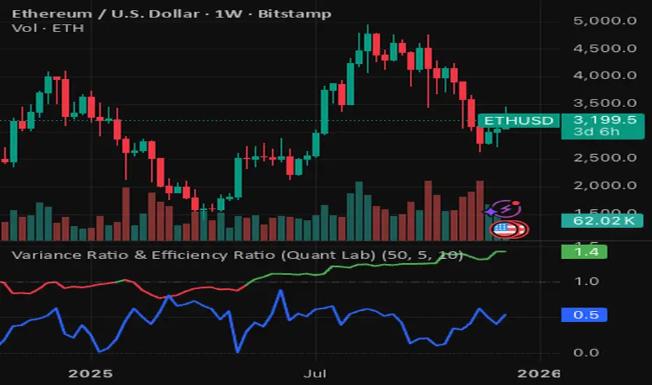
Advanced Multi-Timeframe Trading System (Risk Managed)Description:
This strategy is an original approach that combines two main analytical components to identify potential trade opportunities while simulating realistic trading conditions:
1. Market Trend Analysis via an Approximate Hurst Exponent
• What It Does:
The strategy computes a rough measure of market trending using an approximate Hurst exponent. A value above 0.5 suggests persistent, trending behavior, while a value below 0.5 indicates a tendency toward mean-reversion.
• How It’s Used:
The Hurst exponent is calculated on both the chart’s current timeframe and a higher timeframe (default: Daily) to capture both local and broader market dynamics.
2. Fibonacci Retracement Levels
• What It Does:
Using daily high and low data from a selected timeframe (default: Daily), the script computes key Fibonacci retracement levels.
• How It’s Used:
• The 61.8% level (Golden Ratio) serves as a key threshold:
• A long entry is signaled when the price crosses above this level if the daily Hurst exponent confirms a trending market.
• The 38.2% level is used to identify short-entry opportunities when the price crosses below it and the daily Hurst indicates non-trending conditions.
Signal Logic:
• Long Entry:
When the price crosses above the 61.8% Fibonacci level (Golden Ratio) and the daily Hurst exponent is greater than 0.5, suggesting a trending market.
• Short Entry:
When the price crosses below the 38.2% Fibonacci level and the daily Hurst exponent is less than 0.5, indicating a less trending or potentially reversing market.
Risk Management & Trade Execution:
• Stop-Loss:
Each trade is risk-managed with a stop-loss set at 2% below (for longs) or above (for shorts) the entry price. This ensures that no single trade risks more than a small, sustainable portion of the account.
• Take Profit:
A take profit order targets a risk-reward ratio of 1:2 (i.e., the target profit is twice the amount risked).
• Position Sizing:
Trades are executed with a fixed position size equal to 10% of account equity.
• Trade Frequency Limits:
• Daily Limit: A maximum of 5 trades per day
• Overall Limit: No more than 510 trades during the backtesting period (e.g., since 2019)
These limits are imposed to simulate realistic trading frequency and to avoid overtrading in backtest results.
Backtesting Parameters:
• Initial Capital: $10,000
• Commission: 0.1% per trade
• Slippage: 1 tick per bar
These settings aim to reflect the conditions faced by the average trader and help ensure that the backtesting results are realistic and not misleading.
Chart Overlays & Visual Aids:
• Fibonacci Levels:
The key Fibonacci retracement levels are plotted on the chart, and the zone between the 61.8% and 38.2% levels is highlighted to show a key retracement area.
• Market Trend Background:
The chart background is tinted green when the daily Hurst exponent indicates a trending market (value > 0.5) and red otherwise.
• Information Table:
An on-chart table displays key parameters such as the current Hurst exponent, daily Hurst value, the number of trades executed today, and the global trade count.
Disclaimer:
Past performance is not indicative of future results. This strategy is experimental and provided solely for educational purposes. It is essential that you backtest and paper trade using your own settings before considering any live deployment. The Hurst exponent calculation is an approximation and should be interpreted as a rough gauge of market behavior. Adjust the parameters and risk management settings according to your personal risk tolerance and market conditions.
Additional Notes:
• Originality & Usefulness:
This script is an original mashup that combines trend analysis with Fibonacci retracement methods. The description above explains how these components work together to provide trading signals.
• Realistic Results:
The strategy uses realistic account sizes, commission rates, slippage, and risk management rules to generate backtesting results that are representative of real-world trading.
• Educational Purpose:
This script is intended to support the TradingView community by offering insights into combining multiple analysis techniques in one strategy. It is not a “get-rich-quick” system but rather an educational tool to help traders understand risk management and trade signal logic.
By using this script, you acknowledge that trading involves risk and that you are responsible for testing and adjusting the strategy to fit your own trading environment. This publication is fully open source, and any modifications should include proper attribution if significant portions of the code are reused.
In den Scripts nach "GOLD" suchen
Twitter Model ICT [TradingFinder] MMXM ERL D + FVG + M15 MSS/SMT🔵 Introduction
The Twitter Model ICT is a trading approach based on ICT (Inner Circle Trader) models, focusing on price movement between external and internal liquidity in lower timeframes. This model integrates key concepts such as Market Structure Shift (MSS), Smart Money Technique (SMT) divergence, and CISD level break to identify precise entry points in the market.
The primary goal of this model is to determine key liquidity levels, such as the previous day’s high and low (PDH/PDL) and align them with the Fair Value Gap (FVG) in the 1-hour timeframe. The overall strategy involves framing trades around the 1H FVG and using the M15 Market Structure Shift (MSS) for entry confirmation.
The Twitter Model ICT is designed to utilize external liquidity levels, such as PDH/PDL, as key entry zones. The model identifies FVG in the 1-hour timeframe, which acts as a magnet for price movement. Additionally, traders confirm entries using M15 Market Structure Shift (MSS) and SMT divergence.
Bullish Twitter Model :
In a bullish setup, the price sweeps the previous day’s low (PDL), and after confirming reversal signals, buys are executed in internal liquidity zones. Conversely, in a bearish setup, the price sweeps the previous day’s high (PDH), and after confirming weakness signals, sells are executed.
Bearish Twitter Model :
In short setups, entries are only executed above the Midnight Open, while in long setups, entries are taken below the Midnight Open. Adhering to these principles allows traders to define precise entry and exit points and analyze price movement with greater accuracy based on liquidity and market structure.
🔵 How to Use
The Twitter Model ICT is a liquidity-based trading strategy that analyzes price movements relative to the previous day’s high and low (PDH/PDL) and Fair Value Gap (FVG). This model is applicable in both bullish and bearish directions and utilizes the 1-hour (1H) and 15-minute (M15) timeframes for entry confirmation.
The price first sweeps an external liquidity level (PDH or PDL) and then provides an entry opportunity based on Market Structure Shift (MSS) and SMT divergence. Additionally, the entry should be positioned relative to the Midnight Open, meaning long entries should occur below the Midnight Open and short entries above it.
🟣 Bullish Twitter Model
In a bullish setup, the price first sweeps the previous day’s low (PDL) and reaches an external liquidity level. Then, in the 1-hour timeframe (1H), a bullish Fair Value Gap (FVG) forms, which serves as the price target.
To confirm the entry, a Market Structure Shift (MSS) in the 15-minute timeframe (M15) should be observed, signaling a trend reversal to the upside. Additionally, SMT divergence with correlated assets can indicate weakness in selling pressure.
Under these conditions, a long position is taken below the Midnight Open, with a stop-loss placed at the lowest point of the recent bearish move. The price target for this trade is the FVG in the 1-hour timeframe.
🟣 Bearish Twitter Model
In a bearish setup, the price first sweeps the previous day’s high (PDH) and reaches an external liquidity level. Then, in the 1-hour timeframe (1H), a bearish Fair Value Gap (FVG) is identified, serving as the trade target.
To confirm entry, a Market Structure Shift (MSS) in the 15-minute timeframe (M15) should form, signaling a trend shift to the downside. If an SMT divergence is present, it can provide additional confirmation for the trade.
Once these conditions are met, a short position is taken above the Midnight Open, with a stop-loss placed at the highest level of the recent bullish move. The trade's price target is the FVG in the 1-hour timeframe.
🔵 Settings
Bar Back Check : Determining the return of candles to identify the CISD level.
CISD Level Validity : CISD level validity period based on the number of candles.
Daily Position : Determines whether only the first signal of the day is considered or if signals are evaluated throughout the entire day.
Session : Specifies in which trading sessions the indicator will be active.
Second Symbol : This setting allows you to select another asset for comparison with the primary asset. By default, "XAUUSD" (Gold) is set as the second symbol, but you can change it to any currency pair, stock, or cryptocurrency. For example, you can choose currency pairs like EUR/USD or GBP/USD to identify divergences between these two assets.
Divergence Fractal Periods : This parameter defines the number of past candles to consider when identifying divergences. The default value is 2, but you can change it to suit your preferences. This setting allows you to detect divergences more accurately by selecting a greater number of candles.
The indicator allows displaying sessions based on various time zones. The user can select one of the following options :
UTC (Coordinated Universal Time)
Local Time of the Session
User’s Local Time
Show Open Price : Displays the New York market opening price.
Show PDH / PDL : Displays the previous day’s high and low to identify potential entry points.
Show SMT Divergence : Displays lines and labels for bullish ("+SMT") and bearish ("-SMT") divergences.
🔵 Conclusion
The Twitter Model ICT is an effective approach for analyzing and executing trades in financial markets, utilizing a combination of liquidity principles, market structure, and SMT confirmations to identify optimal entry and exit points.
By analyzing the previous day’s high and low (PDH/PDL), Fair Value Gaps (FVG), and Market Structure Shift (MSS) in the 1H and M15 timeframes, traders can pinpoint liquidity-driven trade opportunities. Additionally, considering the Midnight Open level helps traders avoid random entries and ensures better trade placement.
By applying this model, traders can interpret market movements based on liquidity flow and structural changes, allowing them to fine-tune their trading decisions with higher precision. Ultimately, the Twitter Model ICT provides a structured and logical approach for traders who seek to trade based on liquidity behavior and trend shifts in the market.
Advanced Trend and Volatility Indicator with Alerts by ZaimonThis script presents a comprehensive analytical tool that integrates multiple technical indicators to provide a holistic view of market trends and volatility. By uniquely combining Moving Averages (MA), Relative Strength Index (RSI), Stochastic Oscillator, Bollinger Bands, and Average True Range (ATR), it offers nuanced insights into price movements and helps identify potential trading opportunities.
---
### **Key Features and Integration:**
1. **Moving Averages (MA20 & MA50):**
- **Trend Identification:**
- **Methodology:** Calculates two Simple Moving Averages—MA20 (short-term) and MA50 (long-term).
- **Bullish Trend:** When MA20 crosses above MA50, indicating upward momentum.
- **Bearish Trend:** When MA20 crosses below MA50, signaling downward momentum.
- **Golden Cross & Death Cross Alerts:**
- **Golden Cross:** MA20 crossing above MA50 generates a bullish alert and visual symbol.
- **Death Cross:** MA20 crossing below MA50 triggers a bearish alert and visual symbol.
- **Integration:**
- Serves as the foundational trend indicator, influencing interpretations of other indicators within the script.
2. **Relative Strength Index (RSI):**
- **Momentum Measurement:**
- **Methodology:** Calculates RSI to assess the speed and change of price movements over a 14-period length.
- **Overbought/Oversold Conditions:** Customizable thresholds set at 70 (overbought) and 30 (oversold).
- **Alerts:**
- Generates alerts when RSI crosses above or below the specified thresholds.
- **Integration:**
- Confirms trend strength identified by MAs.
- Overbought/Oversold signals can precede potential trend reversals, especially when aligned with MA crossovers.
3. **Stochastic Oscillator:**
- **Momentum and Reversal Signals:**
- **Methodology:** Uses %K and %D lines to evaluate price momentum relative to high-low range over recent periods.
- **Bullish Signal:** %K crossing above %D in oversold territory (below 20).
- **Bearish Signal:** %K crossing below %D in overbought territory (above 80).
- **Alerts:**
- Provides alerts on bullish and bearish crossovers in extreme regions.
- **Integration:**
- Enhances RSI signals by providing additional momentum confirmation.
- When both RSI and Stochastic indicate overbought/oversold conditions, it strengthens the likelihood of a reversal.
4. **Bollinger Bands:**
- **Volatility Visualization:**
- **Methodology:** Plots upper and lower bands based on standard deviations from a moving average (BB Basis).
- **Dynamic Support/Resistance:** Prices touching or exceeding the bands may indicate potential reversals.
- **Integration:**
- Works with RSI and Stochastic to identify overextended price movements.
- Helps in assessing volatility alongside trend and momentum indicators.
5. **Average True Range (ATR):**
- **Volatility Assessment:**
- **Methodology:** Calculates ATR over a 14-period length to measure market volatility.
- **ATR Bands:** Plots upper and lower bands relative to the current price using an ATR multiplier.
- **Integration:**
- Assists in setting stop-loss and take-profit levels based on current volatility.
- Complements Bollinger Bands for a comprehensive volatility analysis.
6. **Information Table:**
- **Real-Time Data Display:**
- Shows current values of MA20, MA50, RSI, Stochastic %K and %D, BB Basis, ATR, and Trend Status.
- **Trend Status Indicator:**
- Displays "Bullish," "Bearish," or "Sideways" based on MA conditions.
- **Integration:**
- Provides a consolidated view for quick decision-making without analyzing individual indicators separately.
7. **Periodic Labels:**
- **Enhanced Visibility:**
- Adds labels every 50 bars showing RSI and Stochastic values.
- **Integration:**
- Helps track momentum changes over time and spot longer-term patterns.
---
### **How the Components Work Together:**
- **Synergistic Analysis:**
- **Trend Confirmation:** MA crossovers establish the primary trend, while RSI and Stochastic confirm momentum within that trend.
- **Volatility Context:** Bollinger Bands and ATR provide context on market volatility, refining entry and exit points suggested by trend and momentum indicators.
- **Signal Strength:** Concurrent signals from multiple indicators increase confidence in trading decisions.
---
### **Usage Guidelines:**
1. **Trend Analysis:**
- **Identify Trend Direction:**
- Observe MA20 and MA50 crossovers.
- Refer to the Trend Status in the information table.
- **Confirm with Momentum Indicators:**
- Ensure RSI and Stochastic support the identified trend.
2. **Entry and Exit Points:**
- **Overbought/Oversold Conditions:**
- Look for RSI and Stochastic reaching extreme levels.
- Consider entering positions when oversold in a bullish trend or overbought in a bearish trend.
- **Bollinger Band Interactions:**
- Use price interactions with Bollinger Bands to identify potential reversal zones.
3. **Risk Management:**
- **ATR-Based Levels:**
- Set stop-loss and take-profit levels using ATR bands to account for current volatility.
- **Adjusting to Volatility:**
- Modify position sizes and targets based on Bollinger Band width and ATR values.
4. **Alerts Setup:**
- **Customize Alert Thresholds:**
- Configure alerts for MA crossovers, RSI levels, and Stochastic crossovers according to your trading strategy.
- **Stay Informed:**
- Use alerts to monitor key events without constant chart observation.
---
### **Customization:**
- **Flexible Parameters:**
- All indicator lengths, thresholds, and settings are adjustable to suit different trading styles and timeframes.
- **Adjustable Visuals:**
- Modify plot colors, line styles, and label positions to enhance chart readability.
---
### **Originality and Value Addition:**
This script differentiates itself by:
- **Integrated Approach:**
- Seamlessly combining multiple indicators to provide a more comprehensive analysis than using each indicator separately.
- **Enhanced Visualization:**
- Utilizing plots, fills, labels, and an information table to present data intuitively.
- **User-Friendly Features:**
- Pre-configured alerts and real-time data displays reduce the need for manual monitoring.
By explaining how each component interacts and contributes to the overall analysis, the script adds substantial value to traders seeking a multi-faceted tool for market analysis.
---
### **Additional Notes:**
- **Learning Resource:**
- The script is well-commented, serving as an educational tool for those learning Pine Script and technical analysis integration.
- **Further Enhancements:**
- Opportunities exist to incorporate additional indicators like MACD or ADX, and to develop advanced alert logic, such as RSI or Stochastic divergences.
---
### **Disclaimer:**
- **Educational Purpose Only:**
- This script is provided for informational purposes and should not be construed as financial advice.
- **Risk Acknowledgment:**
- Trading involves significant risk; past performance is not indicative of future results.
- **Due Diligence:**
- Users should conduct their own analysis and consider consulting a financial professional before making trading decisions.
---
By providing detailed explanations of the methodologies and the synergistic use of multiple indicators, this script aligns with TradingView's guidelines for originality and usefulness. It offers traders a unique tool that enhances market analysis through the thoughtful integration of technical indicators.
Global M2 Index Percentage### **Global M2 Index Percentage**
**Description:**
The **Global M2 Index Percentage** is a custom indicator designed to track and visualize the global money supply (M2) in a normalized percentage format. It aggregates M2 data from major economies (e.g., the US, EU, China, Japan, and the UK) and adjusts for exchange rates to provide a comprehensive view of global liquidity. This indicator helps traders and investors understand the broader macroeconomic environment, identify trends in money supply, and make informed decisions based on global liquidity conditions.
---
### **How It Works:**
1. **Data Aggregation**:
- The indicator collects M2 data from key economies and adjusts it using exchange rates to calculate a global M2 value.
- The formula for global M2 is:
\
2. **Normalization**:
- The global M2 value is normalized into a percentage (0% to 100%) based on its range over a user-defined period (default: 13 weeks).
- The formula for normalization is:
\
3. **Visualization**:
- The indicator plots the M2 Index as a line chart.
- Key reference levels are highlighted:
- **10% (Red Line)**: Oversold level (low liquidity).
- **50% (Black Line)**: Neutral level.
- **80% (Green Line)**: Overbought level (high liquidity).
---
### **How to Use the Indicator:**
#### **1. Understanding the M2 Index:**
- **Below 10%**: Indicates extremely low liquidity, which may signal economic contraction or tight monetary policy.
- **Above 80%**: Indicates high liquidity, which may signal loose monetary policy or potential inflationary pressures.
- **Between 10% and 80%**: Represents a neutral to moderate liquidity environment.
#### **2. Trading Strategies:**
- **Long-Term Investing**:
- Use the M2 Index to assess global liquidity trends.
- **High M2 Index (e.g., >80%)**: Consider investing in risk assets (stocks, commodities) as liquidity supports growth.
- **Low M2 Index (e.g., <10%)**: Shift to defensive assets (bonds, gold) as liquidity tightens.
- **Short-Term Trading**:
- Combine the M2 Index with technical indicators (e.g., RSI, MACD) for timing entries and exits.
- **M2 Index Rising + RSI Oversold**: Potential buying opportunity.
- **M2 Index Falling + RSI Overbought**: Potential selling opportunity.
#### **3. Macroeconomic Analysis**:
- Use the M2 Index to monitor the impact of central bank policies (e.g., quantitative easing, rate hikes).
- Correlate the M2 Index with inflation data (CPI, PPI) to anticipate inflationary or deflationary trends.
---
### **Key Features:**
- **Customizable Timeframe**: Adjust the lookback period (e.g., 13 weeks, 26 weeks) to suit your trading style.
- **Multi-Economy Data**: Aggregates M2 data from the US, EU, China, Japan, and the UK for a global perspective.
- **Normalized Output**: Converts raw M2 data into an easy-to-interpret percentage format.
- **Reference Levels**: Includes key levels (10%, 50%, 80%) for quick analysis.
---
### **Example Use Case:**
- **Scenario**: The M2 Index rises from 49% to 62% over two weeks.
- **Interpretation**: Global liquidity is increasing, potentially due to central bank stimulus.
- **Action**:
- **Long-Term**: Increase exposure to equities and commodities.
- **Short-Term**: Look for buying opportunities in oversold assets (e.g., RSI < 30).
---
### **Why Use the Global M2 Index Percentage?**
- **Macro Insights**: Understand the broader economic environment and its impact on financial markets.
- **Risk Management**: Identify periods of high or low liquidity to adjust your portfolio accordingly.
- **Enhanced Timing**: Combine with technical analysis for better entry and exit points.
---
### **Conclusion:**
The **Global M2 Index Percentage** is a powerful tool for traders and investors seeking to incorporate macroeconomic data into their strategies. By tracking global liquidity trends, this indicator helps you make informed decisions, whether you're trading short-term or planning long-term investments. Add it to your TradingView charts today and gain a deeper understanding of the global money supply!
---
**Disclaimer**: This indicator is for informational purposes only and should not be considered financial advice. Always conduct your own research and consult with a professional before making investment decisions.
Price Imbalance as Consecutive Levels of AveragesOverview
The Price Imbalance as Consecutive Levels of Averages indicator is an advanced technical analysis tool designed to identify and visualize price imbalances in financial markets. Unlike traditional moving average (MA) indicators that update continuously with each new price bar, this indicator employs moving averages calculated over consecutive, non-overlapping historical windows. This unique approach leverages comparative historical data to provide deeper insights into trend strength and potential reversals, offering traders a more nuanced understanding of market dynamics and reducing the likelihood of false signals or fakeouts.
Key Features
Consecutive Rolling Moving Averages: Utilizes three distinct simple moving averages (SMAs) calculated over consecutive, non-overlapping windows to capture different historical segments of price data.
Dynamic Color-Coded Visualization: SMA lines change color and style based on the relationship between the averages, highlighting both extreme and normal market conditions.
Median and Secondary Median Lines: Provides additional layers of price distribution insight during normal trend conditions through the plotting of primary and secondary median lines.
Fakeout Prevention: Filters out short-term volatility and sharp price movements by requiring consistent historical alignment of multiple moving averages.
Customizable Parameters: Offers flexibility to adjust SMA window lengths and line extensions to align with various trading strategies and timeframes.
Real-Time Updates with Historical Context: Continuously recalculates and updates SMA lines based on comparative historical windows, ensuring that the indicator reflects both current and past market conditions.
Inputs & Settings
Rolling Window Lengths:
Window 1 Length (Most Recent) Bars: Number of bars used to calculate the most recent SMA. (Default: 5, Range: 2–300)
Window 2 Length (Preceding) Bars: Number of bars for the second SMA, shifted by Window 1. (Default: 8, Range: 2–300)
Window 3 Length (Third Rolling) Bars: Number of bars for the third SMA, shifted by the combined lengths of Window 1 and Window 2. (Default: 13, Range: 2–300)
Horizontal Line Extension:
Horizontal Line Extension (Bars): Determines how far each SMA line extends horizontally on the chart. (Default: 10 bars, Range: 1–100)
Functionality and Theory
1. Calculating Consecutive Simple Moving Averages (SMAs):
The indicator calculates three SMAs, each based on distinct and consecutive historical windows of price data. This approach contrasts with traditional MAs that continuously update with each new price bar, offering a static view of past trends rather than an ongoing one.
Mean1 (SMA1): Calculated over the most recent Window 1 Length bars. Represents the short-term trend.
Mean1=∑i=1N1CloseiN1
Mean1=N1∑i=1N1Closei
Where N1N1 is the length of Window 1.
Mean2 (SMA2): Calculated over the preceding Window 2 Length bars, shifted back by Window 1 Length bars. Represents the medium-term trend.
\text{Mean2} = \frac{\sum_{i=1}^{N_2} \text{Close}_{i + N_1}}}{N_2}
Where N2N2 is the length of Window 2.
Mean3 (SMA3): Calculated over the third rolling Window 3 Length bars, shifted back by the combined lengths of Window 1 and Window 2 bars. Represents the long-term trend.
\text{Mean3} = \frac{\sum_{i=1}^{N_3} \text{Close}_{i + N_1 + N_2}}}{N_3}
Where N3N3 is the length of Window 3.
2. Determining Market Conditions:
The relationship between the three SMAs categorizes the market condition into either extreme or normal states, enabling traders to quickly assess trend strength and potential reversals.
Extreme Bullish:
Mean3Mean2>Mean1
Mean3>Mean2>Mean1
Indicates a strong and sustained downward trend. SMA lines are colored purple and styled as dashed lines.
Normal Bullish:
Mean1>Mean2andnot in extreme bullish condition
Indicates a standard upward trend. SMA lines are colored green and styled as solid lines.
Normal Bearish:
Mean1Mean2>Mean1
Mean3>Mean2>Mean1
Normal Bullish:
Mean1>Mean2andnot in Extreme Bullish
Normal Bearish:
Mean1 Mean2 > Mean3
Visualization: All three SMAs are displayed as gold dashed lines.
Median Lines: Not displayed to maintain chart clarity.
Interpretation: Indicates a strong and sustained upward trend. Traders may consider entering long positions, confident in the trend's strength without the distraction of additional lines.
2. Normal Bullish Condition:
SMAs Alignment: Mean1 > Mean2 (not in extreme condition)
Visualization: Mean1 and Mean2 are green solid lines; Mean3 is gray.
Median Lines: A thin blue dotted median line is plotted between Mean1 and Mean2, with two additional thin blue dashed lines as secondary medians.
Interpretation: Confirms an upward trend while providing deeper insights into price distribution. Traders can use the median and secondary median lines to identify optimal entry points and manage risk more effectively.
3. Extreme Bearish Condition:
SMAs Alignment: Mean3 > Mean2 > Mean1
Visualization: All three SMAs are displayed as purple dashed lines.
Median Lines: Not displayed to maintain chart clarity.
Interpretation: Indicates a strong and sustained downward trend. Traders may consider entering short positions, confident in the trend's strength without the distraction of additional lines.
4. Normal Bearish Condition:
SMAs Alignment: Mean1 < Mean2 (not in extreme condition)
Visualization: Mean1 and Mean2 are red solid lines; Mean3 is gray.
Median Lines: A thin blue dotted median line is plotted between Mean1 and Mean2, with two additional thin blue dashed lines as secondary medians.
Interpretation: Confirms a downward trend while providing deeper insights into price distribution. Traders can use the median and secondary median lines to identify optimal entry points and manage risk more effectively.
Customization and Flexibility
The Price Imbalance as Consecutive Levels of Averages indicator is highly adaptable, allowing traders to tailor it to their specific trading styles and market conditions through adjustable parameters:
SMA Window Lengths: Modify the lengths of Window 1, Window 2, and Window 3 to capture different historical trend segments, whether focusing on short-term fluctuations or long-term movements.
Line Extension: Adjust the horizontal extension of SMA and median lines to align with different trading horizons and chart preferences.
Color and Style Preferences: While default colors and styles are optimized for clarity, traders can customize these elements to match their personal chart aesthetics and enhance visual differentiation.
This flexibility ensures that the indicator remains versatile and applicable across various markets, asset classes, and trading strategies, providing valuable insights tailored to individual trading needs.
Conclusion
The Price Imbalance as Consecutive Levels of Averages indicator offers a comprehensive and innovative approach to analyzing price trends and imbalances within financial markets. By utilizing three consecutive, non-overlapping SMAs and incorporating median lines during normal trend conditions, the indicator provides clear and actionable insights into trend strength and price distribution. Its unique design leverages comparative historical data, distinguishing it from traditional moving averages and enhancing its utility in identifying genuine market movements while minimizing false signals. This dynamic and customizable tool empowers traders to refine their technical analysis, optimize their trading strategies, and navigate the markets with greater confidence and precision.
Geo. Geo.
This library provides a comprehensive set of geometric functions based on 2 simple types for point and line manipulation, point array calculations, some vector operations (Borrowed from @ricardosantos ), angle calculations, and basic polygon analysis. It offers tools for creating, transforming, and analyzing geometric shapes and their relationships.
View the source code for detailed documentation on each function and type.
═════════════════════════════════════════════════════════════════════════
█ OVERVIEW
This library enhances TradingView's Pine Script with robust geometric capabilities. It introduces the Point and Line types, along with a suite of functions for various geometric operations. These functionalities empower you to perform advanced calculations, manipulations, and analyses involving points, lines, vectors, angles, and polygons directly within your Pine scripts. The example is at the bottom of the script. ( Commented out )
█ CONCEPTS
This library revolves around two fundamental types:
• Point: Represents a point in 2D space with x and y coordinates, along with optional 'a' (angle) and 'v' (value) fields for versatile use. Crucially, for plotting, utilize the `.to_chart_point()` method to convert Points into plottable chart.point objects.
• Line: Defined by a starting Point and a slope , enabling calculations like getting y for a given x, or finding intersection points.
█ FEATURES
• Point Manipulation: Perform operations like addition, subtraction, scaling, rotation, normalization, calculating distances, dot products, cross products, midpoints, and more with Point objects.
• Line Operations: Create lines, determine their slope, calculate y from x (and vice versa), and find the intersection points of two lines.
• Vector Operations: Perform vector addition, subtraction, multiplication, division, negation, perpendicular vector calculation, floor, fractional part, sine, absolute value, modulus, sign, round, scaling, rescaling, rotation, and ceiling operations.
• Angle Calculations: Compute angles between points in degrees or radians, including signed, unsigned, and 360-degree angles.
• Polygon Analysis: Calculate the area, perimeter, and centroid of polygons. Check if a point is inside a given polygon and determine the convex hull perimeter.
• Chart Plotting: Conveniently convert Point objects to chart.point objects for plotting lines and points on the chart. The library also includes functions for plotting lines between individual and series of points.
• Utility Functions: Includes helper functions such as square root, square, cosine, sine, tangent, arc cosine, arc sine, arc tangent, atan2, absolute distance, golden ratio tolerance check, fractional part, and safe index/check for chart plotting boundaries.
█ HOW TO USE
1 — Include the library in your script using:
import kaigouthro/geo/1
2 — Create Point and Line objects:
p1 = geo.Point(bar_index, close)
p2 = geo.Point(bar_index , open)
myLine = geo.Line(p1, geo.slope(p1, p2))
// maybe use that line to detect a crossing for an alert ... hmmm
3 — Utilize the provided functions:
distance = geo.distance(p1, p2)
intersection = geo.intersection(line1, line2)
4 — For plotting labels, lines, convert Point to chart.point :
label.new(p1.to_chart_point(), " Hi ")
line.new(p1.to_chart_point(),p2.to_chart_point())
█ NOTES
This description provides a concise overview. Consult the library's source code for in-depth documentation, including detailed descriptions, parameter types, and return values for each function and method. The source code is structured with comprehensive comments using the `//@` format for seamless integration with TradingView's auto-documentation features.
█ Possibilities..
Library "geo"
This library provides a comprehensive set of geometric functions and types, including point and line manipulation, vector operations, angle calculations, and polygon analysis. It offers tools for creating, transforming, and analyzing geometric shapes and their relationships.
sqrt(value)
Square root function
Parameters:
value (float) : (float) - The number to take the square root of
Returns: (float) - The square root of the input value
sqr(x)
Square function
Parameters:
x (float) : (float) - The number to square
Returns: (float) - The square of the input value
cos(v)
Cosine function
Parameters:
v (float) : (series float) - The value to find the cosine of
Returns: (series float) - The cosine of the input value
sin(v)
Sine function
Parameters:
v (float) : (series float) - The value to find the sine of
Returns: (series float) - The sine of the input value
tan(v)
Tangent function
Parameters:
v (float) : (series float) - The value to find the tangent of
Returns: (series float) - The tangent of the input value
acos(v)
Arc cosine function
Parameters:
v (float) : (series float) - The value to find the arc cosine of
Returns: (series float) - The arc cosine of the input value
asin(v)
Arc sine function
Parameters:
v (float) : (series float) - The value to find the arc sine of
Returns: (series float) - The arc sine of the input value
atan(v)
Arc tangent function
Parameters:
v (float) : (series float) - The value to find the arc tangent of
Returns: (series float) - The arc tangent of the input value
atan2(dy, dx)
atan2 function
Parameters:
dy (float) : (float) - The y-coordinate
dx (float) : (float) - The x-coordinate
Returns: (float) - The angle in radians
gap(_value1, __value2)
Absolute distance between any two float values
Parameters:
_value1 (float) : First value
__value2 (float)
Returns: Absolute Positive Distance
phi_tol(a, b, tolerance)
Check if the ratio is within the tolerance of the golden ratio
Parameters:
a (float) : (float) The first number
b (float) : (float) The second number
tolerance (float) : (float) The tolerance percennt as 1 = 1 percent
Returns: (bool) True if the ratio is within the tolerance, false otherwise
frac(x)
frad Fractional
Parameters:
x (float) : (float) - The number to convert to fractional
Returns: (float) - The number converted to fractional
safeindex(x, limit)
limiting int to hold the value within the chart range
Parameters:
x (float) : (float) - The number to limit
limit (int)
Returns: (int) - The number limited to the chart range
safecheck(x, limit)
limiting int check if within the chartplottable range
Parameters:
x (float) : (float) - The number to limit
limit (int)
Returns: (int) - The number limited to the chart range
interpolate(a, b, t)
interpolate between two values
Parameters:
a (float) : (float) - The first value
b (float) : (float) - The second value
t (float) : (float) - The interpolation factor (0 to 1)
Returns: (float) - The interpolated value
gcd(_numerator, _denominator)
Greatest common divisor of two integers
Parameters:
_numerator (int)
_denominator (int)
Returns: (int) The greatest common divisor
method set_x(self, value)
Set the x value of the point, and pass point for chaining
Namespace types: Point
Parameters:
self (Point) : (Point) The point to modify
value (float) : (float) The new x-coordinate
method set_y(self, value)
Set the y value of the point, and pass point for chaining
Namespace types: Point
Parameters:
self (Point) : (Point) The point to modify
value (float) : (float) The new y-coordinate
method get_x(self)
Get the x value of the point
Namespace types: Point
Parameters:
self (Point) : (Point) The point to get the x-coordinate from
Returns: (float) The x-coordinate
method get_y(self)
Get the y value of the point
Namespace types: Point
Parameters:
self (Point) : (Point) The point to get the y-coordinate from
Returns: (float) The y-coordinate
method vmin(self)
Lowest element of the point
Namespace types: Point
Parameters:
self (Point) : (Point) The point
Returns: (float) The lowest value between x and y
method vmax(self)
Highest element of the point
Namespace types: Point
Parameters:
self (Point) : (Point) The point
Returns: (float) The highest value between x and y
method add(p1, p2)
Addition
Namespace types: Point
Parameters:
p1 (Point) : (Point) - The first point
p2 (Point) : (Point) - The second point
Returns: (Point) - the add of the two points
method sub(p1, p2)
Subtraction
Namespace types: Point
Parameters:
p1 (Point) : (Point) - The first point
p2 (Point) : (Point) - The second point
Returns: (Point) - the sub of the two points
method mul(p, scalar)
Multiplication by scalar
Namespace types: Point
Parameters:
p (Point) : (Point) - The point
scalar (float) : (float) - The scalar to multiply by
Returns: (Point) - the multiplied point of the point and the scalar
method div(p, scalar)
Division by scalar
Namespace types: Point
Parameters:
p (Point) : (Point) - The point
scalar (float) : (float) - The scalar to divide by
Returns: (Point) - the divided point of the point and the scalar
method rotate(p, angle)
Rotate a point around the origin by an angle (in degrees)
Namespace types: Point
Parameters:
p (Point) : (Point) - The point to rotate
angle (float) : (float) - The angle to rotate by in degrees
Returns: (Point) - the rotated point
method length(p)
Length of the vector from origin to the point
Namespace types: Point
Parameters:
p (Point) : (Point) - The point
Returns: (float) - the length of the point
method length_squared(p)
Length squared of the vector
Namespace types: Point
Parameters:
p (Point) : (Point) The point
Returns: (float) The squared length of the point
method normalize(p)
Normalize the point to a unit vector
Namespace types: Point
Parameters:
p (Point) : (Point) - The point to normalize
Returns: (Point) - the normalized point
method dot(p1, p2)
Dot product
Namespace types: Point
Parameters:
p1 (Point) : (Point) - The first point
p2 (Point) : (Point) - The second point
Returns: (float) - the dot of the two points
method cross(p1, p2)
Cross product result (in 2D, this is a scalar)
Namespace types: Point
Parameters:
p1 (Point) : (Point) - The first point
p2 (Point) : (Point) - The second point
Returns: (float) - the cross of the two points
method distance(p1, p2)
Distance between two points
Namespace types: Point
Parameters:
p1 (Point) : (Point) - The first point
p2 (Point) : (Point) - The second point
Returns: (float) - the distance of the two points
method Point(x, y, a, v)
Point Create Convenience
Namespace types: series float, simple float, input float, const float
Parameters:
x (float)
y (float)
a (float)
v (float)
Returns: (Point) new point
method angle(p1, p2)
Angle between two points in degrees
Namespace types: Point
Parameters:
p1 (Point) : (Point) - The first point
p2 (Point) : (Point) - The second point
Returns: (float) - the angle of the first point and the second point
method angle_between(p, pivot, other)
Angle between two points in degrees from a pivot point
Namespace types: Point
Parameters:
p (Point) : (Point) - The point to calculate the angle from
pivot (Point) : (Point) - The pivot point
other (Point) : (Point) - The other point
Returns: (float) - the angle between the two points
method translate(p, from_origin, to_origin)
Translate a point from one origin to another
Namespace types: Point
Parameters:
p (Point) : (Point) - The point to translate
from_origin (Point) : (Point) - The origin to translate from
to_origin (Point) : (Point) - The origin to translate to
Returns: (Point) - the translated point
method midpoint(p1, p2)
Midpoint of two points
Namespace types: Point
Parameters:
p1 (Point) : (Point) - The first point
p2 (Point) : (Point) - The second point
Returns: (Point) - The midpoint of the two points
method rotate_around(p, angle, pivot)
Rotate a point around a pivot point by an angle (in degrees)
Namespace types: Point
Parameters:
p (Point) : (Point) - The point to rotate
angle (float) : (float) - The angle to rotate by in degrees
pivot (Point) : (Point) - The pivot point to rotate around
Returns: (Point) - the rotated point
method multiply(_a, _b)
Multiply vector _a with _b
Namespace types: Point
Parameters:
_a (Point) : (Point) The first point
_b (Point) : (Point) The second point
Returns: (Point) The result of the multiplication
method divide(_a, _b)
Divide vector _a by _b
Namespace types: Point
Parameters:
_a (Point) : (Point) The first point
_b (Point) : (Point) The second point
Returns: (Point) The result of the division
method negate(_a)
Negative of vector _a
Namespace types: Point
Parameters:
_a (Point) : (Point) The point to negate
Returns: (Point) The negated point
method perp(_a)
Perpendicular Vector of _a
Namespace types: Point
Parameters:
_a (Point) : (Point) The point
Returns: (Point) The perpendicular point
method vfloor(_a)
Compute the floor of argument vector _a
Namespace types: Point
Parameters:
_a (Point) : (Point) The point
Returns: (Point) The floor of the point
method fractional(_a)
Compute the fractional part of the elements from vector _a
Namespace types: Point
Parameters:
_a (Point) : (Point) The point
Returns: (Point) The fractional part of the point
method vsin(_a)
Compute the sine of argument vector _a
Namespace types: Point
Parameters:
_a (Point) : (Point) The point
Returns: (Point) The sine of the point
lcm(a, b)
Least common multiple of two integers
Parameters:
a (int) : (int) The first integer
b (int) : (int) The second integer
Returns: (int) The least common multiple
method vabs(_a)
Compute the absolute of argument vector _a
Namespace types: Point
Parameters:
_a (Point) : (Point) The point
Returns: (Point) The absolute of the point
method vmod(_a, _b)
Compute the mod of argument vector _a
Namespace types: Point
Parameters:
_a (Point) : (Point) The point
_b (float) : (float) The mod
Returns: (Point) The mod of the point
method vsign(_a)
Compute the sign of argument vector _a
Namespace types: Point
Parameters:
_a (Point) : (Point) The point
Returns: (Point) The sign of the point
method vround(_a)
Compute the round of argument vector _a
Namespace types: Point
Parameters:
_a (Point) : (Point) The point
Returns: (Point) The round of the point
method normalize_y(p, height)
normalizes the y value of a point to an input height
Namespace types: Point
Parameters:
p (Point) : (Point) - The point to normalize
height (float) : (float) - The height to normalize to
Returns: (Point) - the normalized point
centroid(points)
Calculate the centroid of multiple points
Parameters:
points (array) : (array) The array of points
Returns: (Point) The centroid point
random_point(_height, _width, _origin, _centered)
Random Point in a given height and width
Parameters:
_height (float) : (float) The height of the area to generate the point in
_width (float) : (float) The width of the area to generate the point in
_origin (Point) : (Point) The origin of the area to generate the point in (default: na, will create a Point(0, 0))
_centered (bool) : (bool) Center the origin point in the area, otherwise, positive h/w (default: false)
Returns: (Point) The random point in the given area
random_point_array(_origin, _height, _width, _centered, _count)
Random Point Array in a given height and width
Parameters:
_origin (Point) : (Point) The origin of the area to generate the array (default: na, will create a Point(0, 0))
_height (float) : (float) The height of the area to generate the array
_width (float) : (float) The width of the area to generate the array
_centered (bool) : (bool) Center the origin point in the area, otherwise, positive h/w (default: false)
_count (int) : (int) The number of points to generate (default: 50)
Returns: (array) The random point array in the given area
method sort_points(points, by_x)
Sorts an array of points by x or y coordinate
Namespace types: array
Parameters:
points (array) : (array) The array of points to sort
by_x (bool) : (bool) Whether to sort by x-coordinate (true) or y-coordinate (false)
Returns: (array) The sorted array of points
method equals(_a, _b)
Compares two points for equality
Namespace types: Point
Parameters:
_a (Point) : (Point) The first point
_b (Point) : (Point) The second point
Returns: (bool) True if the points are equal, false otherwise
method max(origin, _a, _b)
Maximum of two points from origin, using dot product
Namespace types: Point
Parameters:
origin (Point)
_a (Point) : (Point) The first point
_b (Point) : (Point) The second point
Returns: (Point) The maximum point
method min(origin, _a, _b)
Minimum of two points from origin, using dot product
Namespace types: Point
Parameters:
origin (Point)
_a (Point) : (Point) The first point
_b (Point) : (Point) The second point
Returns: (Point) The minimum point
method avg_x(points)
Average x of point array
Namespace types: array
Parameters:
points (array) : (array) The array of points
Returns: (float) The average x-coordinate
method avg_y(points)
Average y of point array
Namespace types: array
Parameters:
points (array) : (array) The array of points
Returns: (float) The average y-coordinate
method range_x(points)
Range of x values in point array
Namespace types: array
Parameters:
points (array) : (array) The array of points
Returns: (float) The range of x-coordinates
method range_y(points)
Range of y values in point array
Namespace types: array
Parameters:
points (array) : (array) The array of points
Returns: (float) The range of y-coordinates
method max_x(points)
max of x values in point array
Namespace types: array
Parameters:
points (array) : (array) The array of points
Returns: (float) The max of x-coordinates
method min_y(points)
min of x values in point array
Namespace types: array
Parameters:
points (array) : (array) The array of points
Returns: (float) The min of x-coordinates
method scale(_a, _scalar)
Scale a point by a scalar
Namespace types: Point
Parameters:
_a (Point) : (Point) The point to scale
_scalar (float) : (float) The scalar value
Returns: (Point) The scaled point
method rescale(_a, _length)
Rescale a point to a new magnitude
Namespace types: Point
Parameters:
_a (Point) : (Point) The point to rescale
_length (float) : (float) The new magnitude
Returns: (Point) The rescaled point
method rotate_rad(_a, _radians)
Rotate a point by an angle in radians
Namespace types: Point
Parameters:
_a (Point) : (Point) The point to rotate
_radians (float) : (float) The angle in radians
Returns: (Point) The rotated point
method rotate_degree(_a, _degree)
Rotate a point by an angle in degrees
Namespace types: Point
Parameters:
_a (Point) : (Point) The point to rotate
_degree (float) : (float) The angle in degrees
Returns: (Point) The rotated point
method vceil(_a, _digits)
Ceil a point to a certain number of digits
Namespace types: Point
Parameters:
_a (Point) : (Point) The point to ceil
_digits (int) : (int) The number of digits to ceil to
Returns: (Point) The ceiled point
method vpow(_a, _exponent)
Raise both point elements to a power
Namespace types: Point
Parameters:
_a (Point) : (Point) The point
_exponent (float) : (float) The exponent
Returns: (Point) The point with elements raised to the power
method perpendicular_distance(_a, _b, _c)
Distance from point _a to line between _b and _c
Namespace types: Point
Parameters:
_a (Point) : (Point) The point
_b (Point) : (Point) The start point of the line
_c (Point) : (Point) The end point of the line
Returns: (float) The perpendicular distance
method project(_a, _axis)
Project a point onto another
Namespace types: Point
Parameters:
_a (Point) : (Point) The point to project
_axis (Point) : (Point) The point to project onto
Returns: (Point) The projected point
method projectN(_a, _axis)
Project a point onto a point of unit length
Namespace types: Point
Parameters:
_a (Point) : (Point) The point to project
_axis (Point) : (Point) The unit length point to project onto
Returns: (Point) The projected point
method reflect(_a, _axis)
Reflect a point on another
Namespace types: Point
Parameters:
_a (Point) : (Point) The point to reflect
_axis (Point) : (Point) The point to reflect on
Returns: (Point) The reflected point
method reflectN(_a, _axis)
Reflect a point to an arbitrary axis
Namespace types: Point
Parameters:
_a (Point) : (Point) The point to reflect
_axis (Point) : (Point) The axis to reflect to
Returns: (Point) The reflected point
method angle_rad(_a)
Angle in radians of a point
Namespace types: Point
Parameters:
_a (Point) : (Point) The point
Returns: (float) The angle in radians
method angle_unsigned(_a, _b)
Unsigned degree angle between 0 and +180 by given two points
Namespace types: Point
Parameters:
_a (Point) : (Point) The first point
_b (Point) : (Point) The second point
Returns: (float) The unsigned angle in degrees
method angle_signed(_a, _b)
Signed degree angle between -180 and +180 by given two points
Namespace types: Point
Parameters:
_a (Point) : (Point) The first point
_b (Point) : (Point) The second point
Returns: (float) The signed angle in degrees
method angle_360(_a, _b)
Degree angle between 0 and 360 by given two points
Namespace types: Point
Parameters:
_a (Point) : (Point) The first point
_b (Point) : (Point) The second point
Returns: (float) The angle in degrees (0-360)
method clamp(_a, _vmin, _vmax)
Restricts a point between a min and max value
Namespace types: Point
Parameters:
_a (Point) : (Point) The point to restrict
_vmin (Point) : (Point) The minimum point
_vmax (Point) : (Point) The maximum point
Returns: (Point) The restricted point
method lerp(_a, _b, _rate_of_move)
Linearly interpolates between points a and b by _rate_of_move
Namespace types: Point
Parameters:
_a (Point) : (Point) The starting point
_b (Point) : (Point) The ending point
_rate_of_move (float) : (float) The rate of movement (0-1)
Returns: (Point) The interpolated point
method slope(p1, p2)
Slope of a line between two points
Namespace types: Point
Parameters:
p1 (Point) : (Point) - The first point
p2 (Point) : (Point) - The second point
Returns: (float) - The slope of the line
method gety(self, x)
Get y-coordinate of a point on the line given its x-coordinate
Namespace types: Line
Parameters:
self (Line) : (Line) - The line
x (float) : (float) - The x-coordinate
Returns: (float) - The y-coordinate
method getx(self, y)
Get x-coordinate of a point on the line given its y-coordinate
Namespace types: Line
Parameters:
self (Line) : (Line) - The line
y (float) : (float) - The y-coordinate
Returns: (float) - The x-coordinate
method intersection(self, other)
Intersection point of two lines
Namespace types: Line
Parameters:
self (Line) : (Line) - The first line
other (Line) : (Line) - The second line
Returns: (Point) - The intersection point
method calculate_arc_point(self, b, p3)
Calculate a point on the arc defined by three points
Namespace types: Point
Parameters:
self (Point) : (Point) The starting point of the arc
b (Point) : (Point) The middle point of the arc
p3 (Point) : (Point) The end point of the arc
Returns: (Point) A point on the arc
approximate_center(point1, point2, point3)
Approximate the center of a spiral using three points
Parameters:
point1 (Point) : (Point) The first point
point2 (Point) : (Point) The second point
point3 (Point) : (Point) The third point
Returns: (Point) The approximate center point
createEdge(center, radius, angle)
Get coordinate from center by radius and angle
Parameters:
center (Point) : (Point) - The center point
radius (float) : (float) - The radius of the circle
angle (float) : (float) - The angle in degrees
Returns: (Point) - The coordinate on the circle
getGrowthFactor(p1, p2, p3)
Get growth factor of spiral point
Parameters:
p1 (Point) : (Point) - The first point
p2 (Point) : (Point) - The second point
p3 (Point) : (Point) - The third point
Returns: (float) - The growth factor
method to_chart_point(point)
Convert Point to chart.point using chart.point.from_index(safeindex(point.x), point.y)
Namespace types: Point
Parameters:
point (Point) : (Point) - The point to convert
Returns: (chart.point) - The chart.point representation of the input point
method plotline(p1, p2, col, width)
Draw a line from p1 to p2
Namespace types: Point
Parameters:
p1 (Point) : (Point) First point
p2 (Point) : (Point) Second point
col (color)
width (int)
Returns: (line) Line object
method drawlines(points, col, ignore_boundary)
Draw lines between points in an array
Namespace types: array
Parameters:
points (array) : (array) The array of points
col (color) : (color) The color of the lines
ignore_boundary (bool) : (bool) The color of the lines
method to_chart_points(points)
Draw an array of points as chart points on the chart with line.new(chartpoint1, chartpoint2, color=linecolor)
Namespace types: array
Parameters:
points (array) : (array) - The points to draw
Returns: (array) The array of chart points
polygon_area(points)
Calculate the area of a polygon defined by an array of points
Parameters:
points (array) : (array) The array of points representing the polygon vertices
Returns: (float) The area of the polygon
polygon_perimeter(points)
Calculate the perimeter of a polygon
Parameters:
points (array) : (array) Array of points defining the polygon
Returns: (float) Perimeter of the polygon
is_point_in_polygon(point, _polygon)
Check if a point is inside a polygon
Parameters:
point (Point) : (Point) The point to check
_polygon (array)
Returns: (bool) True if the point is inside the polygon, false otherwise
method perimeter(points)
Calculates the convex hull perimeter of a set of points
Namespace types: array
Parameters:
points (array) : (array) The array of points
Returns: (array) The array of points forming the convex hull perimeter
Point
A Point, can be used for vector, floating calcs, etc. Use the cp method for plots
Fields:
x (series float) : (float) The x-coordinate
y (series float) : (float) The y-coordinate
a (series float) : (float) An Angle storage spot
v (series float) : (float) A Value
Line
Line
Fields:
point (Point) : (Point) The starting point of the line
slope (series float) : (float) The slope of the line
GOMTRY.
Doji Double Top & Double Bottom
FUNCTION :
This indicator checks if 2 consecutive candlesticks are formed in such a way that both the lows or both the highs of the consecutive candlesticks are almost at the same level and either of them is a doji
TIMEFRAMES :
it works on daily, weekly, monthly and higher timeframes
CRITERIA :
There is maximum difference value between 2 consecutive candlesticks' lows or 2 consecutive candlesticks' highs
Minimum value of the doji's wick size
Maximum value of the doji's body size
These 3 conditions need to be fulfilled for the 2 consecutive candlesticks to be considered as a Double top or Double bottom by this indicator
EXAMPLES :
Here the indicator is giving only double Bottom signals on CRUDE OIL chart
Here the indicator is giving only double top signals on GOLD chart
Here the indicator gives both double top & double bottom signals on EUR/USD Daily chart
Here the indicator is giving both double top & double bottom signals on EUR/USD Half-Yearly chart
DEFINITIONS :
There are 2 types -
DOJI DOUBLE BOTTOM - if the lows of 2 consecutive candlesticks are almost at the same level & either of them is doji then it is called Double Bottom and market is supposed to go higher after forming it.
DOJI DOUBLE TOP - if the highs of 2 consecutive candlesticks are almost at the same level & either of them is doji then it is called Double Top and market is supposed to go lower after forming it.
SETTINGS :
There are options to change the value of each of the 3 parameters within the indicator's settings for daily, weekly & monthly chart [
LIMITATIONS :
You should not trade based on the signals from this indicator solely, you should check other parameters too before making trading decision
STRX - Correlation DominationThis indicator displays the correlation among three selected assets (for example, Gold, Dollar Index, and Nasdaq) on a custom timeframe. A table positioned at the top-right corner of the chart lets you quickly see the correlation between:
Asset 1 vs Asset 2
Asset 1 vs Asset 3
Asset 2 vs Asset 3
Correlations are calculated using the Pearson correlation function (ta.correlation). If the correlation is greater than or equal to 0.4, the value appears in green (strong positive correlation). If it is less than or equal to -0.4, it appears in red (strong negative correlation). Otherwise, it is displayed in yellow (weak correlation).
Multi-asset and multi-timeframe: Compare up to three instruments at once on your chosen timeframe.
Customizable period: Use the “Correlation Period” setting to adjust the correlation calculation window.
Clear table format: The results are immediately visible in an easy-to-read table.
Disclaimer: This script is provided solely for educational and informational purposes. It does not constitute a recommendation or an invitation to invest. Use it as an additional resource and always conduct thorough market analysis before opening any trading positions. Past performance does not guarantee future results.
CandelaCharts - Swing Failure Pattern (SFP)# SWING FAILURE PATTERN
📝 Overview
The Swing Failure Pattern (SFP) indicator is designed to identify and highlight Swing Failure Patterns on a user’s chart. This pattern typically emerges when significant market participants generate liquidity by driving price action to key levels. An SFP occurs when the price temporarily breaks above a resistance level or below a support level, only to quickly reverse and return within the previous range. These movements are often associated with stop-loss hunting or liquidity grabs, providing traders with potential opportunities to anticipate reversals or key market turning points.
A Bullish SFP occurs when the price dips below a key support level, triggering stop-loss orders, but then swiftly reverses upward, signaling a potential upward trend or reversal.
A Bearish SFP happens when the price spikes above a key resistance level, triggering stop-losses of short positions, but then quickly reverses downward, indicating a potential bearish trend or reversal.
The indicator is a powerful tool for traders, helping to identify liquidity grabs and potential reversal points in real-time. Marking bullish and bearish Swing Failure Patterns on the chart, it provides clear visual cues for spotting market traps set by major players, enabling more informed trading decisions and improved risk management.
📦 Features
Bullish/Bearish SFPs
Styling
⚙️ Settings
Length: Determines the detection length of each SFP
Bullish SFP: Displays the bullish SFPs
Bearish SFP: Displays the bearish SFPs
Label: Controls the size of the label
⚡️ Showcase
Bullish
Bearish
Both
📒 Usage
The best approach is to combine a few complementary indicators to gain a clearer market perspective. This doesn’t mean relying on the Golden Cross, RSI divergences, SFPs, and funding rates simultaneously, but rather focusing on one or two that align well in a given scenario.
The example above demonstrates the confluence of a Bearish Swing Failure Pattern (SFP) with an RSI divergence. This combination strengthens the signal, as the Bearish SFP indicates a potential reversal after a liquidity grab, while the RSI divergence confirms weakening momentum at the key level. Together, these indicators provide a more robust setup for identifying potential market reversals with greater confidence.
🚨 Alerts
This script provides alert options for all signals.
Bearish Signal
A bearish signal is triggered when a Bearish SFP is formed.
Bullish Signal
A bullish signal is triggered when a Bullish SFP is formed.
⚠️ Disclaimer
Trading involves significant risk, and many participants may incur losses. The content on this site is not intended as financial advice and should not be interpreted as such. Decisions to buy, sell, hold, or trade securities, commodities, or other financial instruments carry inherent risks and are best made with guidance from qualified financial professionals. Past performance is not indicative of future results.
4H CRT (1AM and 5AM)This TradingView script is designed to assist traders in implementing the "4-Hour Candle Ranges Theory Strategy (CRT)" by identifying key levels and setups based on the 1am and 4am (5am) 4-hour candles. This strategy is particularly effective for trading high-volatility assets such as Gold, EUR/USD, NAS100, US30, and S&P500, with US30 showing a notably high win rate. Here's how the strategy works:
Key Features:
1. Marking 1am and 4am 4-Hour Candle Ranges
- The script highlights the high and low of the 1am 4-hour candle.
- It visually tracks whether the high or low of the 1am candle is taken out by the subsequent 4-hour candle (5am).
2. Entry Setup Rules
- Primary Setup: Wait for the high or low of the 1am candle to be taken out by the 5am candle. Once this sweep occurs, wait for a Market Structure Shift (MSS) on the lower time frame (15min) to confirm your entry.
- Secondary Setup: If the 5am candle fails to take out the high or low of the 1am candle, the setup focuses on the levels formed by the 5am candle.
3. Trade Execution on 15-Minute Timeframe
- The script supports a lower time frame (15min) view to identify MSS and fine-tune entries.
4. Rinse and Repeat
- This process can be applied daily for consistent opportunities across the specified assets.
Advantages:
- Provides clear visual markers for key levels based on the 4-hour candles.
- Automates level plotting, saving traders time and reducing manual errors.
- Integrates well with the 15-minute timeframe for precise entry triggers.
- Optimized for popular trading instruments, especially US30 for a higher probability of success.
This script simplifies the application of CRT by automating the process of identifying and marking critical levels, enabling traders to focus on executing high-probability setups effectively.
Created by Hamid (poraymanfx)
Fibonacci Channel Standard Deviation levels based off 200MAThis script dynamically combines Fibonacci levels with the 200-period simple moving average (SMA), offering a powerful tool for identifying high-probability support and resistance zones. By adjusting to the changing 200 SMA, the script remains relevant across different market phases.
Key Features:
Dynamic Fibonacci Levels:
The script automatically calculates Fibonacci retracements and extensions relative to the 200 SMA.
These levels adapt to market trends, offering more relevant zones compared to static Fibonacci tools.
Support and Resistance Zones:
In uptrends, price often respects retracement levels above the 200 SMA (e.g., 38.2%, 50%, 61.8%).
In downtrends, price may interact with retracements and extensions below the 200 SMA (e.g., 23.6%, 1.618).
Customizable Confluence Zones:
Key levels such as the golden pocket (61.8%–65%) are highlighted as high-probability zones for reversals or continuations.
Extensions (e.g., 1.618) can serve as profit targets or bearish continuation points.
Practical Applications:
Identifying Reversal Zones:
Look for confluence between Fibonacci levels and the 200 SMA to identify potential reversal points.
Example: A pullback to the 61.8%–65% golden pocket near the 200 SMA often signals a bullish reversal.
Trend Confirmation:
In uptrends, price respecting Fibonacci retracements above the 200 SMA (e.g., 38.2%, 50%) confirms strength.
Use Fibonacci extensions (e.g., 1.618) as profit targets during strong trends.
Dynamic Risk Management:
Place stop-losses just below key Fibonacci retracement levels near the 200 SMA to minimize risk.
Bearish Scenarios:
Below the 200 SMA, Fibonacci retracements and extensions act as resistance levels and bearish targets.
How to Use:
Volume Confirmation: Watch for volume spikes near Fibonacci levels to confirm support or resistance.
Price Action: Combine with candlestick patterns (e.g., engulfing candles, pin bars) for precise entries.
Trend Indicators: Use in conjunction with shorter moving averages or RSI to confirm market direction.
Example Setup:
Scenario: Price retraces to the 61.8% Fibonacci level while holding above the 200 SMA.
Confirmation: Volume spikes, and a bullish engulfing candle forms.
Action: Enter long with a stop-loss just below the 200 SMA and target extensions like 1.618.
Key Takeaways:
The 200 SMA serves as a reliable long-term trend anchor.
Fibonacci retracements and extensions provide dynamic zones for trade entries, exits, and risk management.
Combining this tool with volume, price action, or other indicators enhances its effectiveness.
Volatility IndicatorThe volatility indicator presented here is based on multiple volatility indices that reflect the market’s expectation of future price fluctuations across different asset classes, including equities, commodities, and currencies. These indices serve as valuable tools for traders and analysts seeking to anticipate potential market movements, as volatility is a key factor influencing asset prices and market dynamics (Bollerslev, 1986).
Volatility, defined as the magnitude of price changes, is often regarded as a measure of market uncertainty or risk. Financial markets exhibit periods of heightened volatility that may precede significant price movements, whether upward or downward (Christoffersen, 1998). The indicator presented in this script tracks several key volatility indices, including the VIX (S&P 500), GVZ (Gold), OVX (Crude Oil), and others, to help identify periods of increased uncertainty that could signal potential market turning points.
Volatility Indices and Their Relevance
Volatility indices like the VIX are considered “fear gauges” as they reflect the market’s expectation of future volatility derived from the pricing of options. A rising VIX typically signals increasing investor uncertainty and fear, which often precedes market corrections or significant price movements. In contrast, a falling VIX may suggest complacency or confidence in continued market stability (Whaley, 2000).
The other volatility indices incorporated in the indicator script, such as the GVZ (Gold Volatility Index) and OVX (Oil Volatility Index), capture the market’s perception of volatility in specific asset classes. For instance, GVZ reflects market expectations for volatility in the gold market, which can be influenced by factors such as geopolitical instability, inflation expectations, and changes in investor sentiment toward safe-haven assets. Similarly, OVX tracks the implied volatility of crude oil options, which is a crucial factor for predicting price movements in energy markets, often driven by geopolitical events, OPEC decisions, and supply-demand imbalances (Pindyck, 2004).
Using the Indicator to Identify Market Movements
The volatility indicator alerts traders when specific volatility indices exceed a defined threshold, which may signal a change in market sentiment or an upcoming price movement. These thresholds, set by the user, are typically based on historical levels of volatility that have preceded significant market changes. When a volatility index exceeds this threshold, it suggests that market participants expect greater uncertainty, which often correlates with increased price volatility and the possibility of a trend reversal.
For example, if the VIX exceeds a pre-determined level (e.g., 30), it could indicate that investors are anticipating heightened volatility in the equity markets, potentially signaling a downturn or correction in the broader market. On the other hand, if the OVX rises significantly, it could point to an upcoming sharp movement in crude oil prices, driven by changing market expectations about supply, demand, or geopolitical risks (Geman, 2005).
Practical Application
To effectively use this volatility indicator in market analysis, traders should monitor the alert signals generated when any of the volatility indices surpass their thresholds. This can be used to identify periods of market uncertainty or potential market turning points across different sectors, including equities, commodities, and currencies. The indicator can help traders prepare for increased price movements, adjust their risk management strategies, or even take advantage of anticipated price swings through options trading or volatility-based strategies (Black & Scholes, 1973).
Traders may also use this indicator in conjunction with other technical analysis tools to validate the potential for significant market movements. For example, if the VIX exceeds its threshold and the market is simultaneously approaching a critical technical support or resistance level, the trader might consider entering a position that capitalizes on the anticipated price breakout or reversal.
Conclusion
This volatility indicator is a robust tool for identifying market conditions that are conducive to significant price movements. By tracking the behavior of key volatility indices, traders can gain insights into the market’s expectations of future price fluctuations, enabling them to make more informed decisions regarding market entries and exits. Understanding and monitoring volatility can be particularly valuable during times of heightened uncertainty, as changes in volatility often precede substantial shifts in market direction (French et al., 1987).
References
• Bollerslev, T. (1986). Generalized Autoregressive Conditional Heteroskedasticity. Journal of Econometrics, 31(3), 307-327.
• Christoffersen, P. F. (1998). Evaluating Interval Forecasts. International Economic Review, 39(4), 841-862.
• Whaley, R. E. (2000). Derivatives on Market Volatility. Journal of Derivatives, 7(4), 71-82.
• Pindyck, R. S. (2004). Volatility and the Pricing of Commodity Derivatives. Journal of Futures Markets, 24(11), 973-987.
• Geman, H. (2005). Commodities and Commodity Derivatives: Modeling and Pricing for Agriculturals, Metals and Energy. John Wiley & Sons.
• Black, F., & Scholes, M. (1973). The Pricing of Options and Corporate Liabilities. Journal of Political Economy, 81(3), 637-654.
• French, K. R., Schwert, G. W., & Stambaugh, R. F. (1987). Expected Stock Returns and Volatility. Journal of Financial Economics, 19(1), 3-29.
EMA Crossover Strategy with 50 & 200 EMAs - Faisal AnwarThis indicator uses 50 and 200-day Exponential Moving Averages (EMAs) to identify significant trend directions and potential trading opportunities through golden crossovers and death crosses. It highlights the role of EMAs as dynamic support in uptrends and downtrends, enhancing trend-following strategies.
Detailed Explanation:
EMAs Used:
The strategy utilizes two key EMAs — the 50-day EMA and the 200-day EMA. The 50-day EMA is often seen as a medium-term trend indicator, while the 200-day EMA is regarded as a benchmark for the long-term market trend.
Golden Crossover:
This occurs when the 50-day EMA crosses above the 200-day EMA, traditionally considered a bullish signal indicating potential long positions.
Death Cross:
This event is marked by the 50-day EMA crossing below the 200-day EMA, typically viewed as a bearish signal suggesting potential short positions.
Trend Support Identification:
The script also identifies when the price is above the 50-day EMA during an uptrend (indicating ongoing support) and when the price is above the 200-day EMA during a downtrend, suggesting the EMA is acting as resistance turning into support.
Visual Tools:
The indicator plots these EMAs on the chart with distinct colors for easy differentiation and uses background color changes to visually indicate when these EMAs act as support. Buy and sell signals are clearly marked with shapes and text directly on the chart for actionable insights.
Usage Tips:
Trading Decisions:
This indicator is best used in markets with clear trends, where EMAs can effectively identify shifts in momentum and serve as reliable support or resistance levels.
Complementary Tools:
Consider combining this EMA strategy with other technical analysis tools like RSI or MACD for confirmation of signals to enhance the reliability of the trading signals.
Ideal for:
Traders looking for a visual tool to assist in identifying trend directions and optimal points for entering or exiting trades based on established technical analysis principles.
Adaptive Range Scalper - KetBotAIThe Adaptive Scalper is designed to dynamically adjust entry, take-profit (TP), and stop-loss (SL) levels based on the latest market price. It combines multiple tools to provide traders with actionable insights, suitable for a range of trading styles and timeframes.
How the Indicator Works
Dynamic Levels:
- Yellow Dotted Line: Represents the entry level, following the latest price dynamically.
- Green Line: The Take Profit (TP) level, calculated as a multiple of the current price, adapts in real-time.
- Red Line: The Stop Loss (SL) level, placed below the price and also dynamically adjusts.
Bollinger Bands:
Provides context for market volatility and potential overbought/oversold zones.
Narrowing bands signal consolidation, while expanding bands indicate increased volatility.
Buy and Sell Signals:
Buy Signal: Triggered when the price crosses above the lower Bollinger Band.
Sell Signal: Triggered when the price crosses below the upper Bollinger Band.
These signals help traders time entries and exits based on momentum shifts.
Risk/Reward Analysis:
Visual shading shows the favorable risk/reward zone between the stop loss and take profit levels.
Timeframe Suggestions
Short-Term Traders (Scalping):
Use on 5-minute to 15-minute charts.
Focus on high-volatility periods for quick entries and exits.
Intraday Traders:
Ideal for 30-minute to 1-hour charts.
Provides more stable signals and less noise.
Swing Traders:
Best suited for 4-hour or daily charts.
Captures broader trends with fewer signals, allowing for larger moves.
Tool Combination
Volume Profile:
Combine with volume-based tools to confirm key support/resistance zones around TP and SL levels.
Trend Indicators:
Use with Moving Averages (e.g., 20-period or 50-period) to identify the broader trend direction.
Example: Only take buy signals in an uptrend and sell signals in a downtrend.
Momentum Oscillators:
Pair with tools like RSI or MACD to avoid entering overbought/oversold conditions.
Support/Resistance Lines:
Manually mark significant levels to confirm alignment with the indicator’s TP and SL zones.
Useful Advice for Traders
Risk Management:
- Always assess the risk/reward ratio; aim for at least 1:2 (risking 1 to gain 2).
- Adjust the multiplier to match your trading style (e.g., higher multiplier for swing trades, lower for scalping).
Avoid Overtrading:
Use the indicator in conjunction with clear rules to avoid false signals during low-volatility periods.
Monitor market volatility:
Pay attention to narrowing Bollinger Bands, which signal consolidations. Avoid trading until a breakout occurs.
Test on Demo Accounts:
Practice using the indicator on a demo account to understand its behavior across different assets and timeframes.
Focus on High-Liquidity Markets:
For the best results, trade highly liquid instruments like major currency pairs, gold, or stock indices.
Summary
The Adaptive Range Indicator dynamically adjusts to market conditions, offering clear entry and exit levels. By combining it with Bollinger Bands and other tools, traders can better navigate market trends and avoid noise. It’s versatile across multiple timeframes and assets, making it a valuable addition to any trader’s toolkit.
Moving Average Crossover Strategy with Take Profit and Stop LossThe Moving Average Crossover Strategy is a popular trading technique that utilizes two moving averages (MAs) of different periods to identify potential buy and sell signals. By incorporating take profit and stop loss levels, traders can effectively manage their risk while maximizing potential returns. Here’s a detailed explanation of how this strategy works:
Overview of the Moving Average Crossover Strategy
Moving Averages:
A short-term moving average (e.g., 50-day MA) reacts more quickly to price changes, while a long-term moving average (e.g., 200-day MA) smooths out price fluctuations over a longer period.
The strategy generates trading signals based on the crossover of these two averages:
Buy Signal: When the short-term MA crosses above the long-term MA (often referred to as a "Golden Cross").
Sell Signal: When the short-term MA crosses below the long-term MA (known as a "Death Cross").
Implementing Take Profit and Stop Loss
1. Setting Take Profit Levels
Definition: A take profit order automatically closes a trade when it reaches a specified profit level.
Strategy:
Determine a realistic profit target based on historical price action, support and resistance levels, or a fixed risk-reward ratio (e.g., 2:1).
For instance, if you enter a buy position at $100, you might set a take profit at $110 if you anticipate that level will act as resistance.
2. Setting Stop Loss Levels
Definition: A stop loss order limits potential losses by closing a trade when the price reaches a specified level.
Strategy:
Place the stop loss just below the most recent swing low for buy orders or above the recent swing high for sell orders.
Alternatively, you can use a percentage-based method (e.g., 2-3% below the entry point) to define your stop loss.
For example, if you enter a buy position at $100 with a stop loss set at $95, your maximum loss would be limited to $5 per share.
Example of Using Moving Average Crossover with Take Profit and Stop Loss
Entry Signal:
You observe that the 50-day MA crosses above the 200-day MA at $100. You enter a buy position.
Setting Take Profit and Stop Loss:
You analyze historical price levels and set your take profit at $110.
You place your stop loss at $95 based on recent swing lows.
Trade Management:
If the price rises to $110, your take profit order is executed, securing your profit.
If the price falls to $95, your stop loss is triggered, limiting your losses.
Multi SMA EMA VWAP1. Moving Average Crossover
This is one of the most common strategies with moving averages, and it involves observing crossovers between EMAs and SMAs to determine buy or sell signals.
Buy signal: When a faster EMA (like a short-term EMA) crosses above a slower SMA, it can indicate a potential upward movement.
Sell signal: When a faster EMA crosses below a slower SMA, it can indicate a potential downward movement.
With 4 EMAs and 5 SMAs, you can set up crossovers between different combinations, such as:
EMA(9) crosses above SMA(50) → buy.
EMA(9) crosses below SMA(50) → sell.
2. Divergence Confirmation Between EMAs and SMAs
Divergence between the EMAs and SMAs can offer additional confirmation. If the EMAs are pointing in one direction and the SMAs are still in the opposite direction, it is a sign that the movement could be stronger and continue in the same direction.
Positive divergence: If the EMAs are making new highs while the SMAs are still below, it could be a sign that the market is in a strong trend.
Negative divergence: If the EMAs are making new lows and the SMAs are still above, you might consider that the market is in a downtrend or correction.
3. Using EMAs as Dynamic Support and Resistance
EMAs can act as dynamic support and resistance in strong trends. If the price approaches a faster EMA from above and doesn’t break it, it could be a good entry point for a long position (buy). If the price approaches a slower EMA from below and doesn't break it, it could be a good point to sell (short).
Buy: If the price is above all EMAs and approaches the fastest EMA (e.g., EMA(9)), it could be a good buy point if the price bounces upward.
Sell: If the price is below all EMAs and approaches the fastest EMA, it could be a good sell point if the price bounces downward.
4. Combining SMAs and EMAs to Filter Signals
SMAs can serve as a trend filter to avoid trading in sideways markets. For example:
Bullish trend condition: If the longer-term SMAs (such as SMA(100) or SMA(200)) are below the price, and the shorter EMAs are aligned upward, you can look for buy signals.
Bearish trend condition: If the longer-term SMAs are above the price and the shorter EMAs are aligned downward, you can look for sell signals.
5. Consolidation Zone Between EMAs and SMAs
When the price moves between EMAs and SMAs without a clear trend (consolidation zone), you can expect a breakout. In this case, you can use the EMAs and SMAs to identify the direction of the breakout:
If the price is in a narrow range between the EMAs and SMAs and then breaks above the fastest EMA, it’s a sign that an upward trend may begin.
If the price breaks below the fastest EMA, it could indicate a potential downward trend.
6. "Golden Cross" and "Death Cross" Strategy
These are classic strategies based on crossovers between moving averages of different periods.
Golden Cross: Occurs when a faster EMA (e.g., EMA(50)) crosses above a slower SMA (e.g., SMA(200)), which suggests a potential bullish trend.
Death Cross: Occurs when a faster EMA crosses below a slower SMA, which suggests a potential bearish trend.
Additional Recommendations:
Combining with other indicators: You can combine EMA and SMA signals with other indicators like the RSI (Relative Strength Index) or MACD (Moving Average Convergence/Divergence) for confirmation and to avoid false signals.
Risk management: Always use stop-loss and take-profit orders to protect your capital. Moving averages are trend-following indicators but don’t guarantee that the price will move in the same direction.
Timeframe analysis: It’s recommended to use different timeframes to confirm the trend (e.g., use EMAs on hourly charts along with SMAs on daily charts).
VWAP
1. VWAP + EMAs for Trend Confirmation
VWAP can act as a trend filter, confirming the direction provided by the EMAs.
Buy Signal: If the price is above the VWAP and the EMAs are aligned in an uptrend (e.g., short-term EMAs are above longer-term EMAs), this indicates that the trend is bullish and you can look for buy opportunities.
Sell Signal: If the price is below the VWAP and the EMAs are aligned in a downtrend (e.g., short-term EMAs are below longer-term EMAs), this suggests a bearish trend and you can look for sell opportunities.
In this case, VWAP is used to confirm the overall trend. For example:
Bullish: Price above VWAP, EMAs aligned to the upside (e.g., EMA(9) > EMA(50) > EMA(200)), buy.
Bearish: Price below VWAP, EMAs aligned to the downside (e.g., EMA(9) < EMA(50) < EMA(200)), sell.
2. VWAP as Dynamic Support and Resistance
VWAP can act as a dynamic support or resistance level during the day. Combining this with EMAs and SMAs helps you refine your entry and exit points.
Support: If the price is above VWAP and starts pulling back to VWAP, it could act as support. If the price bounces off the VWAP and aligns with bullish EMAs (e.g., EMA(9) crossing above EMA(50)), you can consider entering a buy position.
Resistance: If the price is below VWAP and approaches VWAP from below, it can act as resistance. If the price fails to break through VWAP and aligns with bearish EMAs (e.g., EMA(9) crossing below EMA(50)), it could be a good signal for a sell.
G&S SMT### Description of the Pine Script
This Pine Script is designed to identify **Smart Money Technique (SMT)** setups between **Gold (GC1!)** and **Silver (SI1!) Futures** on a **15-minute timeframe**. It specifically looks for divergences between the price movements of Gold and Silver over the last 4 candles and compares it with the next candle's price movement. The script provides **Bullish** and **Bearish** signals for SMT during a specified time range of **8:45 AM EST to 10:30 AM EST**.
### Key Features of the Script:
1. **Futures Symbols**:
- The script uses **Gold Futures (GC1!)** and **Silver Futures (SI1!)** on a 15-minute timeframe to monitor their price movements.
2. **Time Range Filtering**:
- The signals are only active between **8:45 AM EST and 10:30 AM EST**, ensuring that the script only signals within the most relevant trading hours for your strategy.
3. **SMT Calculation (Last 4 Candles vs Next Candle)**:
- **Gold and Silver Price Change Calculation**: The script compares the price changes of **Gold** and **Silver** over the **last 4 candles** and then compares them with the price movement of the **next candle**:
- **Bullish SMT**: Occurs when Gold shows an increase in the last 4 candles while Silver shows a decrease, and both Gold and Silver show an increase in the next candle.
- **Bearish SMT**: Occurs when Gold shows a decrease in the last 4 candles while Silver shows an increase, and both Gold and Silver show a decrease in the next candle.
4. **Bullish and Bearish Signals**:
- **Bullish SMT Signal**: The script will plot a **green** arrow below the bar when a Bullish SMT setup is identified.
- **Bearish SMT Signal**: A **red** arrow above the bar is plotted when a Bearish SMT setup is identified.
5. **Gold and Silver Difference Plot**:
- The difference between the prices of **Gold** and **Silver** is plotted as a **blue line**, giving a visual representation of the relationship between the two assets. When the difference line moves significantly, it can indicate a potential divergence or convergence in the prices of Gold and Silver.
### Script Logic Breakdown:
1. **Price Change for Last 4 Candles**:
- The script calculates the price change for Gold and Silver from the 4th-to-last candle to the last candle.
- `gold_change_last4` and `silver_change_last4` calculate these price differences.
2. **Price Change for Next Candle**:
- It then calculates the price change from the last candle to the next candle.
- `gold_change_next` and `silver_change_next` calculate these price differences.
3. **Bullish SMT Condition**:
- If Gold increased while Silver decreased in the last 4 candles, and both Gold and Silver show an increase in the next candle, it indicates a **Bullish SMT**.
4. **Bearish SMT Condition**:
- If Gold decreased while Silver increased in the last 4 candles, and both Gold and Silver show a decrease in the next candle, it indicates a **Bearish SMT**.
5. **Time Filter**:
- Signals are only plotted when the current time is between **8:45 AM EST and 10:30 AM EST** to match your preferred trading hours.
### Visualization:
- **Bullish Signals**: Plotted as **green arrows** below the bars when a Bullish SMT setup is identified.
- **Bearish Signals**: Plotted as **red arrows** above the bars when a Bearish SMT setup is identified.
- **Gold - Silver Difference**: A **blue line** is plotted to show the price difference between Gold and Silver, helping visualize any divergence.
### How It Helps:
- **Divergence Identification**: This script highlights potential divergences between Gold and Silver Futures, which can provide insights into market sentiment and smart money movements.
- **Focus on Relevant Time Frame**: By filtering signals between 8:45 AM EST and 10:30 AM EST, you are focusing on a timeframe that can be more beneficial for trading.
- **Visual Clarity**: The arrows and the price difference line provide clear signals and a visual representation of the relationship between Gold and Silver, helping you make informed trading decisions.
This script is an automated approach to detecting **SMT setups** and helping traders recognize when Gold and Silver might be signaling a bullish or bearish move based on their divergence patterns.
Physical Levels (XAUUSD, 5$ Pricesteps)Functionality:
This indicator draws horizontal lines in the XAUUSD market at a fixed spacing of USD 5. The lines are both above and below the current market price. The number of lines is limited to optimize performance.
Use:
The indicator is particularly useful for traders who want to analyze psychological price levels, support and resistance areas, or significant price zones in the gold market. It helps to better visualize price movements and their proximity to round numbers.
How it works:
The indicator calculates a starting price based on the current price of XAUUSD, rounded to the nearest multiple of USD 5.
Starting from this starting price, evenly distributed lines are drawn up and down.
The lines are black throughout and are updated dynamically according to the current chart.
Hidden SMT Divergence ICT 01 [TradingFinder] HSMT SMC Technique🔵 Introduction
Hidden SMT Divergence, an advanced concept within the Smart Money Technique (SMT), identifies discrepancies between correlated assets by focusing on their closing prices.
Unlike the standard SMT Divergence, which uses high and low prices for analysis, Hidden SMT Divergence uncovers subtle signals by examining divergences based on the assets' closing values.
These divergences often highlight potential reversals or trend continuations, making this technique a valuable tool for traders aiming to anticipate market movements.
This approach applies across various markets and asset classes, including :
Commodities : CAPITALCOM:GOLD vs. CAPITALCOM:SILVER or BLACKBULL:BRENT vs. BLACKBULL:WTI .
Indices : NASDAQ:NDX vs. TVC:SPX vs. FX:US30 .
FOREX : FX:EURUSD vs. OANDA:GBPUSD vs. TVC:DXY (US Dollar Index).
Cryptocurrencies : BITSTAMP:BTCUSD vs. COINBASE:ETHUSD vs. KUCOIN:SOLUSDT vs. CRYPTOCAP:TOTAL3 .
Volatility Measures : FOREXCOM:XAUUSD vs. TVC:VIX (Volatility Index).
By identifying divergences within these asset groups, traders can gain actionable insights into potential market reversals or shifts in trend direction. Hidden SMT Divergence is particularly effective for pinpointing subtle market signals that traditional methods may overlook.
Bullish Hidden SMT Divergence : This divergence emerges when one asset forms a higher low, while the correlated asset creates a lower low in terms of their closing prices. It often signals weakening downward momentum and a potential reversal to the upside.
Bearish Hidden SMT Divergence : This occurs when one asset establishes a higher high, while the correlated asset forms a lower high based on their closing prices. It typically reflects declining upward momentum and a probable shift to the downside.
🔵 How to Use
The Hidden SMT Divergence indicator provides traders with a systematic approach to identify market reversals or trend continuations through divergences in closing prices between two correlated assets.
🟣 Bullish Hidden SMT Divergence
Bullish Hidden SMT Divergence occurs when the closing price of the primary asset forms a higher low, while the correlated asset creates a lower low. This pattern indicates weakening downward momentum and signals a potential reversal to the upside.
After identifying the divergence, confirm it using additional tools like support levels, volume trends, or indicators such as RSI and MACD. Enter a buy position as the price shows signs of reversal near support zones, ensuring proper risk management by placing a stop-loss below the support level.
Bearish Hidden SMT Divergence
Bearish Hidden SMT Divergence is identified when the closing price of the primary asset forms a higher high, while the correlated asset creates a lower high. This divergence suggests a weakening uptrend and a likely reversal to the downside.
Validate the signal by examining resistance levels, declining volume, or complementary indicators. Consider entering a sell position as the price starts declining from resistance levels, and set a stop-loss above the resistance zone to limit potential losses.
🔵 Setting
Second Symbol : Select the secondary asset to compare with the primary asset. By default, "XAUUSD" (Gold) is used, but it can be customized to any stock, cryptocurrency, or currency pair.
Divergence Fractal Periods : Defines the number of past candles considered for identifying divergences. The default value is 2, but traders can adjust it for greater precision.
Bullish Divergence Line : Displays a dashed line connecting the points of bullish divergence.
Bearish Divergence Line : Shows a similar line for bearish divergence points.
Bullish Divergence Label : Marks areas of bullish divergence with a "+SMT" label.
Bearish Divergence Label : Highlights bearish divergences with a "-SMT" label.
Chart Type : Choose between Line or Candle charts for enhanced visualization.
🔵 Conclusion
Hidden SMT Divergence offers traders a refined method for identifying market reversals by analyzing closing price discrepancies between correlated assets. Its ability to uncover subtle divergences makes it an essential tool for traders who aim to stay ahead of market trends.
By integrating this technique with other technical analysis tools and sound risk management, traders can enhance their decision-making process and capitalize on market opportunities with greater confidence.
Hidden SMT Divergence’s focus on closing prices ensures more precise signals, helping traders refine their strategies across various markets, including Forex, commodities, indices, and cryptocurrencies.
Its open-source nature allows for customization and verification, providing transparency and flexibility to suit diverse trading needs. Hidden SMT Divergence stands as a powerful addition to the arsenal of any trader seeking to unlock hidden opportunities in dynamic financial markets.
20 Pips Candle Finder for XAUUSD20 Pips Candle Finder for XAUUSD
This custom Pine Script indicator is specifically designed for XAUUSD (Gold) price action analysis. It identifies and visually marks candles with a body size of 20 pips or more, which can be important for traders focusing on strong momentum or significant price movement.
Key Features:
Dynamic Detection:
The script dynamically identifies candles whose body size exceeds 20 pips.
Calculations are based on XAUUSD's pip size of 0.1.
Visual Markers:
Candles meeting the 20-pip threshold are labeled with a green marker above the candle for quick identification.
Background Highlighting:
The candles meeting the condition are also visually highlighted with a transparent green background, making them easier to spot on the chart.
Debugging Tools:
The indicator plots:
A blue line showing the size of the candle bodies over time for better visibility.
A red dotted horizontal line showing the 20-pip threshold for quick reference.
Ideal Use Case:
This indicator is particularly useful for:
Traders focusing on momentum-based strategies.
Spotting candles with significant price movement.
Assessing market volatility during key trading hours or events.
By visually spotting these candles, traders can identify entry and exit opportunities, support/resistance breakouts, or potential reversals.
Inputs & Customization:
Currently, the indicator is set for XAUUSD's standard pip value (0.1) but can be adjusted if you plan to use it on other symbols. You can fine-tune the 20 pips threshold or other parameters to align with your trading strategy.
Enigma End Game Indicator
Enigma End Game Indicator Description
The Enigma End Game indicator is a powerful tool designed to enhance the way traders approach support and resistance, combining mainstream technical analysis with a unique, dynamic perspective. At its core, this indicator enables traders to adapt to market conditions in real time by applying a blend of classic and modern interpretations of support and resistance levels.
In traditional support and resistance analysis, we recognize the significant price points where the market has historically reversed or consolidated. However, the *Enigma End Game* indicator takes this one step further by analyzing each individual candle's high as a potential resistance level and each low as support. This allows the trader to stay more agile, as the market constantly updates and evolves. The dynamic nature of this method acknowledges that price movements are fractal in nature, meaning that these levels are not static but adjust in response to price action on multiple timeframes.
### How It Works:
When using the *Enigma End Game* indicator, it doesn't simply plot buy and sell signals automatically. Instead, the indicator highlights key levels based on the interaction between price and historical price action. Here's how it operates:
1. **Buy Logic:**
The indicator identifies bullish signals based on the *Enigma* logic, but it does not trigger an immediate buy. Instead, it plots arrows above or below the candles, indicating the key price levels where price action has shifted. Traders then focus on these areas, particularly looking for buy opportunities *below* these levels during key market sessions (such as London or New York) while aligning with both mainstream support and resistance and *Enigma* levels.
2. **Sell Logic:**
Similarly, when the indicator identifies a sell signal, it plots an arrow above the candle where price action has reversed. This does not immediately suggest selling. Traders wait for a price retracement back to the previously breached low (for a sell order) or high (for a buy order), observing price action closely on lower timeframes (such as the 1-minute chart) to refine entry points. The entry is triggered when price starts to show signs of reversing at these levels, further validated by mainstream and *Enigma* support/resistance.
### Practical Example – XAU/USD (Gold):
For instance, in the settings of the *Enigma End Game* indicator, if we select the 5-minute (5MN) timeframe as the key level, the indicator will only plot the first 3 arrows following the *Enigma* logic. The arrows will appear above or below the candle that was breached, indicating a potential trend reversal. In this scenario, the first arrow marks the point where price broke a significant support or resistance level. Afterward, the trader watches for a subsequent candle to close below (in the case of a sell) the previous candle’s low, confirming a bearish bias.
Now, the trader does not rush into a sell order. Instead, they wait for the price to pull back towards the previously breached low. At this point, the trader can use a lower timeframe (like the 1-minute chart) to identify both mainstream support and resistance levels and *Enigma* levels above the main 5-minute key level. These additional levels provide a clearer understanding of where price might reverse and give the trader a stronger edge in refining their entry point.
The trader then sets a sell order *above* the price level of the previous low, but only once signs show that price is retracing and ready to fall again. The price point where this retracement occurs, confirmed by both mainstream and *Enigma* levels, becomes the entry signal for the trade.
### Summary:
The *Enigma End Game* indicator combines time-tested principles of support and resistance with a more modern, adaptive view, empowering traders to read the market with greater precision. It guides you to wait for optimal entries, based on dynamic support and resistance levels that change with each price movement. By combining signals on higher timeframes with refined entries on lower timeframes, traders gain a unique advantage in navigating both obvious and hidden levels of support and resistance, ultimately improving their ability to time trades with higher probability of success.
This indicator allows for a more calculated, strategic approach to trading—highlighting the right moments to enter the market while providing the flexibility to adjust to different market conditions.
The *ENIGMA Signals with Retests* indicator is a versatile trading tool that combines key market sessions with dynamic support and resistance levels. It uses logic to identify potential buy and sell signals based on the behavior of recent price swings (highs and lows) and offers flexibility with the number of arrows plotted per session. The user can customize settings like arrow frequency, line styles, and session times, allowing for personalized trading strategies.
The indicator detects buy and sell signals by checking if the price breaks the previous swing high (for buy signals) or swing low (for sell signals). It then stores these levels and draws horizontal lines on the chart, representing critical price levels where traders can expect potential price reactions.
A key feature of this indicator is its ability to limit the number of arrows per session, ensuring a cleaner chart and reducing signal clutter. Horizontal lines are drawn at the identified buy or sell levels, with the option to display labels like "BUY - AT OR BELOW" and "SELL - AT OR ABOVE" to further clarify entry points.
The indicator also incorporates session filtering, allowing traders to focus on specific market sessions (Asia, London, and New York) for more relevant signals, and it ensures that no more than a user-defined number of arrows are plotted within a session.
Correlation Coefficient [Giang]### **Introduction to the "Correlation Coefficient" Indicator**
#### **Idea behind the Indicator**
The "Correlation Coefficient" indicator was developed to analyze the linear relationship between Bitcoin (**BTCUSD**) and other important economic indices or financial assets, such as:
- **SPX** (S&P 500 Index): Represents the U.S. stock market.
- **DXY** (Dollar Index): Reflects the strength of the USD against major currencies.
- **SPY** (ETF representing the S&P 500): A popular trading instrument.
- **GOLD** (Gold price): A traditional safe-haven asset.
The correlation between these assets can help traders understand how Bitcoin reacts to market movements of traditional financial instruments, providing opportunities for more effective trading decisions.
Additionally, the indicator allows users to **customize asset symbols for comparison**, not limited to the default indices (SPX, DXY, SPY, GOLD). This flexibility enables traders to tailor their analysis to specific goals and portfolios.
---
#### **Significance and Use of Correlation in Trading**
**Correlation** is a measure of the linear relationship between two data series. In the context of this indicator:
- **The correlation coefficient ranges from -1 to 1**:
- **1**: Perfect positive relationship (both increase or decrease together).
- **0**: No linear relationship.
- **-1**: Perfect negative relationship (one increases while the other decreases).
- **Use in trading**:
- Identify **strong relationships or unusual divergences** between Bitcoin and other assets.
- Help determine **market sentiment**: For example, if Bitcoin has a negative correlation with DXY, traders might expect Bitcoin to rise when the USD weakens.
- Provide a foundation for hedging strategies or investments based on inter-asset relationships.
---
#### **Components of the Indicator**
The "Correlation Coefficient" indicator consists of the following key components:
1. **Main Data (BTCUSD)**:
- The closing price of Bitcoin is used as the central asset for calculations.
2. **Comparison Data**:
- Users can select different asset symbols for comparison. By default, the indicator supports:
- **SPX**: Stock market index.
- **DXY**: Dollar Index.
- **SPY**: Popular ETF.
- **GOLD**: Gold price.
3. **Correlation Coefficients**:
- Calculated between BTC and each comparison index, based on a Weighted Moving Average (WMA) over a user-defined period.
4. **Graphical Representation**:
- Displays individual correlation coefficients with each comparison index, making it easier for traders to track and analyze.
---
#### **How to Analyze and Use the Indicator**
**1. Identify Key Correlations:**
- Observe the correlation lines between BTC and the indices to determine positive or negative relationships.
- Example:
- If the **Correlation Coefficient (BTC-DXY)** sharply declines to -1, this indicates that when USD strengthens, Bitcoin tends to weaken.
**2. Analyze the Strength of Correlations:**
- **Strong Correlations**: If the coefficient is close to 1 or -1, the relationship between the two assets is very clear.
- **Weak Correlations**: If the coefficient is near 0, Bitcoin may be influenced by other factors outside the compared index.
**3. Develop Trading Strategies:**
- Use correlations to predict Bitcoin's price movements:
- If BTC has an inverse relationship with **DXY**, traders might consider selling BTC when the USD strengthens.
- If BTC and **SPX** are strongly correlated, traders can monitor the stock market to predict Bitcoin's trend.
**4. Evaluate Changes Over Time:**
- Use different timeframes (daily, weekly) to track the correlation's fluctuations.
- Look for unusual signals, such as a breakdown or shift from positive to negative relationships.
---
#### **Conclusion**
The "Correlation Coefficient" indicator is a powerful tool that helps traders analyze the relationship between Bitcoin and major financial indices. The ability to customize asset symbols for comparison makes the indicator flexible and suitable for various trading strategies. When used correctly, this indicator not only provides insights into market sentiment but also supports the development of intelligent trading strategies and optimized profits.
SMT Divergence ICT 01 [TradingFinder] Smart Money Technique🔵 Introduction
SMT Divergence (short for Smart Money Technique Divergence) is a trading technique in the ICT Concepts methodology that focuses on identifying divergences between two positively correlated assets in financial markets.
These divergences occur when two assets that should move in the same direction move in opposite directions. Identifying these divergences can help traders spot potential reversal points and trend changes.
Bullish and Bearish divergences are clearly visible when an asset forms a new high or low, and the correlated asset fails to do so. This technique is applicable in markets like Forex, stocks, and cryptocurrencies, and can be used as a valid signal for deciding when to enter or exit trades.
Bullish SMT Divergence : This type of divergence occurs when one asset forms a higher low while the correlated asset forms a lower low. This divergence is typically a sign of weakness in the downtrend and can act as a signal for a trend reversal to the upside.
Bearish SMT Divergence : This type of divergence occurs when one asset forms a higher high while the correlated asset forms a lower high. This divergence usually indicates weakness in the uptrend and can act as a signal for a trend reversal to the downside.
🔵 How to Use
SMT Divergence is an analytical technique that identifies divergences between two correlated assets in financial markets.
This technique is used when two assets that should move in the same direction move in opposite directions.
Identifying these divergences can help you pinpoint reversal points and trend changes in the market.
🟣 Bullish SMT Divergence
This divergence occurs when one asset forms a higher low while the correlated asset forms a lower low. This divergence indicates weakness in the downtrend and can signal a potential price reversal to the upside.
In this case, when the correlated asset is forming a lower low, and the main asset is moving lower but the correlated asset fails to continue the downward trend, there is a high probability of a trend reversal to the upside.
🟣 Bearish SMT Divergence
Bearish divergence occurs when one asset forms a higher high while the correlated asset forms a lower high. This type of divergence indicates weakness in the uptrend and can signal a potential trend reversal to the downside.
When the correlated asset fails to make a new high, this divergence may be a sign of a trend reversal to the downside.
🟣 Confirming Signals with Correlation
To improve the accuracy of the signals, use assets with strong correlation. Forex pairs like OANDA:EURUSD and OANDA:GBPUSD , or cryptocurrencies like COINBASE:BTCUSD and COINBASE:ETHUSD , or commodities such as gold ( FX:XAUUSD ) and silver ( FX:XAGUSD ) typically have significant correlation. Identifying divergences between these assets can provide a strong signal for a trend change.
🔵 Settings
Second Symbol : This setting allows you to select another asset for comparison with the primary asset. By default, "XAUUSD" (Gold) is set as the second symbol, but you can change it to any currency pair, stock, or cryptocurrency. For example, you can choose currency pairs like EUR/USD or GBP/USD to identify divergences between these two assets.
Divergence Fractal Periods : This parameter defines the number of past candles to consider when identifying divergences. The default value is 2, but you can change it to suit your preferences. This setting allows you to detect divergences more accurately by selecting a greater number of candles.
Bullish Divergence Line : Displays a line showing bullish divergence from the lows.
Bearish Divergence Line : Displays a line showing bearish divergence from the highs.
Bullish Divergence Label : Displays the "+SMT" label for bullish divergences.
Bearish Divergence Label : Displays the "-SMT" label for bearish divergences.
🔵 Conclusion
SMT Divergence is an effective tool for identifying trend changes and reversal points in financial markets based on identifying divergences between two correlated assets. This technique helps traders receive more accurate signals for market entry and exit by analyzing bullish and bearish divergences.
Identifying these divergences can provide opportunities to capitalize on trend changes in Forex, stocks, and cryptocurrency markets. Using SMT Divergence along with risk management and confirming signals with other technical analysis tools can improve the accuracy of trading decisions and reduce risks from sudden market changes.


