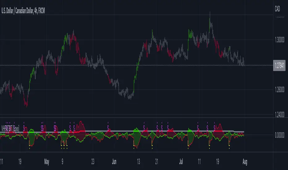
T3 Volatility Quality Index (VQI) w/ DSL & Pips Filtering [Loxx]T3 Volatility Quality Index (VQI) w/ DSL & Pips Filtering is a VQI indicator that uses T3 smoothing and discontinued signal lines to determine breakouts and breakdowns. This also allows filtering by pips.***
What is the Volatility Quality Index ( VQI )?
The idea behind the volatility quality index is to point out the difference between bad and good volatility in order to identify better trade opportunities in the market. This forex indicator works using the True Range algorithm in combination with the open, close, high and low prices.
What are DSL Discontinued Signal Line?
A lot of indicators are using signal lines in order to determine the trend (or some desired state of the indicator) easier. The idea of the signal line is easy : comparing the value to it's smoothed (slightly lagging) state, the idea of current momentum/state is made.
Discontinued signal line is inheriting that simple signal line idea and it is extending it : instead of having one signal line, more lines depending on the current value of the indicator.
"Signal" line is calculated the following way :
When a certain level is crossed into the desired direction, the EMA of that value is calculated for the desired signal line
When that level is crossed into the opposite direction, the previous "signal" line value is simply "inherited" and it becomes a kind of a level
This way it becomes a combination of signal lines and levels that are trying to combine both the good from both methods.
In simple terms, DSL uses the concept of a signal line and betters it by inheriting the previous signal line's value & makes it a level.
What is the T3 moving average?
Better Moving Averages Tim Tillson
November 1, 1998
Tim Tillson is a software project manager at Hewlett-Packard, with degrees in Mathematics and Computer Science. He has privately traded options and equities for 15 years.
Introduction
"Digital filtering includes the process of smoothing, predicting, differentiating, integrating, separation of signals, and removal of noise from a signal. Thus many people who do such things are actually using digital filters without realizing that they are; being unacquainted with the theory, they neither understand what they have done nor the possibilities of what they might have done."
This quote from R. W. Hamming applies to the vast majority of indicators in technical analysis . Moving averages, be they simple, weighted, or exponential, are lowpass filters; low frequency components in the signal pass through with little attenuation, while high frequencies are severely reduced.
"Oscillator" type indicators (such as MACD , Momentum, Relative Strength Index ) are another type of digital filter called a differentiator.
Tushar Chande has observed that many popular oscillators are highly correlated, which is sensible because they are trying to measure the rate of change of the underlying time series, i.e., are trying to be the first and second derivatives we all learned about in Calculus.
We use moving averages (lowpass filters) in technical analysis to remove the random noise from a time series, to discern the underlying trend or to determine prices at which we will take action. A perfect moving average would have two attributes:
It would be smooth, not sensitive to random noise in the underlying time series. Another way of saying this is that its derivative would not spuriously alternate between positive and negative values.
It would not lag behind the time series it is computed from. Lag, of course, produces late buy or sell signals that kill profits.
The only way one can compute a perfect moving average is to have knowledge of the future, and if we had that, we would buy one lottery ticket a week rather than trade!
Having said this, we can still improve on the conventional simple, weighted, or exponential moving averages. Here's how:
Two Interesting Moving Averages
We will examine two benchmark moving averages based on Linear Regression analysis.
In both cases, a Linear Regression line of length n is fitted to price data.
I call the first moving average ILRS, which stands for Integral of Linear Regression Slope. One simply integrates the slope of a linear regression line as it is successively fitted in a moving window of length n across the data, with the constant of integration being a simple moving average of the first n points. Put another way, the derivative of ILRS is the linear regression slope. Note that ILRS is not the same as a SMA ( simple moving average ) of length n, which is actually the midpoint of the linear regression line as it moves across the data.
We can measure the lag of moving averages with respect to a linear trend by computing how they behave when the input is a line with unit slope. Both SMA (n) and ILRS(n) have lag of n/2, but ILRS is much smoother than SMA .
Our second benchmark moving average is well known, called EPMA or End Point Moving Average. It is the endpoint of the linear regression line of length n as it is fitted across the data. EPMA hugs the data more closely than a simple or exponential moving average of the same length. The price we pay for this is that it is much noisier (less smooth) than ILRS, and it also has the annoying property that it overshoots the data when linear trends are present.
However, EPMA has a lag of 0 with respect to linear input! This makes sense because a linear regression line will fit linear input perfectly, and the endpoint of the LR line will be on the input line.
These two moving averages frame the tradeoffs that we are facing. On one extreme we have ILRS, which is very smooth and has considerable phase lag. EPMA has 0 phase lag, but is too noisy and overshoots. We would like to construct a better moving average which is as smooth as ILRS, but runs closer to where EPMA lies, without the overshoot.
A easy way to attempt this is to split the difference, i.e. use (ILRS(n)+EPMA(n))/2. This will give us a moving average (call it IE /2) which runs in between the two, has phase lag of n/4 but still inherits considerable noise from EPMA. IE /2 is inspirational, however. Can we build something that is comparable, but smoother? Figure 1 shows ILRS, EPMA, and IE /2.
Filter Techniques
Any thoughtful student of filter theory (or resolute experimenter) will have noticed that you can improve the smoothness of a filter by running it through itself multiple times, at the cost of increasing phase lag.
There is a complementary technique (called twicing by J.W. Tukey) which can be used to improve phase lag. If L stands for the operation of running data through a low pass filter, then twicing can be described by:
L' = L(time series) + L(time series - L(time series))
That is, we add a moving average of the difference between the input and the moving average to the moving average. This is algebraically equivalent to:
2L-L(L)
This is the Double Exponential Moving Average or DEMA , popularized by Patrick Mulloy in TASAC (January/February 1994).
In our taxonomy, DEMA has some phase lag (although it exponentially approaches 0) and is somewhat noisy, comparable to IE /2 indicator.
We will use these two techniques to construct our better moving average, after we explore the first one a little more closely.
Fixing Overshoot
An n-day EMA has smoothing constant alpha=2/(n+1) and a lag of (n-1)/2.
Thus EMA (3) has lag 1, and EMA (11) has lag 5. Figure 2 shows that, if I am willing to incur 5 days of lag, I get a smoother moving average if I run EMA (3) through itself 5 times than if I just take EMA (11) once.
This suggests that if EPMA and DEMA have 0 or low lag, why not run fast versions (eg DEMA (3)) through themselves many times to achieve a smooth result? The problem is that multiple runs though these filters increase their tendency to overshoot the data, giving an unusable result. This is because the amplitude response of DEMA and EPMA is greater than 1 at certain frequencies, giving a gain of much greater than 1 at these frequencies when run though themselves multiple times. Figure 3 shows DEMA (7) and EPMA(7) run through themselves 3 times. DEMA^3 has serious overshoot, and EPMA^3 is terrible.
The solution to the overshoot problem is to recall what we are doing with twicing:
DEMA (n) = EMA (n) + EMA (time series - EMA (n))
The second term is adding, in effect, a smooth version of the derivative to the EMA to achieve DEMA . The derivative term determines how hot the moving average's response to linear trends will be. We need to simply turn down the volume to achieve our basic building block:
EMA (n) + EMA (time series - EMA (n))*.7;
This is algebraically the same as:
EMA (n)*1.7-EMA( EMA (n))*.7;
I have chosen .7 as my volume factor, but the general formula (which I call "Generalized Dema") is:
GD (n,v) = EMA (n)*(1+v)-EMA( EMA (n))*v,
Where v ranges between 0 and 1. When v=0, GD is just an EMA , and when v=1, GD is DEMA . In between, GD is a cooler DEMA . By using a value for v less than 1 (I like .7), we cure the multiple DEMA overshoot problem, at the cost of accepting some additional phase delay. Now we can run GD through itself multiple times to define a new, smoother moving average T3 that does not overshoot the data:
T3(n) = GD ( GD ( GD (n)))
In filter theory parlance, T3 is a six-pole non-linear Kalman filter. Kalman filters are ones which use the error (in this case (time series - EMA (n)) to correct themselves. In Technical Analysis , these are called Adaptive Moving Averages; they track the time series more aggressively when it is making large moves.
Included
Signals
Alerts
Related indicators
Zero-line Volatility Quality Index (VQI)
Volatility Quality Index w/ Pips Filtering
Variety Moving Average Waddah Attar Explosion (WAE)
***This indicator is tuned to Forex. If you want to make it useful for other tickers, you must change the pip filtering value to match the asset. This means that for BTC, for example, you likely need to use a value of 10,000 or more for pips filter.
In den Scripts nach "Exponential" suchen

VHF-Adaptive T3 iTrend [Loxx]VHF-Adaptive T3 iTrend is an iTrend indicator with T3 smoothing and Vertical Horizontal Filter Adaptive period input. iTrend is used to determine where the trend starts and ends. You'll notice that the noise filter on this one is extreme. Adjust the period inputs accordingly to suit your take and your backtest requirements. This is also useful for scalping lower timeframes. Enjoy!
What is VHF Adaptive Period?
Vertical Horizontal Filter (VHF) was created by Adam White to identify trending and ranging markets. VHF measures the level of trend activity, similar to ADX DI. Vertical Horizontal Filter does not, itself, generate trading signals, but determines whether signals are taken from trend or momentum indicators. Using this trend information, one is then able to derive an average cycle length.
What is the T3 moving average?
Better Moving Averages Tim Tillson
November 1, 1998
Tim Tillson is a software project manager at Hewlett-Packard, with degrees in Mathematics and Computer Science. He has privately traded options and equities for 15 years.
Introduction
"Digital filtering includes the process of smoothing, predicting, differentiating, integrating, separation of signals, and removal of noise from a signal. Thus many people who do such things are actually using digital filters without realizing that they are; being unacquainted with the theory, they neither understand what they have done nor the possibilities of what they might have done."
This quote from R. W. Hamming applies to the vast majority of indicators in technical analysis . Moving averages, be they simple, weighted, or exponential, are lowpass filters; low frequency components in the signal pass through with little attenuation, while high frequencies are severely reduced.
"Oscillator" type indicators (such as MACD , Momentum, Relative Strength Index ) are another type of digital filter called a differentiator.
Tushar Chande has observed that many popular oscillators are highly correlated, which is sensible because they are trying to measure the rate of change of the underlying time series, i.e., are trying to be the first and second derivatives we all learned about in Calculus.
We use moving averages (lowpass filters) in technical analysis to remove the random noise from a time series, to discern the underlying trend or to determine prices at which we will take action. A perfect moving average would have two attributes:
It would be smooth, not sensitive to random noise in the underlying time series. Another way of saying this is that its derivative would not spuriously alternate between positive and negative values.
It would not lag behind the time series it is computed from. Lag, of course, produces late buy or sell signals that kill profits.
The only way one can compute a perfect moving average is to have knowledge of the future, and if we had that, we would buy one lottery ticket a week rather than trade!
Having said this, we can still improve on the conventional simple, weighted, or exponential moving averages. Here's how:
Two Interesting Moving Averages
We will examine two benchmark moving averages based on Linear Regression analysis.
In both cases, a Linear Regression line of length n is fitted to price data.
I call the first moving average ILRS, which stands for Integral of Linear Regression Slope. One simply integrates the slope of a linear regression line as it is successively fitted in a moving window of length n across the data, with the constant of integration being a simple moving average of the first n points. Put another way, the derivative of ILRS is the linear regression slope. Note that ILRS is not the same as a SMA ( simple moving average ) of length n, which is actually the midpoint of the linear regression line as it moves across the data.
We can measure the lag of moving averages with respect to a linear trend by computing how they behave when the input is a line with unit slope. Both SMA (n) and ILRS(n) have lag of n/2, but ILRS is much smoother than SMA .
Our second benchmark moving average is well known, called EPMA or End Point Moving Average. It is the endpoint of the linear regression line of length n as it is fitted across the data. EPMA hugs the data more closely than a simple or exponential moving average of the same length. The price we pay for this is that it is much noisier (less smooth) than ILRS, and it also has the annoying property that it overshoots the data when linear trends are present.
However, EPMA has a lag of 0 with respect to linear input! This makes sense because a linear regression line will fit linear input perfectly, and the endpoint of the LR line will be on the input line.
These two moving averages frame the tradeoffs that we are facing. On one extreme we have ILRS, which is very smooth and has considerable phase lag. EPMA has 0 phase lag, but is too noisy and overshoots. We would like to construct a better moving average which is as smooth as ILRS, but runs closer to where EPMA lies, without the overshoot.
A easy way to attempt this is to split the difference, i.e. use (ILRS(n)+EPMA(n))/2. This will give us a moving average (call it IE /2) which runs in between the two, has phase lag of n/4 but still inherits considerable noise from EPMA. IE /2 is inspirational, however. Can we build something that is comparable, but smoother? Figure 1 shows ILRS, EPMA, and IE /2.
Filter Techniques
Any thoughtful student of filter theory (or resolute experimenter) will have noticed that you can improve the smoothness of a filter by running it through itself multiple times, at the cost of increasing phase lag.
There is a complementary technique (called twicing by J.W. Tukey) which can be used to improve phase lag. If L stands for the operation of running data through a low pass filter, then twicing can be described by:
L' = L(time series) + L(time series - L(time series))
That is, we add a moving average of the difference between the input and the moving average to the moving average. This is algebraically equivalent to:
2L-L(L)
This is the Double Exponential Moving Average or DEMA , popularized by Patrick Mulloy in TASAC (January/February 1994).
In our taxonomy, DEMA has some phase lag (although it exponentially approaches 0) and is somewhat noisy, comparable to IE /2 indicator.
We will use these two techniques to construct our better moving average, after we explore the first one a little more closely.
Fixing Overshoot
An n-day EMA has smoothing constant alpha=2/(n+1) and a lag of (n-1)/2.
Thus EMA (3) has lag 1, and EMA (11) has lag 5. Figure 2 shows that, if I am willing to incur 5 days of lag, I get a smoother moving average if I run EMA (3) through itself 5 times than if I just take EMA (11) once.
This suggests that if EPMA and DEMA have 0 or low lag, why not run fast versions (eg DEMA (3)) through themselves many times to achieve a smooth result? The problem is that multiple runs though these filters increase their tendency to overshoot the data, giving an unusable result. This is because the amplitude response of DEMA and EPMA is greater than 1 at certain frequencies, giving a gain of much greater than 1 at these frequencies when run though themselves multiple times. Figure 3 shows DEMA (7) and EPMA(7) run through themselves 3 times. DEMA^3 has serious overshoot, and EPMA^3 is terrible.
The solution to the overshoot problem is to recall what we are doing with twicing:
DEMA (n) = EMA (n) + EMA (time series - EMA (n))
The second term is adding, in effect, a smooth version of the derivative to the EMA to achieve DEMA . The derivative term determines how hot the moving average's response to linear trends will be. We need to simply turn down the volume to achieve our basic building block:
EMA (n) + EMA (time series - EMA (n))*.7;
This is algebraically the same as:
EMA (n)*1.7-EMA( EMA (n))*.7;
I have chosen .7 as my volume factor, but the general formula (which I call "Generalized Dema") is:
GD (n,v) = EMA (n)*(1+v)-EMA( EMA (n))*v,
Where v ranges between 0 and 1. When v=0, GD is just an EMA , and when v=1, GD is DEMA . In between, GD is a cooler DEMA . By using a value for v less than 1 (I like .7), we cure the multiple DEMA overshoot problem, at the cost of accepting some additional phase delay. Now we can run GD through itself multiple times to define a new, smoother moving average T3 that does not overshoot the data:
T3(n) = GD ( GD ( GD (n)))
In filter theory parlance, T3 is a six-pole non-linear Kalman filter. Kalman filters are ones which use the error (in this case (time series - EMA (n)) to correct themselves. In Technical Analysis , these are called Adaptive Moving Averages; they track the time series more aggressively when it is making large moves.
Included
Bar coloring
Alerts
Signals
Loxx's Expanded Source Types
CFB-Adaptive CCI w/ T3 Smoothing [Loxx]CFB-Adaptive CCI w/ T3 Smoothing is a CCI indicator with adaptive period inputs and T3 smoothing. Jurik's Composite Fractal Behavior is used to created dynamic period input.
What is Composite Fractal Behavior ( CFB )?
All around you mechanisms adjust themselves to their environment. From simple thermostats that react to air temperature to computer chips in modern cars that respond to changes in engine temperature, r.p.m.'s, torque, and throttle position. It was only a matter of time before fast desktop computers applied the mathematics of self-adjustment to systems that trade the financial markets.
Unlike basic systems with fixed formulas, an adaptive system adjusts its own equations. For example, start with a basic channel breakout system that uses the highest closing price of the last N bars as a threshold for detecting breakouts on the up side. An adaptive and improved version of this system would adjust N according to market conditions, such as momentum, price volatility or acceleration.
Since many systems are based directly or indirectly on cycles, another useful measure of market condition is the periodic length of a price chart's dominant cycle, (DC), that cycle with the greatest influence on price action.
The utility of this new DC measure was noted by author Murray Ruggiero in the January '96 issue of Futures Magazine. In it. Mr. Ruggiero used it to adaptive adjust the value of N in a channel breakout system. He then simulated trading 15 years of D-Mark futures in order to compare its performance to a similar system that had a fixed optimal value of N. The adaptive version produced 20% more profit!
This DC index utilized the popular MESA algorithm (a formulation by John Ehlers adapted from Burg's maximum entropy algorithm, MEM). Unfortunately, the DC approach is problematic when the market has no real dominant cycle momentum, because the mathematics will produce a value whether or not one actually exists! Therefore, we developed a proprietary indicator that does not presuppose the presence of market cycles. It's called CFB (Composite Fractal Behavior) and it works well whether or not the market is cyclic.
CFB examines price action for a particular fractal pattern, categorizes them by size, and then outputs a composite fractal size index. This index is smooth, timely and accurate
Essentially, CFB reveals the length of the market's trending action time frame. Long trending activity produces a large CFB index and short choppy action produces a small index value. Investors have found many applications for CFB which involve scaling other existing technical indicators adaptively, on a bar-to-bar basis.
What is Jurik Volty used in the Juirk Filter?
One of the lesser known qualities of Juirk smoothing is that the Jurik smoothing process is adaptive. "Jurik Volty" (a sort of market volatility ) is what makes Jurik smoothing adaptive. The Jurik Volty calculation can be used as both a standalone indicator and to smooth other indicators that you wish to make adaptive.
What is the Jurik Moving Average?
Have you noticed how moving averages add some lag (delay) to your signals? ... especially when price gaps up or down in a big move, and you are waiting for your moving average to catch up? Wait no more! JMA eliminates this problem forever and gives you the best of both worlds: low lag and smooth lines.
Ideally, you would like a filtered signal to be both smooth and lag-free. Lag causes delays in your trades, and increasing lag in your indicators typically result in lower profits. In other words, late comers get what's left on the table after the feast has already begun.
What is the T3 moving average?
Better Moving Averages Tim Tillson
November 1, 1998
Tim Tillson is a software project manager at Hewlett-Packard, with degrees in Mathematics and Computer Science. He has privately traded options and equities for 15 years.
Introduction
"Digital filtering includes the process of smoothing, predicting, differentiating, integrating, separation of signals, and removal of noise from a signal. Thus many people who do such things are actually using digital filters without realizing that they are; being unacquainted with the theory, they neither understand what they have done nor the possibilities of what they might have done."
This quote from R. W. Hamming applies to the vast majority of indicators in technical analysis . Moving averages, be they simple, weighted, or exponential, are lowpass filters; low frequency components in the signal pass through with little attenuation, while high frequencies are severely reduced.
"Oscillator" type indicators (such as MACD , Momentum, Relative Strength Index ) are another type of digital filter called a differentiator.
Tushar Chande has observed that many popular oscillators are highly correlated, which is sensible because they are trying to measure the rate of change of the underlying time series, i.e., are trying to be the first and second derivatives we all learned about in Calculus.
We use moving averages (lowpass filters) in technical analysis to remove the random noise from a time series, to discern the underlying trend or to determine prices at which we will take action. A perfect moving average would have two attributes:
It would be smooth, not sensitive to random noise in the underlying time series. Another way of saying this is that its derivative would not spuriously alternate between positive and negative values.
It would not lag behind the time series it is computed from. Lag, of course, produces late buy or sell signals that kill profits.
The only way one can compute a perfect moving average is to have knowledge of the future, and if we had that, we would buy one lottery ticket a week rather than trade!
Having said this, we can still improve on the conventional simple, weighted, or exponential moving averages. Here's how:
Two Interesting Moving Averages
We will examine two benchmark moving averages based on Linear Regression analysis.
In both cases, a Linear Regression line of length n is fitted to price data.
I call the first moving average ILRS, which stands for Integral of Linear Regression Slope. One simply integrates the slope of a linear regression line as it is successively fitted in a moving window of length n across the data, with the constant of integration being a simple moving average of the first n points. Put another way, the derivative of ILRS is the linear regression slope. Note that ILRS is not the same as a SMA ( simple moving average ) of length n, which is actually the midpoint of the linear regression line as it moves across the data.
We can measure the lag of moving averages with respect to a linear trend by computing how they behave when the input is a line with unit slope. Both SMA (n) and ILRS(n) have lag of n/2, but ILRS is much smoother than SMA .
Our second benchmark moving average is well known, called EPMA or End Point Moving Average. It is the endpoint of the linear regression line of length n as it is fitted across the data. EPMA hugs the data more closely than a simple or exponential moving average of the same length. The price we pay for this is that it is much noisier (less smooth) than ILRS, and it also has the annoying property that it overshoots the data when linear trends are present.
However, EPMA has a lag of 0 with respect to linear input! This makes sense because a linear regression line will fit linear input perfectly, and the endpoint of the LR line will be on the input line.
These two moving averages frame the tradeoffs that we are facing. On one extreme we have ILRS, which is very smooth and has considerable phase lag. EPMA has 0 phase lag, but is too noisy and overshoots. We would like to construct a better moving average which is as smooth as ILRS, but runs closer to where EPMA lies, without the overshoot.
A easy way to attempt this is to split the difference, i.e. use (ILRS(n)+EPMA(n))/2. This will give us a moving average (call it IE /2) which runs in between the two, has phase lag of n/4 but still inherits considerable noise from EPMA. IE /2 is inspirational, however. Can we build something that is comparable, but smoother? Figure 1 shows ILRS, EPMA, and IE /2.
Filter Techniques
Any thoughtful student of filter theory (or resolute experimenter) will have noticed that you can improve the smoothness of a filter by running it through itself multiple times, at the cost of increasing phase lag.
There is a complementary technique (called twicing by J.W. Tukey) which can be used to improve phase lag. If L stands for the operation of running data through a low pass filter, then twicing can be described by:
L' = L(time series) + L(time series - L(time series))
That is, we add a moving average of the difference between the input and the moving average to the moving average. This is algebraically equivalent to:
2L-L(L)
This is the Double Exponential Moving Average or DEMA , popularized by Patrick Mulloy in TASAC (January/February 1994).
In our taxonomy, DEMA has some phase lag (although it exponentially approaches 0) and is somewhat noisy, comparable to IE /2 indicator.
We will use these two techniques to construct our better moving average, after we explore the first one a little more closely.
Fixing Overshoot
An n-day EMA has smoothing constant alpha=2/(n+1) and a lag of (n-1)/2.
Thus EMA (3) has lag 1, and EMA (11) has lag 5. Figure 2 shows that, if I am willing to incur 5 days of lag, I get a smoother moving average if I run EMA (3) through itself 5 times than if I just take EMA (11) once.
This suggests that if EPMA and DEMA have 0 or low lag, why not run fast versions (eg DEMA (3)) through themselves many times to achieve a smooth result? The problem is that multiple runs though these filters increase their tendency to overshoot the data, giving an unusable result. This is because the amplitude response of DEMA and EPMA is greater than 1 at certain frequencies, giving a gain of much greater than 1 at these frequencies when run though themselves multiple times. Figure 3 shows DEMA (7) and EPMA(7) run through themselves 3 times. DEMA^3 has serious overshoot, and EPMA^3 is terrible.
The solution to the overshoot problem is to recall what we are doing with twicing:
DEMA (n) = EMA (n) + EMA (time series - EMA (n))
The second term is adding, in effect, a smooth version of the derivative to the EMA to achieve DEMA . The derivative term determines how hot the moving average's response to linear trends will be. We need to simply turn down the volume to achieve our basic building block:
EMA (n) + EMA (time series - EMA (n))*.7;
This is algebraically the same as:
EMA (n)*1.7-EMA( EMA (n))*.7;
I have chosen .7 as my volume factor, but the general formula (which I call "Generalized Dema") is:
GD (n,v) = EMA (n)*(1+v)-EMA( EMA (n))*v,
Where v ranges between 0 and 1. When v=0, GD is just an EMA , and when v=1, GD is DEMA . In between, GD is a cooler DEMA . By using a value for v less than 1 (I like .7), we cure the multiple DEMA overshoot problem, at the cost of accepting some additional phase delay. Now we can run GD through itself multiple times to define a new, smoother moving average T3 that does not overshoot the data:
T3(n) = GD ( GD ( GD (n)))
In filter theory parlance, T3 is a six-pole non-linear Kalman filter. Kalman filters are ones which use the error (in this case (time series - EMA (n)) to correct themselves. In Technical Analysis , these are called Adaptive Moving Averages; they track the time series more aggressively when it is making large moves.
Included:
Bar coloring
Signals
Alerts

STD-Adaptive T3 Channel w/ Ehlers Swiss Army Knife Mod. [Loxx]STD-Adaptive T3 Channel w/ Ehlers Swiss Army Knife Mod. is an adaptive T3 indicator using standard deviation adaptivity and Ehlers Swiss Army Knife indicator to adjust the alpha value of the T3 calculation. This helps identify trends and reduce noise. In addition. I've included a Keltner Channel to show reversal/exhaustion zones.
What is the Swiss Army Knife Indicator?
John Ehlers explains the calculation here: www.mesasoftware.com
What is the T3 moving average?
Better Moving Averages Tim Tillson
November 1, 1998
Tim Tillson is a software project manager at Hewlett-Packard, with degrees in Mathematics and Computer Science. He has privately traded options and equities for 15 years.
Introduction
"Digital filtering includes the process of smoothing, predicting, differentiating, integrating, separation of signals, and removal of noise from a signal. Thus many people who do such things are actually using digital filters without realizing that they are; being unacquainted with the theory, they neither understand what they have done nor the possibilities of what they might have done."
This quote from R. W. Hamming applies to the vast majority of indicators in technical analysis . Moving averages, be they simple, weighted, or exponential, are lowpass filters; low frequency components in the signal pass through with little attenuation, while high frequencies are severely reduced.
"Oscillator" type indicators (such as MACD , Momentum, Relative Strength Index ) are another type of digital filter called a differentiator.
Tushar Chande has observed that many popular oscillators are highly correlated, which is sensible because they are trying to measure the rate of change of the underlying time series, i.e., are trying to be the first and second derivatives we all learned about in Calculus.
We use moving averages (lowpass filters) in technical analysis to remove the random noise from a time series, to discern the underlying trend or to determine prices at which we will take action. A perfect moving average would have two attributes:
It would be smooth, not sensitive to random noise in the underlying time series. Another way of saying this is that its derivative would not spuriously alternate between positive and negative values.
It would not lag behind the time series it is computed from. Lag, of course, produces late buy or sell signals that kill profits.
The only way one can compute a perfect moving average is to have knowledge of the future, and if we had that, we would buy one lottery ticket a week rather than trade!
Having said this, we can still improve on the conventional simple, weighted, or exponential moving averages. Here's how:
Two Interesting Moving Averages
We will examine two benchmark moving averages based on Linear Regression analysis.
In both cases, a Linear Regression line of length n is fitted to price data.
I call the first moving average ILRS, which stands for Integral of Linear Regression Slope. One simply integrates the slope of a linear regression line as it is successively fitted in a moving window of length n across the data, with the constant of integration being a simple moving average of the first n points. Put another way, the derivative of ILRS is the linear regression slope. Note that ILRS is not the same as a SMA ( simple moving average ) of length n, which is actually the midpoint of the linear regression line as it moves across the data.
We can measure the lag of moving averages with respect to a linear trend by computing how they behave when the input is a line with unit slope. Both SMA (n) and ILRS(n) have lag of n/2, but ILRS is much smoother than SMA .
Our second benchmark moving average is well known, called EPMA or End Point Moving Average. It is the endpoint of the linear regression line of length n as it is fitted across the data. EPMA hugs the data more closely than a simple or exponential moving average of the same length. The price we pay for this is that it is much noisier (less smooth) than ILRS, and it also has the annoying property that it overshoots the data when linear trends are present.
However, EPMA has a lag of 0 with respect to linear input! This makes sense because a linear regression line will fit linear input perfectly, and the endpoint of the LR line will be on the input line.
These two moving averages frame the tradeoffs that we are facing. On one extreme we have ILRS, which is very smooth and has considerable phase lag. EPMA has 0 phase lag, but is too noisy and overshoots. We would like to construct a better moving average which is as smooth as ILRS, but runs closer to where EPMA lies, without the overshoot.
A easy way to attempt this is to split the difference, i.e. use (ILRS(n)+EPMA(n))/2. This will give us a moving average (call it IE /2) which runs in between the two, has phase lag of n/4 but still inherits considerable noise from EPMA. IE /2 is inspirational, however. Can we build something that is comparable, but smoother? Figure 1 shows ILRS, EPMA, and IE /2.
Filter Techniques
Any thoughtful student of filter theory (or resolute experimenter) will have noticed that you can improve the smoothness of a filter by running it through itself multiple times, at the cost of increasing phase lag.
There is a complementary technique (called twicing by J.W. Tukey) which can be used to improve phase lag. If L stands for the operation of running data through a low pass filter, then twicing can be described by:
L' = L(time series) + L(time series - L(time series))
That is, we add a moving average of the difference between the input and the moving average to the moving average. This is algebraically equivalent to:
2L-L(L)
This is the Double Exponential Moving Average or DEMA , popularized by Patrick Mulloy in TASAC (January/February 1994).
In our taxonomy, DEMA has some phase lag (although it exponentially approaches 0) and is somewhat noisy, comparable to IE /2 indicator.
We will use these two techniques to construct our better moving average, after we explore the first one a little more closely.
Fixing Overshoot
An n-day EMA has smoothing constant alpha=2/(n+1) and a lag of (n-1)/2.
Thus EMA (3) has lag 1, and EMA (11) has lag 5. Figure 2 shows that, if I am willing to incur 5 days of lag, I get a smoother moving average if I run EMA (3) through itself 5 times than if I just take EMA (11) once.
This suggests that if EPMA and DEMA have 0 or low lag, why not run fast versions (eg DEMA (3)) through themselves many times to achieve a smooth result? The problem is that multiple runs though these filters increase their tendency to overshoot the data, giving an unusable result. This is because the amplitude response of DEMA and EPMA is greater than 1 at certain frequencies, giving a gain of much greater than 1 at these frequencies when run though themselves multiple times. Figure 3 shows DEMA (7) and EPMA(7) run through themselves 3 times. DEMA^3 has serious overshoot, and EPMA^3 is terrible.
The solution to the overshoot problem is to recall what we are doing with twicing:
DEMA (n) = EMA (n) + EMA (time series - EMA (n))
The second term is adding, in effect, a smooth version of the derivative to the EMA to achieve DEMA . The derivative term determines how hot the moving average's response to linear trends will be. We need to simply turn down the volume to achieve our basic building block:
EMA (n) + EMA (time series - EMA (n))*.7;
This is algebraically the same as:
EMA (n)*1.7-EMA( EMA (n))*.7;
I have chosen .7 as my volume factor, but the general formula (which I call "Generalized Dema") is:
GD (n,v) = EMA (n)*(1+v)-EMA( EMA (n))*v,
Where v ranges between 0 and 1. When v=0, GD is just an EMA , and when v=1, GD is DEMA . In between, GD is a cooler DEMA . By using a value for v less than 1 (I like .7), we cure the multiple DEMA overshoot problem, at the cost of accepting some additional phase delay. Now we can run GD through itself multiple times to define a new, smoother moving average T3 that does not overshoot the data:
T3(n) = GD ( GD ( GD (n)))
In filter theory parlance, T3 is a six-pole non-linear Kalman filter. Kalman filters are ones which use the error (in this case (time series - EMA (n)) to correct themselves. In Technical Analysis , these are called Adaptive Moving Averages; they track the time series more aggressively when it is making large moves.
Included:
Bar coloring
Signals
Alerts
Loxx's Expanded Source Types
T3 Velocity [Loxx]T3 Velocity is a simple velocity indicator using T3 moving average that uses gradient colors to better identify trends.
What is the T3 moving average?
Better Moving Averages Tim Tillson
November 1, 1998
Tim Tillson is a software project manager at Hewlett-Packard, with degrees in Mathematics and Computer Science. He has privately traded options and equities for 15 years.
Introduction
"Digital filtering includes the process of smoothing, predicting, differentiating, integrating, separation of signals, and removal of noise from a signal. Thus many people who do such things are actually using digital filters without realizing that they are; being unacquainted with the theory, they neither understand what they have done nor the possibilities of what they might have done."
This quote from R. W. Hamming applies to the vast majority of indicators in technical analysis . Moving averages, be they simple, weighted, or exponential, are lowpass filters; low frequency components in the signal pass through with little attenuation, while high frequencies are severely reduced.
"Oscillator" type indicators (such as MACD , Momentum, Relative Strength Index ) are another type of digital filter called a differentiator.
Tushar Chande has observed that many popular oscillators are highly correlated, which is sensible because they are trying to measure the rate of change of the underlying time series, i.e., are trying to be the first and second derivatives we all learned about in Calculus.
We use moving averages (lowpass filters) in technical analysis to remove the random noise from a time series, to discern the underlying trend or to determine prices at which we will take action. A perfect moving average would have two attributes:
It would be smooth, not sensitive to random noise in the underlying time series. Another way of saying this is that its derivative would not spuriously alternate between positive and negative values.
It would not lag behind the time series it is computed from. Lag, of course, produces late buy or sell signals that kill profits.
The only way one can compute a perfect moving average is to have knowledge of the future, and if we had that, we would buy one lottery ticket a week rather than trade!
Having said this, we can still improve on the conventional simple, weighted, or exponential moving averages. Here's how:
Two Interesting Moving Averages
We will examine two benchmark moving averages based on Linear Regression analysis.
In both cases, a Linear Regression line of length n is fitted to price data.
I call the first moving average ILRS, which stands for Integral of Linear Regression Slope. One simply integrates the slope of a linear regression line as it is successively fitted in a moving window of length n across the data, with the constant of integration being a simple moving average of the first n points. Put another way, the derivative of ILRS is the linear regression slope. Note that ILRS is not the same as a SMA ( simple moving average ) of length n, which is actually the midpoint of the linear regression line as it moves across the data.
We can measure the lag of moving averages with respect to a linear trend by computing how they behave when the input is a line with unit slope. Both SMA (n) and ILRS(n) have lag of n/2, but ILRS is much smoother than SMA .
Our second benchmark moving average is well known, called EPMA or End Point Moving Average. It is the endpoint of the linear regression line of length n as it is fitted across the data. EPMA hugs the data more closely than a simple or exponential moving average of the same length. The price we pay for this is that it is much noisier (less smooth) than ILRS, and it also has the annoying property that it overshoots the data when linear trends are present.
However, EPMA has a lag of 0 with respect to linear input! This makes sense because a linear regression line will fit linear input perfectly, and the endpoint of the LR line will be on the input line.
These two moving averages frame the tradeoffs that we are facing. On one extreme we have ILRS, which is very smooth and has considerable phase lag. EPMA has 0 phase lag, but is too noisy and overshoots. We would like to construct a better moving average which is as smooth as ILRS, but runs closer to where EPMA lies, without the overshoot.
A easy way to attempt this is to split the difference, i.e. use (ILRS(n)+EPMA(n))/2. This will give us a moving average (call it IE /2) which runs in between the two, has phase lag of n/4 but still inherits considerable noise from EPMA. IE /2 is inspirational, however. Can we build something that is comparable, but smoother? Figure 1 shows ILRS, EPMA, and IE /2.
Filter Techniques
Any thoughtful student of filter theory (or resolute experimenter) will have noticed that you can improve the smoothness of a filter by running it through itself multiple times, at the cost of increasing phase lag.
There is a complementary technique (called twicing by J.W. Tukey) which can be used to improve phase lag. If L stands for the operation of running data through a low pass filter, then twicing can be described by:
L' = L(time series) + L(time series - L(time series))
That is, we add a moving average of the difference between the input and the moving average to the moving average. This is algebraically equivalent to:
2L-L(L)
This is the Double Exponential Moving Average or DEMA , popularized by Patrick Mulloy in TASAC (January/February 1994).
In our taxonomy, DEMA has some phase lag (although it exponentially approaches 0) and is somewhat noisy, comparable to IE /2 indicator.
We will use these two techniques to construct our better moving average, after we explore the first one a little more closely.
Fixing Overshoot
An n-day EMA has smoothing constant alpha=2/(n+1) and a lag of (n-1)/2.
Thus EMA (3) has lag 1, and EMA (11) has lag 5. Figure 2 shows that, if I am willing to incur 5 days of lag, I get a smoother moving average if I run EMA (3) through itself 5 times than if I just take EMA (11) once.
This suggests that if EPMA and DEMA have 0 or low lag, why not run fast versions (eg DEMA (3)) through themselves many times to achieve a smooth result? The problem is that multiple runs though these filters increase their tendency to overshoot the data, giving an unusable result. This is because the amplitude response of DEMA and EPMA is greater than 1 at certain frequencies, giving a gain of much greater than 1 at these frequencies when run though themselves multiple times. Figure 3 shows DEMA (7) and EPMA(7) run through themselves 3 times. DEMA^3 has serious overshoot, and EPMA^3 is terrible.
The solution to the overshoot problem is to recall what we are doing with twicing:
DEMA (n) = EMA (n) + EMA (time series - EMA (n))
The second term is adding, in effect, a smooth version of the derivative to the EMA to achieve DEMA . The derivative term determines how hot the moving average's response to linear trends will be. We need to simply turn down the volume to achieve our basic building block:
EMA (n) + EMA (time series - EMA (n))*.7;
This is algebraically the same as:
EMA (n)*1.7-EMA( EMA (n))*.7;
I have chosen .7 as my volume factor, but the general formula (which I call "Generalized Dema") is:
GD (n,v) = EMA (n)*(1+v)-EMA( EMA (n))*v,
Where v ranges between 0 and 1. When v=0, GD is just an EMA , and when v=1, GD is DEMA . In between, GD is a cooler DEMA . By using a value for v less than 1 (I like .7), we cure the multiple DEMA overshoot problem, at the cost of accepting some additional phase delay. Now we can run GD through itself multiple times to define a new, smoother moving average T3 that does not overshoot the data:
T3(n) = GD ( GD ( GD (n)))
In filter theory parlance, T3 is a six-pole non-linear Kalman filter. Kalman filters are ones which use the error (in this case (time series - EMA (n)) to correct themselves. In Technical Analysis , these are called Adaptive Moving Averages; they track the time series more aggressively when it is making large moves.
Included:
Bar coloring
Signals
Alerts
Loxx's Expanded Source Types

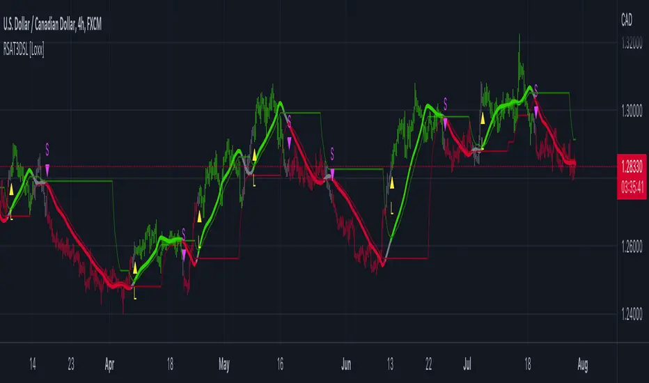
R-squared Adaptive T3 w/ DSL [Loxx]R-squared Adaptive T3 w/ DSL is the following T3 indicator but with Discontinued Signal Lines added to reduce noise and thereby increase signal accuracy. This adaptation makes this indicator lower TF scalp friendly.
What is R-squared Adaptive?
One tool available in forecasting the trendiness of the breakout is the coefficient of determination ( R-squared ), a statistical measurement.
The R-squared indicates linear strength between the security's price (the Y - axis) and time (the X - axis). The R-squared is the percentage of squared error that the linear regression can eliminate if it were used as the predictor instead of the mean value. If the R-squared were 0.99, then the linear regression would eliminate 99% of the error for prediction versus predicting closing prices using a simple moving average .
R-squared is used here to derive a T3 factor used to modify price before passing price through a six-pole non-linear Kalman filter.
What is the T3 moving average?
Better Moving Averages Tim Tillson
November 1, 1998
Tim Tillson is a software project manager at Hewlett-Packard, with degrees in Mathematics and Computer Science. He has privately traded options and equities for 15 years.
Introduction
"Digital filtering includes the process of smoothing, predicting, differentiating, integrating, separation of signals, and removal of noise from a signal. Thus many people who do such things are actually using digital filters without realizing that they are; being unacquainted with the theory, they neither understand what they have done nor the possibilities of what they might have done."
This quote from R. W. Hamming applies to the vast majority of indicators in technical analysis . Moving averages, be they simple, weighted, or exponential, are lowpass filters; low frequency components in the signal pass through with little attenuation, while high frequencies are severely reduced.
"Oscillator" type indicators (such as MACD , Momentum, Relative Strength Index ) are another type of digital filter called a differentiator.
Tushar Chande has observed that many popular oscillators are highly correlated, which is sensible because they are trying to measure the rate of change of the underlying time series, i.e., are trying to be the first and second derivatives we all learned about in Calculus.
We use moving averages (lowpass filters) in technical analysis to remove the random noise from a time series, to discern the underlying trend or to determine prices at which we will take action. A perfect moving average would have two attributes:
It would be smooth, not sensitive to random noise in the underlying time series. Another way of saying this is that its derivative would not spuriously alternate between positive and negative values.
It would not lag behind the time series it is computed from. Lag, of course, produces late buy or sell signals that kill profits.
The only way one can compute a perfect moving average is to have knowledge of the future, and if we had that, we would buy one lottery ticket a week rather than trade!
Having said this, we can still improve on the conventional simple, weighted, or exponential moving averages. Here's how:
Two Interesting Moving Averages
We will examine two benchmark moving averages based on Linear Regression analysis.
In both cases, a Linear Regression line of length n is fitted to price data.
I call the first moving average ILRS, which stands for Integral of Linear Regression Slope. One simply integrates the slope of a linear regression line as it is successively fitted in a moving window of length n across the data, with the constant of integration being a simple moving average of the first n points. Put another way, the derivative of ILRS is the linear regression slope. Note that ILRS is not the same as a SMA ( simple moving average ) of length n, which is actually the midpoint of the linear regression line as it moves across the data.
We can measure the lag of moving averages with respect to a linear trend by computing how they behave when the input is a line with unit slope. Both SMA (n) and ILRS(n) have lag of n/2, but ILRS is much smoother than SMA .
Our second benchmark moving average is well known, called EPMA or End Point Moving Average. It is the endpoint of the linear regression line of length n as it is fitted across the data. EPMA hugs the data more closely than a simple or exponential moving average of the same length. The price we pay for this is that it is much noisier (less smooth) than ILRS, and it also has the annoying property that it overshoots the data when linear trends are present.
However, EPMA has a lag of 0 with respect to linear input! This makes sense because a linear regression line will fit linear input perfectly, and the endpoint of the LR line will be on the input line.
These two moving averages frame the tradeoffs that we are facing. On one extreme we have ILRS, which is very smooth and has considerable phase lag. EPMA has 0 phase lag, but is too noisy and overshoots. We would like to construct a better moving average which is as smooth as ILRS, but runs closer to where EPMA lies, without the overshoot.
A easy way to attempt this is to split the difference, i.e. use (ILRS(n)+EPMA(n))/2. This will give us a moving average (call it IE /2) which runs in between the two, has phase lag of n/4 but still inherits considerable noise from EPMA. IE /2 is inspirational, however. Can we build something that is comparable, but smoother? Figure 1 shows ILRS, EPMA, and IE /2.
Filter Techniques
Any thoughtful student of filter theory (or resolute experimenter) will have noticed that you can improve the smoothness of a filter by running it through itself multiple times, at the cost of increasing phase lag.
There is a complementary technique (called twicing by J.W. Tukey) which can be used to improve phase lag. If L stands for the operation of running data through a low pass filter, then twicing can be described by:
L' = L(time series) + L(time series - L(time series))
That is, we add a moving average of the difference between the input and the moving average to the moving average. This is algebraically equivalent to:
2L-L(L)
This is the Double Exponential Moving Average or DEMA , popularized by Patrick Mulloy in TASAC (January/February 1994).
In our taxonomy, DEMA has some phase lag (although it exponentially approaches 0) and is somewhat noisy, comparable to IE /2 indicator.
We will use these two techniques to construct our better moving average, after we explore the first one a little more closely.
Fixing Overshoot
An n-day EMA has smoothing constant alpha=2/(n+1) and a lag of (n-1)/2.
Thus EMA (3) has lag 1, and EMA (11) has lag 5. Figure 2 shows that, if I am willing to incur 5 days of lag, I get a smoother moving average if I run EMA (3) through itself 5 times than if I just take EMA (11) once.
This suggests that if EPMA and DEMA have 0 or low lag, why not run fast versions (eg DEMA (3)) through themselves many times to achieve a smooth result? The problem is that multiple runs though these filters increase their tendency to overshoot the data, giving an unusable result. This is because the amplitude response of DEMA and EPMA is greater than 1 at certain frequencies, giving a gain of much greater than 1 at these frequencies when run though themselves multiple times. Figure 3 shows DEMA (7) and EPMA(7) run through themselves 3 times. DEMA^3 has serious overshoot, and EPMA^3 is terrible.
The solution to the overshoot problem is to recall what we are doing with twicing:
DEMA (n) = EMA (n) + EMA (time series - EMA (n))
The second term is adding, in effect, a smooth version of the derivative to the EMA to achieve DEMA . The derivative term determines how hot the moving average's response to linear trends will be. We need to simply turn down the volume to achieve our basic building block:
EMA (n) + EMA (time series - EMA (n))*.7;
This is algebraically the same as:
EMA (n)*1.7-EMA( EMA (n))*.7;
I have chosen .7 as my volume factor, but the general formula (which I call "Generalized Dema") is:
GD (n,v) = EMA (n)*(1+v)-EMA( EMA (n))*v,
Where v ranges between 0 and 1. When v=0, GD is just an EMA , and when v=1, GD is DEMA . In between, GD is a cooler DEMA . By using a value for v less than 1 (I like .7), we cure the multiple DEMA overshoot problem, at the cost of accepting some additional phase delay. Now we can run GD through itself multiple times to define a new, smoother moving average T3 that does not overshoot the data:
T3(n) = GD ( GD ( GD (n)))
In filter theory parlance, T3 is a six-pole non-linear Kalman filter. Kalman filters are ones which use the error (in this case (time series - EMA (n)) to correct themselves. In Technical Analysis , these are called Adaptive Moving Averages; they track the time series more aggressively when it is making large moves.
Included:
Bar coloring
Signals
Alerts
EMA and FEMA Signla/DSL smoothing
Loxx's Expanded Source Types
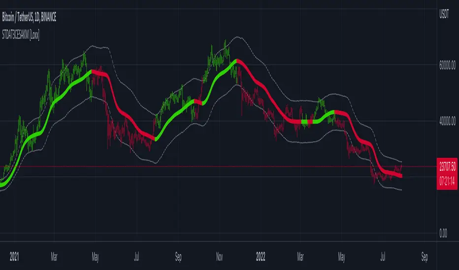
STD-Filterd, R-squared Adaptive T3 w/ Dynamic Zones [Loxx]STD-Filterd, R-squared Adaptive T3 w/ Dynamic Zones is a standard deviation filtered R-squared Adaptive T3 moving average with dynamic zones.
What is the T3 moving average?
Better Moving Averages Tim Tillson
November 1, 1998
Tim Tillson is a software project manager at Hewlett-Packard, with degrees in Mathematics and Computer Science. He has privately traded options and equities for 15 years.
Introduction
"Digital filtering includes the process of smoothing, predicting, differentiating, integrating, separation of signals, and removal of noise from a signal. Thus many people who do such things are actually using digital filters without realizing that they are; being unacquainted with the theory, they neither understand what they have done nor the possibilities of what they might have done."
This quote from R. W. Hamming applies to the vast majority of indicators in technical analysis . Moving averages, be they simple, weighted, or exponential, are lowpass filters; low frequency components in the signal pass through with little attenuation, while high frequencies are severely reduced.
"Oscillator" type indicators (such as MACD , Momentum, Relative Strength Index ) are another type of digital filter called a differentiator.
Tushar Chande has observed that many popular oscillators are highly correlated, which is sensible because they are trying to measure the rate of change of the underlying time series, i.e., are trying to be the first and second derivatives we all learned about in Calculus.
We use moving averages (lowpass filters) in technical analysis to remove the random noise from a time series, to discern the underlying trend or to determine prices at which we will take action. A perfect moving average would have two attributes:
It would be smooth, not sensitive to random noise in the underlying time series. Another way of saying this is that its derivative would not spuriously alternate between positive and negative values.
It would not lag behind the time series it is computed from. Lag, of course, produces late buy or sell signals that kill profits.
The only way one can compute a perfect moving average is to have knowledge of the future, and if we had that, we would buy one lottery ticket a week rather than trade!
Having said this, we can still improve on the conventional simple, weighted, or exponential moving averages. Here's how:
Two Interesting Moving Averages
We will examine two benchmark moving averages based on Linear Regression analysis.
In both cases, a Linear Regression line of length n is fitted to price data.
I call the first moving average ILRS, which stands for Integral of Linear Regression Slope. One simply integrates the slope of a linear regression line as it is successively fitted in a moving window of length n across the data, with the constant of integration being a simple moving average of the first n points. Put another way, the derivative of ILRS is the linear regression slope. Note that ILRS is not the same as a SMA ( simple moving average ) of length n, which is actually the midpoint of the linear regression line as it moves across the data.
We can measure the lag of moving averages with respect to a linear trend by computing how they behave when the input is a line with unit slope. Both SMA (n) and ILRS(n) have lag of n/2, but ILRS is much smoother than SMA .
Our second benchmark moving average is well known, called EPMA or End Point Moving Average. It is the endpoint of the linear regression line of length n as it is fitted across the data. EPMA hugs the data more closely than a simple or exponential moving average of the same length. The price we pay for this is that it is much noisier (less smooth) than ILRS, and it also has the annoying property that it overshoots the data when linear trends are present.
However, EPMA has a lag of 0 with respect to linear input! This makes sense because a linear regression line will fit linear input perfectly, and the endpoint of the LR line will be on the input line.
These two moving averages frame the tradeoffs that we are facing. On one extreme we have ILRS, which is very smooth and has considerable phase lag. EPMA has 0 phase lag, but is too noisy and overshoots. We would like to construct a better moving average which is as smooth as ILRS, but runs closer to where EPMA lies, without the overshoot.
A easy way to attempt this is to split the difference, i.e. use (ILRS(n)+EPMA(n))/2. This will give us a moving average (call it IE /2) which runs in between the two, has phase lag of n/4 but still inherits considerable noise from EPMA. IE /2 is inspirational, however. Can we build something that is comparable, but smoother? Figure 1 shows ILRS, EPMA, and IE /2.
Filter Techniques
Any thoughtful student of filter theory (or resolute experimenter) will have noticed that you can improve the smoothness of a filter by running it through itself multiple times, at the cost of increasing phase lag.
There is a complementary technique (called twicing by J.W. Tukey) which can be used to improve phase lag. If L stands for the operation of running data through a low pass filter, then twicing can be described by:
L' = L(time series) + L(time series - L(time series))
That is, we add a moving average of the difference between the input and the moving average to the moving average. This is algebraically equivalent to:
2L-L(L)
This is the Double Exponential Moving Average or DEMA , popularized by Patrick Mulloy in TASAC (January/February 1994).
In our taxonomy, DEMA has some phase lag (although it exponentially approaches 0) and is somewhat noisy, comparable to IE /2 indicator.
We will use these two techniques to construct our better moving average, after we explore the first one a little more closely.
Fixing Overshoot
An n-day EMA has smoothing constant alpha=2/(n+1) and a lag of (n-1)/2.
Thus EMA (3) has lag 1, and EMA (11) has lag 5. Figure 2 shows that, if I am willing to incur 5 days of lag, I get a smoother moving average if I run EMA (3) through itself 5 times than if I just take EMA (11) once.
This suggests that if EPMA and DEMA have 0 or low lag, why not run fast versions (eg DEMA (3)) through themselves many times to achieve a smooth result? The problem is that multiple runs though these filters increase their tendency to overshoot the data, giving an unusable result. This is because the amplitude response of DEMA and EPMA is greater than 1 at certain frequencies, giving a gain of much greater than 1 at these frequencies when run though themselves multiple times. Figure 3 shows DEMA (7) and EPMA(7) run through themselves 3 times. DEMA^3 has serious overshoot, and EPMA^3 is terrible.
The solution to the overshoot problem is to recall what we are doing with twicing:
DEMA (n) = EMA (n) + EMA (time series - EMA (n))
The second term is adding, in effect, a smooth version of the derivative to the EMA to achieve DEMA . The derivative term determines how hot the moving average's response to linear trends will be. We need to simply turn down the volume to achieve our basic building block:
EMA (n) + EMA (time series - EMA (n))*.7;
This is algebraically the same as:
EMA (n)*1.7-EMA( EMA (n))*.7;
I have chosen .7 as my volume factor, but the general formula (which I call "Generalized Dema") is:
GD (n,v) = EMA (n)*(1+v)-EMA( EMA (n))*v,
Where v ranges between 0 and 1. When v=0, GD is just an EMA , and when v=1, GD is DEMA . In between, GD is a cooler DEMA . By using a value for v less than 1 (I like .7), we cure the multiple DEMA overshoot problem, at the cost of accepting some additional phase delay. Now we can run GD through itself multiple times to define a new, smoother moving average T3 that does not overshoot the data:
T3(n) = GD ( GD ( GD (n)))
In filter theory parlance, T3 is a six-pole non-linear Kalman filter. Kalman filters are ones which use the error (in this case (time series - EMA (n)) to correct themselves. In Technical Analysis , these are called Adaptive Moving Averages; they track the time series more aggressively when it is making large moves.
What is R-squared Adaptive?
One tool available in forecasting the trendiness of the breakout is the coefficient of determination ( R-squared ), a statistical measurement.
The R-squared indicates linear strength between the security's price (the Y - axis) and time (the X - axis). The R-squared is the percentage of squared error that the linear regression can eliminate if it were used as the predictor instead of the mean value. If the R-squared were 0.99, then the linear regression would eliminate 99% of the error for prediction versus predicting closing prices using a simple moving average .
R-squared is used here to derive a T3 factor used to modify price before passing price through a six-pole non-linear Kalman filter.
What are Dynamic Zones?
As explained in "Stocks & Commodities V15:7 (306-310): Dynamic Zones by Leo Zamansky, Ph .D., and David Stendahl"
Most indicators use a fixed zone for buy and sell signals. Here’ s a concept based on zones that are responsive to past levels of the indicator.
One approach to active investing employs the use of oscillators to exploit tradable market trends. This investing style follows a very simple form of logic: Enter the market only when an oscillator has moved far above or below traditional trading lev- els. However, these oscillator- driven systems lack the ability to evolve with the market because they use fixed buy and sell zones. Traders typically use one set of buy and sell zones for a bull market and substantially different zones for a bear market. And therein lies the problem.
Once traders begin introducing their market opinions into trading equations, by changing the zones, they negate the system’s mechanical nature. The objective is to have a system automatically define its own buy and sell zones and thereby profitably trade in any market — bull or bear. Dynamic zones offer a solution to the problem of fixed buy and sell zones for any oscillator-driven system.
An indicator’s extreme levels can be quantified using statistical methods. These extreme levels are calculated for a certain period and serve as the buy and sell zones for a trading system. The repetition of this statistical process for every value of the indicator creates values that become the dynamic zones. The zones are calculated in such a way that the probability of the indicator value rising above, or falling below, the dynamic zones is equal to a given probability input set by the trader.
To better understand dynamic zones, let's first describe them mathematically and then explain their use. The dynamic zones definition:
Find V such that:
For dynamic zone buy: P{X <= V}=P1
For dynamic zone sell: P{X >= V}=P2
where P1 and P2 are the probabilities set by the trader, X is the value of the indicator for the selected period and V represents the value of the dynamic zone.
The probability input P1 and P2 can be adjusted by the trader to encompass as much or as little data as the trader would like. The smaller the probability, the fewer data values above and below the dynamic zones. This translates into a wider range between the buy and sell zones. If a 10% probability is used for P1 and P2, only those data values that make up the top 10% and bottom 10% for an indicator are used in the construction of the zones. Of the values, 80% will fall between the two extreme levels. Because dynamic zone levels are penetrated so infrequently, when this happens, traders know that the market has truly moved into overbought or oversold territory.
Calculating the Dynamic Zones
The algorithm for the dynamic zones is a series of steps. First, decide the value of the lookback period t. Next, decide the value of the probability Pbuy for buy zone and value of the probability Psell for the sell zone.
For i=1, to the last lookback period, build the distribution f(x) of the price during the lookback period i. Then find the value Vi1 such that the probability of the price less than or equal to Vi1 during the lookback period i is equal to Pbuy. Find the value Vi2 such that the probability of the price greater or equal to Vi2 during the lookback period i is equal to Psell. The sequence of Vi1 for all periods gives the buy zone. The sequence of Vi2 for all periods gives the sell zone.
In the algorithm description, we have: Build the distribution f(x) of the price during the lookback period i. The distribution here is empirical namely, how many times a given value of x appeared during the lookback period. The problem is to find such x that the probability of a price being greater or equal to x will be equal to a probability selected by the user. Probability is the area under the distribution curve. The task is to find such value of x that the area under the distribution curve to the right of x will be equal to the probability selected by the user. That x is the dynamic zone.
Included:
Bar coloring
Signals
Alerts
Loxx's Expanded Source Types

Pips-Stepped, R-squared Adaptive T3 [Loxx]Pips-Stepped, R-squared Adaptive T3 is a a T3 moving average with optional adaptivity, trend following, and pip-stepping. This indicator also uses optional flat coloring to determine chops zones. This indicator is R-squared adaptive. This is also an experimental indicator.
What is the T3 moving average?
Better Moving Averages Tim Tillson
November 1, 1998
Tim Tillson is a software project manager at Hewlett-Packard, with degrees in Mathematics and Computer Science. He has privately traded options and equities for 15 years.
Introduction
"Digital filtering includes the process of smoothing, predicting, differentiating, integrating, separation of signals, and removal of noise from a signal. Thus many people who do such things are actually using digital filters without realizing that they are; being unacquainted with the theory, they neither understand what they have done nor the possibilities of what they might have done."
This quote from R. W. Hamming applies to the vast majority of indicators in technical analysis . Moving averages, be they simple, weighted, or exponential, are lowpass filters; low frequency components in the signal pass through with little attenuation, while high frequencies are severely reduced.
"Oscillator" type indicators (such as MACD , Momentum, Relative Strength Index ) are another type of digital filter called a differentiator.
Tushar Chande has observed that many popular oscillators are highly correlated, which is sensible because they are trying to measure the rate of change of the underlying time series, i.e., are trying to be the first and second derivatives we all learned about in Calculus.
We use moving averages (lowpass filters) in technical analysis to remove the random noise from a time series, to discern the underlying trend or to determine prices at which we will take action. A perfect moving average would have two attributes:
It would be smooth, not sensitive to random noise in the underlying time series. Another way of saying this is that its derivative would not spuriously alternate between positive and negative values.
It would not lag behind the time series it is computed from. Lag, of course, produces late buy or sell signals that kill profits.
The only way one can compute a perfect moving average is to have knowledge of the future, and if we had that, we would buy one lottery ticket a week rather than trade!
Having said this, we can still improve on the conventional simple, weighted, or exponential moving averages. Here's how:
Two Interesting Moving Averages
We will examine two benchmark moving averages based on Linear Regression analysis.
In both cases, a Linear Regression line of length n is fitted to price data.
I call the first moving average ILRS, which stands for Integral of Linear Regression Slope. One simply integrates the slope of a linear regression line as it is successively fitted in a moving window of length n across the data, with the constant of integration being a simple moving average of the first n points. Put another way, the derivative of ILRS is the linear regression slope. Note that ILRS is not the same as a SMA ( simple moving average ) of length n, which is actually the midpoint of the linear regression line as it moves across the data.
We can measure the lag of moving averages with respect to a linear trend by computing how they behave when the input is a line with unit slope. Both SMA (n) and ILRS(n) have lag of n/2, but ILRS is much smoother than SMA .
Our second benchmark moving average is well known, called EPMA or End Point Moving Average. It is the endpoint of the linear regression line of length n as it is fitted across the data. EPMA hugs the data more closely than a simple or exponential moving average of the same length. The price we pay for this is that it is much noisier (less smooth) than ILRS, and it also has the annoying property that it overshoots the data when linear trends are present.
However, EPMA has a lag of 0 with respect to linear input! This makes sense because a linear regression line will fit linear input perfectly, and the endpoint of the LR line will be on the input line.
These two moving averages frame the tradeoffs that we are facing. On one extreme we have ILRS, which is very smooth and has considerable phase lag. EPMA has 0 phase lag, but is too noisy and overshoots. We would like to construct a better moving average which is as smooth as ILRS, but runs closer to where EPMA lies, without the overshoot.
A easy way to attempt this is to split the difference, i.e. use (ILRS(n)+EPMA(n))/2. This will give us a moving average (call it IE /2) which runs in between the two, has phase lag of n/4 but still inherits considerable noise from EPMA. IE /2 is inspirational, however. Can we build something that is comparable, but smoother? Figure 1 shows ILRS, EPMA, and IE /2.
Filter Techniques
Any thoughtful student of filter theory (or resolute experimenter) will have noticed that you can improve the smoothness of a filter by running it through itself multiple times, at the cost of increasing phase lag.
There is a complementary technique (called twicing by J.W. Tukey) which can be used to improve phase lag. If L stands for the operation of running data through a low pass filter, then twicing can be described by:
L' = L(time series) + L(time series - L(time series))
That is, we add a moving average of the difference between the input and the moving average to the moving average. This is algebraically equivalent to:
2L-L(L)
This is the Double Exponential Moving Average or DEMA , popularized by Patrick Mulloy in TASAC (January/February 1994).
In our taxonomy, DEMA has some phase lag (although it exponentially approaches 0) and is somewhat noisy, comparable to IE /2 indicator.
We will use these two techniques to construct our better moving average, after we explore the first one a little more closely.
Fixing Overshoot
An n-day EMA has smoothing constant alpha=2/(n+1) and a lag of (n-1)/2.
Thus EMA (3) has lag 1, and EMA (11) has lag 5. Figure 2 shows that, if I am willing to incur 5 days of lag, I get a smoother moving average if I run EMA (3) through itself 5 times than if I just take EMA (11) once.
This suggests that if EPMA and DEMA have 0 or low lag, why not run fast versions (eg DEMA (3)) through themselves many times to achieve a smooth result? The problem is that multiple runs though these filters increase their tendency to overshoot the data, giving an unusable result. This is because the amplitude response of DEMA and EPMA is greater than 1 at certain frequencies, giving a gain of much greater than 1 at these frequencies when run though themselves multiple times. Figure 3 shows DEMA (7) and EPMA(7) run through themselves 3 times. DEMA^3 has serious overshoot, and EPMA^3 is terrible.
The solution to the overshoot problem is to recall what we are doing with twicing:
DEMA (n) = EMA (n) + EMA (time series - EMA (n))
The second term is adding, in effect, a smooth version of the derivative to the EMA to achieve DEMA . The derivative term determines how hot the moving average's response to linear trends will be. We need to simply turn down the volume to achieve our basic building block:
EMA (n) + EMA (time series - EMA (n))*.7;
This is algebraically the same as:
EMA (n)*1.7-EMA( EMA (n))*.7;
I have chosen .7 as my volume factor, but the general formula (which I call "Generalized Dema") is:
GD (n,v) = EMA (n)*(1+v)-EMA( EMA (n))*v,
Where v ranges between 0 and 1. When v=0, GD is just an EMA , and when v=1, GD is DEMA . In between, GD is a cooler DEMA . By using a value for v less than 1 (I like .7), we cure the multiple DEMA overshoot problem, at the cost of accepting some additional phase delay. Now we can run GD through itself multiple times to define a new, smoother moving average T3 that does not overshoot the data:
T3(n) = GD ( GD ( GD (n)))
In filter theory parlance, T3 is a six-pole non-linear Kalman filter. Kalman filters are ones which use the error (in this case (time series - EMA (n)) to correct themselves. In Technical Analysis , these are called Adaptive Moving Averages; they track the time series more aggressively when it is making large moves.
What is R-squared Adaptive?
One tool available in forecasting the trendiness of the breakout is the coefficient of determination (R-squared), a statistical measurement.
The R-squared indicates linear strength between the security's price (the Y - axis) and time (the X - axis). The R-squared is the percentage of squared error that the linear regression can eliminate if it were used as the predictor instead of the mean value. If the R-squared were 0.99, then the linear regression would eliminate 99% of the error for prediction versus predicting closing prices using a simple moving average.
R-squared is used here to derive a T3 factor used to modify price before passing price through a six-pole non-linear Kalman filter.
Included:
Bar coloring
Signals
Alerts
Flat coloring
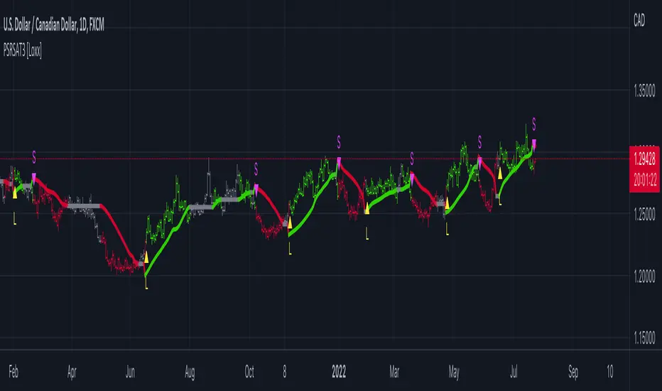
R-squared Adaptive T3 [Loxx]R-squared Adaptive T3 is an R-squared adaptive version of Tilson's T3 moving average. This adaptivity was originally proposed by mladen on various forex forums. This is considered experimental but shows how to use r-squared adapting methods to moving averages. In theory, the T3 is a six-pole non-linear Kalman filter.
What is the T3 moving average?
Better Moving Averages Tim Tillson
November 1, 1998
Tim Tillson is a software project manager at Hewlett-Packard, with degrees in Mathematics and Computer Science. He has privately traded options and equities for 15 years.
Introduction
"Digital filtering includes the process of smoothing, predicting, differentiating, integrating, separation of signals, and removal of noise from a signal. Thus many people who do such things are actually using digital filters without realizing that they are; being unacquainted with the theory, they neither understand what they have done nor the possibilities of what they might have done."
This quote from R. W. Hamming applies to the vast majority of indicators in technical analysis. Moving averages, be they simple, weighted, or exponential, are lowpass filters; low frequency components in the signal pass through with little attenuation, while high frequencies are severely reduced.
"Oscillator" type indicators (such as MACD, Momentum, Relative Strength Index) are another type of digital filter called a differentiator.
Tushar Chande has observed that many popular oscillators are highly correlated, which is sensible because they are trying to measure the rate of change of the underlying time series, i.e., are trying to be the first and second derivatives we all learned about in Calculus.
We use moving averages (lowpass filters) in technical analysis to remove the random noise from a time series, to discern the underlying trend or to determine prices at which we will take action. A perfect moving average would have two attributes:
It would be smooth, not sensitive to random noise in the underlying time series. Another way of saying this is that its derivative would not spuriously alternate between positive and negative values.
It would not lag behind the time series it is computed from. Lag, of course, produces late buy or sell signals that kill profits.
The only way one can compute a perfect moving average is to have knowledge of the future, and if we had that, we would buy one lottery ticket a week rather than trade!
Having said this, we can still improve on the conventional simple, weighted, or exponential moving averages. Here's how:
Two Interesting Moving Averages
We will examine two benchmark moving averages based on Linear Regression analysis.
In both cases, a Linear Regression line of length n is fitted to price data.
I call the first moving average ILRS, which stands for Integral of Linear Regression Slope. One simply integrates the slope of a linear regression line as it is successively fitted in a moving window of length n across the data, with the constant of integration being a simple moving average of the first n points. Put another way, the derivative of ILRS is the linear regression slope. Note that ILRS is not the same as a SMA (simple moving average) of length n, which is actually the midpoint of the linear regression line as it moves across the data.
We can measure the lag of moving averages with respect to a linear trend by computing how they behave when the input is a line with unit slope. Both SMA(n) and ILRS(n) have lag of n/2, but ILRS is much smoother than SMA.
Our second benchmark moving average is well known, called EPMA or End Point Moving Average. It is the endpoint of the linear regression line of length n as it is fitted across the data. EPMA hugs the data more closely than a simple or exponential moving average of the same length. The price we pay for this is that it is much noisier (less smooth) than ILRS, and it also has the annoying property that it overshoots the data when linear trends are present.
However, EPMA has a lag of 0 with respect to linear input! This makes sense because a linear regression line will fit linear input perfectly, and the endpoint of the LR line will be on the input line.
These two moving averages frame the tradeoffs that we are facing. On one extreme we have ILRS, which is very smooth and has considerable phase lag. EPMA has 0 phase lag, but is too noisy and overshoots. We would like to construct a better moving average which is as smooth as ILRS, but runs closer to where EPMA lies, without the overshoot.
A easy way to attempt this is to split the difference, i.e. use (ILRS(n)+EPMA(n))/2. This will give us a moving average (call it IE/2) which runs in between the two, has phase lag of n/4 but still inherits considerable noise from EPMA. IE/2 is inspirational, however. Can we build something that is comparable, but smoother? Figure 1 shows ILRS, EPMA, and IE/2.
Filter Techniques
Any thoughtful student of filter theory (or resolute experimenter) will have noticed that you can improve the smoothness of a filter by running it through itself multiple times, at the cost of increasing phase lag.
There is a complementary technique (called twicing by J.W. Tukey) which can be used to improve phase lag. If L stands for the operation of running data through a low pass filter, then twicing can be described by:
L' = L(time series) + L(time series - L(time series))
That is, we add a moving average of the difference between the input and the moving average to the moving average. This is algebraically equivalent to:
2L-L(L)
This is the Double Exponential Moving Average or DEMA, popularized by Patrick Mulloy in TASAC (January/February 1994).
In our taxonomy, DEMA has some phase lag (although it exponentially approaches 0) and is somewhat noisy, comparable to IE/2 indicator.
We will use these two techniques to construct our better moving average, after we explore the first one a little more closely.
Fixing Overshoot
An n-day EMA has smoothing constant alpha=2/(n+1) and a lag of (n-1)/2.
Thus EMA(3) has lag 1, and EMA(11) has lag 5. Figure 2 shows that, if I am willing to incur 5 days of lag, I get a smoother moving average if I run EMA(3) through itself 5 times than if I just take EMA(11) once.
This suggests that if EPMA and DEMA have 0 or low lag, why not run fast versions (eg DEMA(3)) through themselves many times to achieve a smooth result? The problem is that multiple runs though these filters increase their tendency to overshoot the data, giving an unusable result. This is because the amplitude response of DEMA and EPMA is greater than 1 at certain frequencies, giving a gain of much greater than 1 at these frequencies when run though themselves multiple times. Figure 3 shows DEMA(7) and EPMA(7) run through themselves 3 times. DEMA^3 has serious overshoot, and EPMA^3 is terrible.
The solution to the overshoot problem is to recall what we are doing with twicing:
DEMA(n) = EMA(n) + EMA(time series - EMA(n))
The second term is adding, in effect, a smooth version of the derivative to the EMA to achieve DEMA. The derivative term determines how hot the moving average's response to linear trends will be. We need to simply turn down the volume to achieve our basic building block:
EMA(n) + EMA(time series - EMA(n))*.7;
This is algebraically the same as:
EMA(n)*1.7-EMA(EMA(n))*.7;
I have chosen .7 as my volume factor, but the general formula (which I call "Generalized Dema") is:
GD(n,v) = EMA(n)*(1+v)-EMA(EMA(n))*v,
Where v ranges between 0 and 1. When v=0, GD is just an EMA, and when v=1, GD is DEMA. In between, GD is a cooler DEMA. By using a value for v less than 1 (I like .7), we cure the multiple DEMA overshoot problem, at the cost of accepting some additional phase delay. Now we can run GD through itself multiple times to define a new, smoother moving average T3 that does not overshoot the data:
T3(n) = GD(GD(GD(n)))
In filter theory parlance, T3 is a six-pole non-linear Kalman filter. Kalman filters are ones which use the error (in this case (time series - EMA(n)) to correct themselves. In Technical Analysis, these are called Adaptive Moving Averages; they track the time series more aggressively when it is making large moves.
Included:
Bar coloring
Signals
Alerts
Loxx's Expanded Source Types
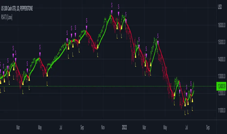
Multi-Indicator by johntradingwickThe Multi-Indicator includes the functionality of the following indicators:
1. Market Structure
2. Support and Resistance
3. VWAP
4. Simple Moving Average
5. Exponential Moving Average
Functionality of the Multi-Indicator:
Market Structure
As we already know, the market structure is one of the most important things in trading. If we are able to identify the trend correctly, it takes away a huge burden. For this, I have used the Zig Zag indicator to identify price trends. It plots points on the chart whenever the prices reverse by a larger percentage than a predetermined variable. The points are then connected by straight lines that will help you to identify the swing high and low.
This will help you to filter out any small price movements, making it easier to identify the trend, its direction, and its strength levels. You can change the period in consideration and the deviation by changing the deviation % and the depth.
Support and Resistance
The indicator provides the functionality to add support and resistance levels. If you want more levels just change the timeframe it looks at in the settings. It will pull the SR levels off the timeframe specified in the settings.
You can select the timeframe for support and resistance levels. The default time frame is “same as the chart”.
You can also extend lines to the right and change the width and colour of the lines. There is also an option to change the criteria to select the lines as valid support or resistance. You can extend the S/R level or use the horizontal lines to mark the level when there is a change in polarity.
VWAP
Volume Weighted Average Price (VWAP) is used to measure the average price weighted by volume. VWAP is typically used with intraday charts as a way to determine the general direction of intraday prices. It's similar to a moving average in that when the price is above VWAP, prices are rising and when the price is below VWAP, prices are falling. VWAP is primarily used by technical analysts to identify market trend.
Simple Moving Average
A simple Moving Average is an unweighted Moving Average. This means that each day in the data set has equal importance and is weighted equally. As each new day ends, the oldest data point is dropped and the newest one is added to the beginning.
The multi-indicator has the ability to provide 5 moving averages. This is particularly helpful if you want to use various time periods such as 20, 50, 100, and 200. Although this is just basic functionality, it comes in handy if you are using a free account.
Exponential Moving Average
An exponential moving average (EMA) is a type of moving average (MA) that places a greater weight and significance on the most recent data points. An exponentially weighted moving average reacts more significantly to recent price changes than a simple moving average. The multi-indicator provides 5 exponential moving averages. This is particularly helpful if you want to use various time periods such as 20, 50, 100, and 200.
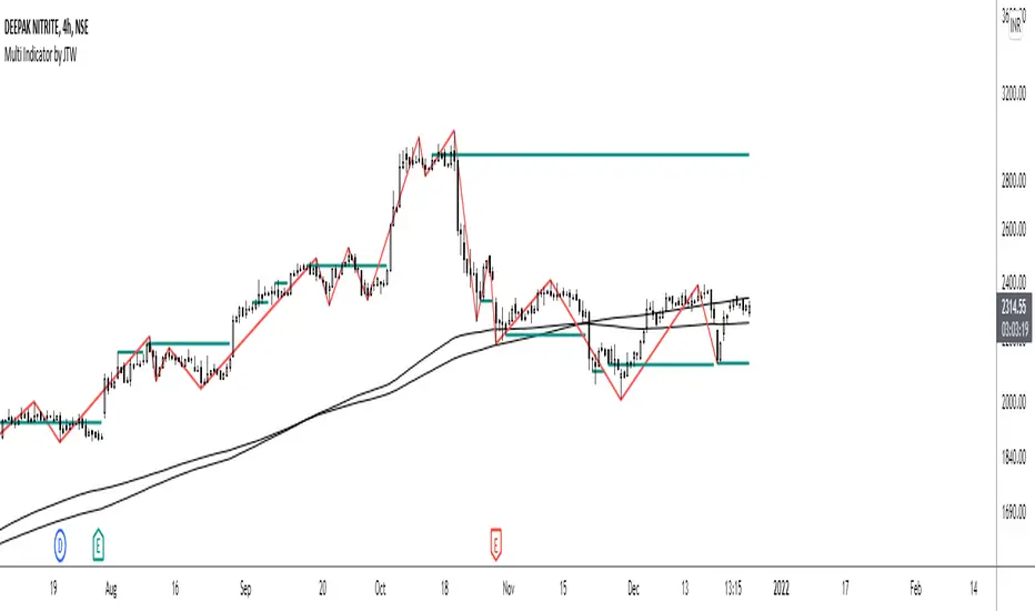
paigep.llc - SuperMA
SuperMA is a multi-layered moving-average and candle-coloring system that combines SMA, EMA, and optional HMA logic to help traders visualize trend shifts, pullbacks, and momentum changes in a clean, structured way.
The script includes multiple modules: trend-based moving averages, pullback signals, exit logic, and an optional HMA cross engine.
📌 Core Features
1. Full SMA + EMA Framework
The indicator plots multiple moving averages (8, 9, 13, 20, 50, 200) using both SMA and EMA calculations. Each line automatically colors bullish or bearish based on its relationship to the 200-period baseline. Users can toggle SMAs and EMAs independently for clearer chart control.
2. Main Trend Entry & Exit Logic (8×200 and 8×20)
Built-in crossover logic detects:
Main Entry: SMA 8 crossing above/below EMA 200
Main Exit: SMA 8 and SMA 20 cross (with an option to choose which SMA is treated as the “fast” leg)
A “first exit only” option allows the script to ignore additional exit signals until a new trend regime begins.
3. Pullback Module (20 SMA Interaction)
Pullback entries and exits occur when price crosses the 20 SMA during existing trend conditions.
This includes:
Pullback entries through the 20 SMA
Pullback exits back across the 20 SMA
Labels and candle colors are available for all pullback events.
4. Optional HMA Cross Module
A separate module allows traders to use two Hull Moving Averages (HMA) with customizable:
Lengths
Independent timeframes
Line colors
Cross-based entries and exits
This module has its own events, labels, and optional candle coloring.
5. Advanced Candle Coloring System
Candle coloring is layered in priority order, based on:
Main trend entries
Main exits
HMA entries
HMA exits
Pullback entries
Pullback exits
Trend-only candles (based on SMA 8 relative to EMA 200)
Users may also independently color wicks and borders.
6. Configurable Alerts (Fully Decoupled from Visuals)
Alerts are available for all major events, including:
Main Entries (8×200)
Main Exits (8×20)
Pullback Entries and Exits
HMA Entries and Exits
Bull or Bear Trend candles
Any colored candle event
Alerts can fire on bar close only or intrabar, depending on user preference.
Use Cases
SuperMA helps traders visualize:
Trend direction using SMA/EMA structure
Momentum shifts through HMA crosses
Pullback zones around the 20 SMA
Early regime transitions based on the 8×200 relationship
Candle-level context through color-coded bars
The indicator works across all markets and timeframes.
⚠️ Note
This tool is for visual and analytical assistance only. It does not guarantee future performance and should be combined with additional analysis and risk management.

Michal D. Lagless Moving Average | MisinkoMasterThe 𝕸𝖎𝖈𝖍𝖆𝖑 𝕯. 𝕷𝖆𝖌𝖑𝖊𝖘𝖘 𝕸𝖔𝖛𝖎𝖓𝖌 𝕬𝖛𝖊𝖗𝖆𝖌𝖊 is my latest creation of a trend following tool, which is a bit different from the rest. By trying to de-lag the classical moving average, it gives you fast signals on changes in trend as fast as possible, keeping traders & investors always in check for potential risks they might want to avoid.
How does it work?
First we need to calculate lengths. The lengths are calcuted using a user defined input called the "Length Multiplier" and we of course need as well the length input too.
The indicator uses 10 lengths, 5 for an average price, 5 for median price.
The length for the average is the following:
length_2_avg = length_1_avg * length_multiplier
length_3_avg = length_2_avg * length_multiplier
...
and for the median lengths:
length_1_median = length_2_avg
length_2_median = length_3_avg
Here applies this rule
length_x_median < length_x_avg
This is intentional, and it is because the average is a little more reactive, while the median is a bit slower. To make up for the "slowness" of the median, we simple reduce the length of it a bit more than the average.
Now that we have our length we are ready to calculate averages and medians over their respective period. This is the a normal average from elementary school, nothing too fancy.
Now that we have all of them we match the pairs using another user defined input called "Median Weight" like so:
(Average_x * (2-median_weight) + Median_x * median_weight)/2
This gives more weight to the average (also due to the max value limit set to avoid breaking the fundational logic behind it).
After doing it to all the pairs we now average those pairs using another input called "Exponential Weight Multiplier".
The Exponential Weight Multiplier is used for weights which I will cover soon:
weight1 = weight
weight2 = weight * weight
weight3 = weight * weight * weight....
This is done until we have all the weights calculated
This gives exponentially more weight to the less lagging indicators, which is how we delag the indicator.
Then we sum all the pairs like so:
sum = pair1 * weight1 + pair2 * weight2 + pair3 * weight3 + pair4 * weight4 + pair5 * weight5
Then the sum is divided by the sum of weights, this results in us getting the final value.
Methodology & What is the actual point & how was it made?
I want to cover this one a bit deeper:
The methodology behind this was creating an indicator that would not be lagging, and would be able to avoid lag while not producing signals too often.
In many attempts in the first part, I tried using EMA, RMA, DEMA, TEMA, HMA, SMA and so on, but they were too noisy (except for SMA & RMA, but those had their flaws), so I tried the classical average taught in elementary school. This one worked better, but the noise was too high still after all this time. This made me include the median, which helped the noise, but made it far too lagging.
Here came the idea of making the median length lower and adding weights to counter the lag of the median, but it was still too lagging. This made me make the weights for lengths more exponential, while previously they were calculated using a little bit amplified sums that were alright, but nowhere near my desired result.
Using the new weights I got further, and after a bit of testing I was sattisfied with the results.
The logic for the trend was a big part in my development part, there were many I could think of, but not enough time to try them, so I stuck to the usual one, and I leave it up to YOU to beat my trend logic and get even better results.
Use Cases:
- Price/MA Crossovers
Simple, effective, useful
- Source for other indicators
This I tried myself, and it worked in a cool way, making the signals of for example RSI much smoother, so definitely try it out if you know how to code, or just simply put it in the source of the RSI.
- ROC
This trend logic stuck with me, I think you could find a way to make it good, but mainly for the people that can code in pine, trying out to combine the trend logic with ROC could work very well, do not sleep on it!
- Education
This concept is not really that complex, so for people looking for new ideas, inspiration, or just watching how trend following tools behave in general this is something that could benefit anyone, as the concept can be applied to ANYTHING, even the classical RSI, MACD, you could try even the Parabolic SAR, maybe STC or VZO, there is no limit to imagination.
- Strategy creation
Filtering this indicator with "and" conditions, or maybe even "or" or anything really could be very useful in a strategy that desires fast signals.
- Price Distance from bands
I noticed this while looking at past performance:
The stronger the trend the higher the distance from the Moving Average.
Final Notes
Watch out for mean reverting markets, as this is trend following you could get easily screwed in them.
Play around with this if it fits your desired outcome, you might find something I did not.
Hope you find it useful,
See you next time!
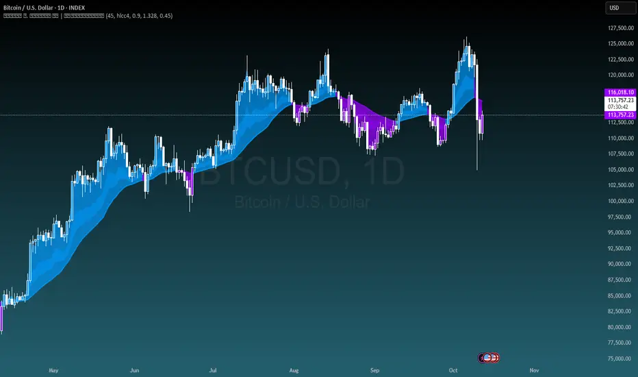
T3 [DCAUT]█ T3
📊 INDICATOR OVERVIEW
The T3 Moving Average is a smoothing indicator developed by Tim Tillson and published in Technical Analysis of Stocks & Commodities magazine (January 1998). The algorithm applies Generalized DEMA (Double Exponential Moving Average) recursively three times, creating a six-pole filtering effect that aims to balance noise reduction with responsiveness while minimizing lag relative to price changes.
📐 MATHEMATICAL FOUNDATION
Generalized DEMA (GD) Function:
The core building block is the Generalized DEMA function, which combines two exponential moving averages with weights controlled by the volume factor:
GD(input, v) = EMA(input) × (1 + v) - EMA(EMA(input)) × v
Where v is the volume factor parameter (default 0.7). This weighted combination reduces lag while maintaining smoothness by extrapolating beyond the first EMA using the double-smoothed EMA as a reference.
T3 Calculation Process:
T3 applies the GD function three times recursively:
T3 = GD(GD(GD(Price, v), v), v)
This triple nesting creates a six-pole smoothing effect (each GD applies two EMA operations, resulting in 2 × 3 = 6 total EMA calculations). The cascading refinement progressively filters noise while preserving trend information.
Step-by-Step Breakdown:
First GD application: GD1 = EMA(Price) × (1 + v) - EMA(EMA(Price)) × v - Creates initial smoothed series with lag reduction
Second GD application: GD2 = EMA(GD1) × (1 + v) - EMA(EMA(GD1)) × v - Further refines the smoothing while maintaining responsiveness
Third GD application: T3 = EMA(GD2) × (1 + v) - EMA(EMA(GD2)) × v - Final refinement produces the T3 output
Volume Factor Impact:
The volume factor (v) is the key parameter controlling the balance between smoothness and responsiveness. Tim Tillson recommended v = 0.7 as the optimal default value.
Lower volume factors (v closer to 0.0): Increase the extrapolation effect, making T3 more responsive to price changes but potentially more sensitive to noise.
Higher volume factors (v closer to 1.0): Reduce the extrapolation effect, producing smoother output with less sensitivity to short-term fluctuations but slightly more lag.
The recursive application of the volume factor through three GD stages creates a nonlinear filtering effect that achieves superior lag reduction compared to traditional moving averages of equivalent smoothness.
📊 SIGNAL INTERPRETATION
Trend Direction Signals:
Green Line (T3 Rising): Smoothed trend line is rising, may indicate uptrend, consider bullish opportunities when confirmed by other factors
Red Line (T3 Falling): Smoothed trend line is falling, may indicate downtrend, consider bearish opportunities when confirmed by other factors
Gray Line (T3 Flat): Smoothed trend line is flat, indicates unclear trend or consolidation phase
Price Crossover Signals:
Price Crosses Above T3: Price breaks above smoothed trend line, may be bullish signal, requires confirmation from other indicators
Price Crosses Below T3: Price breaks below smoothed trend line, may be bearish signal, requires confirmation from other indicators
Price Position Relative to T3: Price sustained above T3 may indicate uptrend, sustained below may indicate downtrend
Supporting Analysis Signals:
T3 Slope Angle: Steeper slopes indicate stronger trend momentum, flatter slopes suggest weakening trends
Price Deviation: Significant price separation from T3 may indicate overextension, watch for pullback or reversal
Dynamic Support/Resistance: T3 line can serve as dynamic support (in uptrends) or resistance (in downtrends) reference
🎯 STRATEGIC APPLICATIONS
Common Usage Patterns:
The T3 Moving Average can be incorporated into trading analysis in various ways. These represent common approaches used by market participants, though effectiveness varies by market conditions and requires individual testing:
Trend Filtering:
T3 can be used as a trend filter by observing the relationship between price and the T3 line. The color-coded slope (green for rising, red for falling, gray for sideways) provides visual feedback about the current trend direction of the smoothed series.
Price Crossover Analysis:
Some traders monitor crossovers between price and the T3 line as potential indication points. When price crosses the T3 line, it may suggest a change in the relationship between current price action and the smoothed trend.
Multi-Timeframe Observation:
T3 can be applied to multiple timeframes simultaneously. Observing alignment or divergence between different timeframe T3 indicators may provide context about trend consistency across time scales.
Dynamic Reference Level:
The T3 line can serve as a dynamic reference level for price action analysis. Price distance from T3, price reactions when approaching T3, and the behavior of price relative to the T3 line can all be incorporated into market analysis frameworks.
Application Considerations:
Any trading application should be thoroughly tested on historical data before implementation
T3 performance characteristics vary across different market conditions and asset types
The indicator provides smoothed trend information but does not predict future price movements
Combining T3 with other analytical tools and market context improves analysis quality
Risk management practices remain essential regardless of the analytical approach used
📋 DETAILED PARAMETER CONFIGURATION
Source Selection:
Close Price (Default): Standard choice for end-of-period trend analysis, reduces intrabar noise
HL2 (High+Low)/2: Provides balanced view of price action, considers full bar range
HLC3 or OHLC4: Incorporates more price information, may provide smoother results
Selection Impact: Different sources affect signal timing and smoothness characteristics
Length Configuration:
Shorter periods: More responsive, faster reaction, frequent signals, but higher false signal risk in choppy markets
Longer periods: Smoother output, fewer signals, better for long-term trends, but slower response
Default 14 periods is a common baseline, but optimal length varies by asset, timeframe, and market conditions
Parameter selection should be determined through backtesting rather than general recommendations
Volume Factor Configuration:
Lower values (closer to 0.0): Increase responsiveness but also noise sensitivity
Higher values (closer to 1.0): Increase smoothness but slightly more lag
Default 0.7 (Tim Tillson's recommendation) provides good balance for most applications
Optimal value depends on signal frequency versus reliability preference, test for specific use case
Parameter Optimization Approach:
There are no universal "best" parameter values - optimal settings depend on the specific asset, timeframe, market regime, and trading strategy
Start with default values (Length: 14, Volume Factor: 0.7) and adjust based on observed performance in your target market
Conduct systematic backtesting across different market conditions to evaluate parameter sensitivity
Consider that parameters optimized for historical data may not perform identically in future market conditions
Monitor performance and be prepared to adjust parameters as market characteristics evolve
📈 DESIGN FEATURES & MARKET ADAPTATION
Algorithm Design Features:
Simple Moving Average (SMA): Equal weighting across lookback period
Exponential Moving Average (EMA): Exponentially decreasing weights on historical prices
T3 Moving Average: Recursive Generalized DEMA with adjustable volume factor
Market Condition Adaptation:
Trending markets: Smoothed indicators generally align more closely with sustained directional movement
Ranging markets: All moving averages may generate more crossover signals during non-trending periods
Volatile conditions: Higher smoothing parameters reduce short-term sensitivity but increase lag
Indicator behavior relative to market conditions should be evaluated for specific applications
USAGE NOTES
This indicator is designed for technical analysis and educational purposes. The T3 Moving Average has limitations and should not be used as the sole basis for trading decisions. Like all trend-following indicators, its performance varies with market conditions, and past signal characteristics do not guarantee future results.
Key Points:
T3 is a lagging indicator that responds to price changes rather than predicting future movements
Signals should be confirmed with other technical tools and market context
Parameters should be optimized for specific market and timeframe
Risk management and position sizing are essential
Market regime changes can affect indicator effectiveness
Test strategies thoroughly on historical data before live implementation
Consider broader market context and fundamental factors
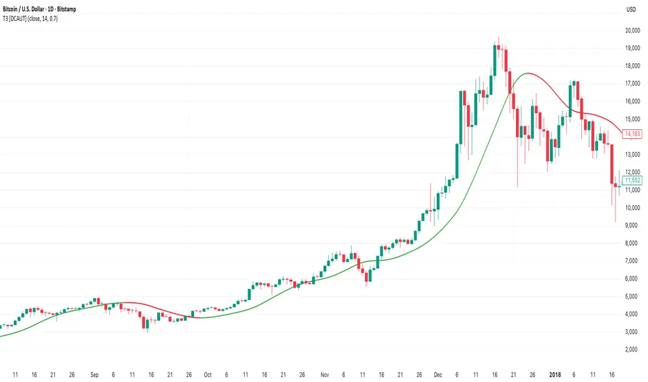
Time-Decaying Percentile Oscillator [BackQuant]Time-Decaying Percentile Oscillator
1. Big-picture idea
Traditional percentile or stochastic oscillators treat every bar in the look-back window as equally important. That is fine when markets are slow, but if volatility regime changes quickly yesterday’s print should matter more than last month’s. The Time-Decaying Percentile Oscillator attempts to fix that blind spot by assigning an adjustable weight to every past price before it is ranked. The result is a percentile score that “breathes” with market tempo much faster to flag new extremes yet still smooth enough to ignore random noise.
2. What the script actually does
Build a weight curve
• You pick a look-back length (default 28 bars).
• You decide whether weights fall Linearly , Exponentially , by Power-law or Logarithmically .
• A decay factor (lower = faster fade) shapes how quickly the oldest price loses influence.
• The array is normalised so all weights still sum to 1.
Rank prices by weighted mass
• Every close in the window is paired with its weight.
• The pairs are sorted from low to high.
• The cumulative weight is walked until it equals your chosen percentile level (default 50 = median).
• That price becomes the Time-Decayed Percentile .
Find dispersion with robust statistics
• Instead of a fragile standard deviation the script measures weighted Median-Absolute-Deviation about the new percentile.
• You multiply that deviation by the Deviation Multiplier slider (default 1.0) to get a non-parametric volatility band.
Build an adaptive channel
• Upper band = percentile + (multiplier × deviation)
• Lower band = percentile – (multiplier × deviation)
Normalise into a 0-100 oscillator
• The current close is mapped inside that band:
0 = lower band, 50 = centre, 100 = upper band.
• If the channel squeezes, tiny moves still travel the full scale; if volatility explodes, it automatically widens.
Optional smoothing
• A second-stage moving average (EMA, SMA, DEMA, TEMA, etc.) tames the jitter.
• Length 22 EMA by default—change it to tune reaction speed.
Threshold logic
• Upper Threshold 70 and Lower Threshold 30 separate standard overbought/oversold states.
• Extreme bands 85 and 15 paint background heat when aggressive fade or breakout trades might trigger.
Divergence engine
• Looks back twenty bars.
• Flags Bullish divergence when price makes a lower low but oscillator refuses to confirm (value < 40).
• Flags Bearish divergence when price prints a higher high but oscillator stalls (value > 60).
3. Component walk-through
• Source – Any price series. Close by default, switch to typical price or custom OHLC4 for futures spreads.
• Look-back Period – How many bars to rank. Short = faster, long = slower.
• Base Percentile Level – 50 shows relative position around the median; set to 25 / 75 for quartile tracking or 90 / 10 for extreme tails.
• Deviation Multiplier – Higher values widen the dynamic channel, lowering whipsaw but delaying signals.
• Decay Settings
– Type decides the curve shape. Exponential (default 1.16) mimics EMA logic.
– Factor < 1 shrinks influence faster; > 1 spreads influence flatter.
– Toggle Enable Time Decay off to compare with classic equal-weight stochastic.
• Smoothing Block – Choose one of seven MA flavours plus length.
• Thresholds – Overbought / Oversold / Extreme levels. Push them out when working on very mean-reverting assets like FX; pull them in for trend monsters like crypto.
• Display toggles – Show or hide threshold lines, extreme filler zones, bar colouring, divergence labels.
• Colours – Bullish green, bearish red, neutral grey. Every gradient step is automatically blended to generate a heat map across the 0-100 range.
4. How to read the chart
• Oscillator creeping above 70 = market auctioning near the top of its adaptive range.
• Fast poke above 85 with no follow-through = exhaustion fade candidate.
• Slow grind that lives above 70 for many bars = valid bullish trend, not a fade.
• Cross back through 50 shows balance has shifted; treat it like a micro trend change.
• Divergence arrows add extra confidence when you already see two-bar reversal candles at range extremes.
• Background shading (semi-transparent red / green) warns of extreme states and throttles your position size.
5. Practical trading playbook
Mean-reversion scalps
1. Wait for oscillator to reach your desired OB/ OS levels
2. Check the slope of the smoothing MA—if it is flattening the squeeze is mature.
3. Look for a one- or two-bar reversal pattern.
4. Enter against the move; first target = midline 50, second target = opposite threshold.
5. Stop loss just beyond the extreme band.
Trend continuation pullbacks
1. Identify a clean directional trend on the price chart.
2. During the trend, TDP will oscillate between midline and extreme of that side.
3. Buy dips when oscillator hits OS levels, and the same for OB levels & shorting
4. Exit when oscillator re-tags the same-side extreme or prints divergence.
Volatility regime filter
• Use the Enable Time Decay switch as a regime test.
• If equal-weight oscillator and decayed oscillator diverge widely, market is entering a new volatility regime—tighten stops and trade smaller.
Divergence confirmation for other indicators
• Pair TDP divergence arrows with MACD histogram or RSI to filter false positives.
• The weighted nature means TDP often spots divergence a bar or two earlier than standard RSI.
Swing breakout strategy
1. During consolidation, band width compresses and oscillator oscillates around 50.
2. Watch for sudden expansion where oscillator blasts through extreme bands and stays pinned.
3. Enter with momentum in breakout direction; trail stop behind upper or lower band as it re-expands.
6. Customising decay mathematics
Linear – Each older bar loses the same fixed amount of influence. Intuitive and stable; good for slow swing charts.
Exponential – Influence halves every “decay factor” steps. Mirrors EMA thinking and is fastest to react.
Power-law – Mid-history bars keep more authority than exponential but oldest data still fades. Handy for commodities where seasonality matters.
Logarithmic – The gentlest curve; weight drops sharply at first then levels off. Mimics how traders remember dramatic moves for weeks but forget ordinary noise quickly.
Turn decay off to verify the tool’s added value; most users never switch back.
7. Alert catalogue
• TD Overbought / TD Oversold – Cross of regular thresholds.
• TD Extreme OB / OS – Breach of danger zones.
• TD Bullish / Bearish Divergence – High-probability reversal watch.
• TD Midline Cross – Momentum shift that often precedes a window where trend-following systems perform.
8. Visual hygiene tips
• If you already plot price on a dark background pick Bullish Color and Bearish Color default; change to pastel tones for light themes.
• Hide threshold lines after you memorise the zones to declutter scalping layouts.
• Overlay mode set to false so the oscillator lives in its own panel; keep height about 30 % of screen for best resolution.
9. Final notes
Time-Decaying Percentile Oscillator marries robust statistical ranking, adaptive dispersion and decay-aware weighting into a simple oscillator. It respects both recent order-flow shocks and historical context, offers granular control over responsiveness and ships with divergence and alert plumbing out of the box. Bolt it onto your price action framework, trend-following system or volatility mean-reversion playbook and see how much sooner it recognises genuine extremes compared to legacy oscillators.
Backtest thoroughly, experiment with decay curves on each asset class and remember: in trading, timing beats timidity but patience beats impulse. May this tool help you find that edge.

Targets For Many Indicators [LuxAlgo]The Targets For Many Indicators is a useful utility tool able to display targets for many built-in indicators as well as external indicators. Targets can be set for specific user-set conditions between two series of values, with the script being able to display targets for two different user-set conditions.
Alerts are included for the occurrence of a new target as well as for reached targets.
🔶 USAGE
Targets can help users determine the price limit where the price might start deviating from an indication given by one or multiple indicators. In the context of trading, targets can help secure profits/reduce losses of a trade, as such this tool can be useful to evaluate/determine user take profits/stop losses.
Due to these essentially being horizontal levels, they can also serve as potential support/resistances, with breakouts potentially confirming new trends.
In the above example, we set targets 3 ATR's away from the closing price when the price crosses over the script built-in SuperTrend indicator using ATR period 10 and factor 3. Using "Long Position Target" allows setting a target above the price, disabling this setting will place targets below the price.
Users might be interested in obtaining new targets once one is reached, this can be done by enabling "New Target When Reached" in the target logic setting section, resulting in more frequent targets.
Lastly, users can restrict new target creation until current ones are reached. This can result in fewer and longer-term targets, with a higher reach rate.
🔹 Dashboard
A dashboard is displayed on the top right of the chart, displaying the amount, reach rate of targets 1/2, and total amount.
This dashboard can be useful to evaluate the selected target distances relative to the selected conditions, with a higher reach rate suggesting the distance of the targets from the price allows them to be reached.
🔶 DETAILS
🔹 Indicators
Besides 'External' sources, each source can be set at 1 of the following Build-In Indicators :
ACCDIST : Accumulation/distribution index
ATR : Average True Range
BB (Middle, Upper or Lower): Bollinger Bands
CCI : Commodity Channel Index
CMO : Chande Momentum Oscillator
COG : Center Of Gravity
DC (High, Mid or Low): Donchian Channels
DEMA : Double Exponential Moving Average
EMA : Exponentially weighted Moving Average
HMA : Hull Moving Average
III : Intraday Intensity Index
KC (Middle, Upper or Lower): Keltner Channels
LINREG : Linear regression curve
MACD (macd, signal or histogram): Moving Average Convergence/Divergence
MEDIAN : median of the series
MFI : Money Flow Index
MODE : the mode of the series
MOM : Momentum
NVI : Negative Volume Index
OBV : On Balance Volume
PVI : Positive Volume Index
PVT : Price-Volume Trend
RMA : Relative Moving Average
ROC : Rate Of Change
RSI : Relative Strength Index
SMA : Simple Moving Average
STOCH : Stochastic
Supertrend
TEMA : Triple EMA or Triple Exponential Moving Average
VWAP : Volume Weighted Average Price
VWMA : Volume-Weighted Moving Average
WAD : Williams Accumulation/Distribution
WMA : Weighted Moving Average
WVAD : Williams Variable Accumulation/Distribution
%R : Williams %R
Each indicator is provided with a link to the Reference Manual or to the Build-In Indicators page.
The latter contains more information about each indicator.
Note that when "Show Source Values" is enabled, only values that can be logically found around the price will be shown. For example, Supertrend , SMA , EMA , BB , ... will be made visible. Values like RSI , OBV , %R , ... will not be visible since they will deviate too much from the price.
🔹 Interaction with settings
This publication contains input fields, where you can enter the necessary inputs per indicator.
Some indicators need only 1 value, others 2 or 3.
When several input values are needed, you need to separate them with a comma.
You can use 0 to 4 spaces between without a problem. Even an extra comma doesn't give issues.
The red colored help text will guide you further along (Only when Target is enabled)
Some examples that work without issues:
Some examples that work with issues:
As mentioned, the errors won't be visible when the concerning target is disabled
🔶 SETTINGS
Show Target Labels: Display target labels on the chart.
Candle Coloring: Apply candle coloring based on the most recent active target.
Target 1 and Target 2 use the same settings below:
Enable Target: Display the targets on the chart.
Long Position Target: Display targets above the price a user selected condition is true. If disabled will display the targets below the price.
New Target Condition: Conditional operator used to compare "Source A" and "Source B", options include CrossOver, CrossUnder, Cross, and Equal.
🔹 Sources
Source A: Source A input series, can be an indicator or external source.
External: External source if 'External" is selected in "Source A".
Settings: Settings of the selected indicator in "Source A", entered settings of indicators requiring multiple ones must be comma separated, for example, "10, 3".
Source B: Source B input series, can be an indicator or external source.
External: External source if 'External" is selected in "Source B".
Settings: Settings of the selected indicator in "Source B", entered settings of indicators requiring multiple ones must be comma separated, for example, "10, 3".
Source B Value: User-defined numerical value if "value" is selected in "Source B".
Show Source Values: Display "Source A" and "Source B" on the chart.
🔹 Logic
Wait Until Reached: When enabled will not create a new target until an existing one is reached.
New Target When Reached: Will create a new target when an existing one is reached.
Evaluate Wicks: Will use high/low prices to determine if a target is reached. Unselecting this setting will use the closing price.
Target Distance From Price: Controls the distance of a target from the price. Can be determined in currencies/points, percentages, ATR multiples, ticks, or using multiple of external values.
External Distance Value: External distance value when "External Value" is selected in "Target Distance From Price".
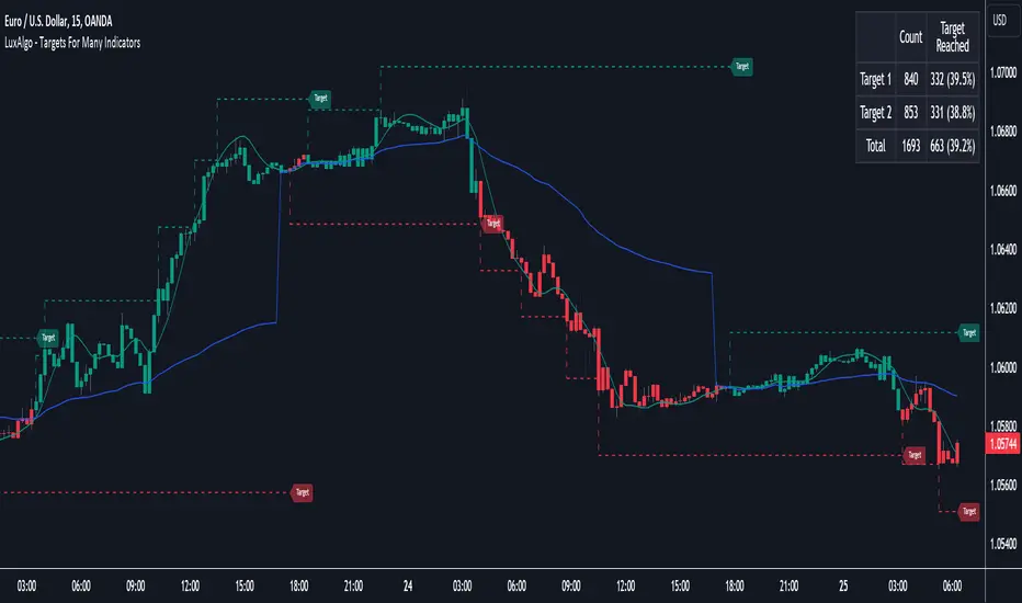
Parabolic Scalp Take Profit[ChartPrime]Indicators can be a great way to signal when the optimal time is for taking profits. However, many indicators are lagging in nature and will get market participants out of their trades at less than optimal price points. This take profit indicator uses the concept of slope and exponential gain to calculate when the optimal time is to take profits on your trades, thus making this a leading indicator.
Usage:
In essence the indicator will draw a parabolic line that starts from the market participants entry point and exponentially grows the slope of the line eventually intersecting with the price action. When price intersects with the parabolic line a take profit signal will appear in the form of an x. We have found that this take profit indicator is especially useful for scalp trades on lower timeframes.
How To Use:
Add the indicator to the chart. Click on the candle which the trade is on. Click on either the price which the trade will be at, or at the bottom of the candle in a long, or the top of a candle in a short. Select long or short. Open the settings of the indicator and adjust the aggressiveness to the desired value.
Settings:
- Start Time -- This is the bar in which your entry will be at, or occured at and the script will ask you to click on the bar with your mouse upon first adding the script.
- Start Price -- This is the price in which the entry will be at, or was at and the script will ask you to click on the price with your mouse upon first adding the script.
- Long/Short -- This is a setting which lets the script know if it is a long or a short trade, and the script will ask you to confirm this upon first adding it to the chart.
- Aggressiveness -- This directly affects how aggressive the exponential curve is. A value of 101 is the lowest possible setting, indicating a very non-aggressive exponential buildup. A value of 200 is the highest and most aggressive setting, indicating a doubling effect per bar on the slope.

EMAs DistancesThis indicator shows 4 configurable EMAs and the distances (values and percentages) to the last price of the stock, etf or index.
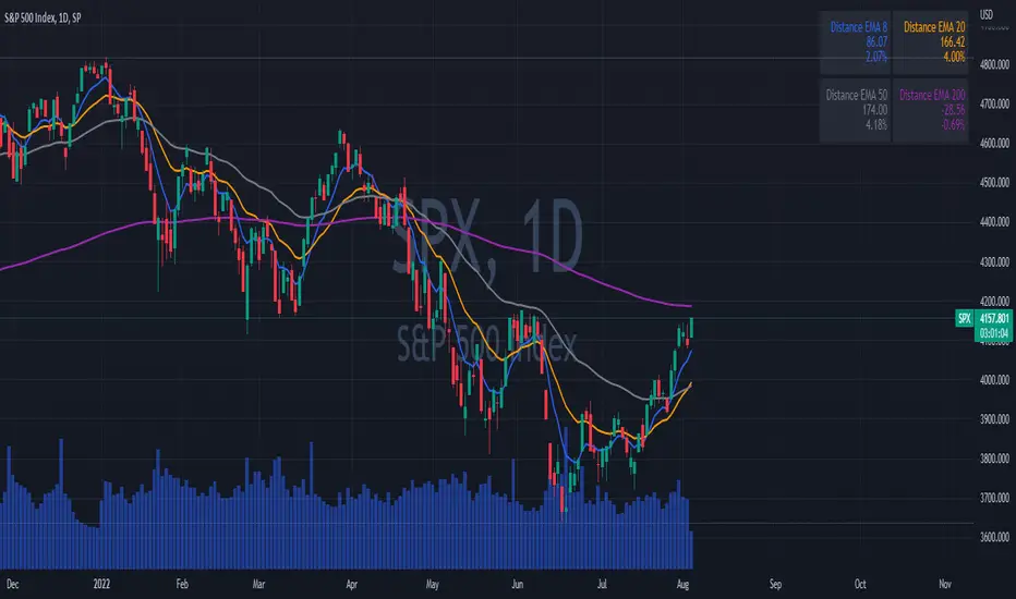
EMA PredictionThis script predicts future EMA values assuming that the price remains as configured (-50% to +50%).
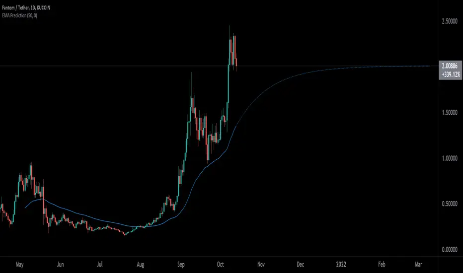
[blackcat] L1 New TRIX ScalperNOTE: Because the originally released script failed to comply with the House Rule in the description, it was banned. After revising and reviewing the description, it is republished again. Please forgive the inconvenience caused.
Level: 1
Background
The Triple Exponential Moving Average (TRIX) indicator is a strong technical analysis tool. It can help investors determine the price momentum and identify oversold and overbought signals in a financial asset. Jack Hutson is the creator of the TRIX indicator . He created it in the early 1980s to show the rate of change in a triple exponentially smoothed moving average.
When used as an oscillator, it shows a potential peak and trough price zones. A positive value tells traders that there is an overbought market while a negative value means an oversold market. When traders use TRIX as a momentum indicator, it filters spikes in the price that are vital to the general dominant trend.
A positive value means momentum is rising while a negative value means that momentum is reducing. A lot of analysts believe that when the TRIX crosses above the zero line it produces a buy signal, and when it closes below the zero line, it produces a sell signal.The indicator has three major components:
Zero line
TRIX line (or histograms)
Percentage Scale
Function
The TRIX indicator determines overbought and oversold markets, and it can also be a momentum indicator. Just as it is with most oscillators, TRIX oscillates around a zero line. Additionally, divergences between price and TRIX can mean great turning points in the market. TRIX calculates a triple exponential moving average of the log of the price input. It calculates this based on the time specified by the length input for the current bar.
Trading TRIX indicator signals
Zero line cross
TRIX can help determine the impulse of the market. With the 0 value acting as a centerline, if it crosses from below, it will be mean that the impulse is growing in the market.Traders can, therefore, look for opportunities to place buy orders in the market. Similarly, a cross of the centerline from above will mean a shrinking impulse in the market. Traders can, therefore, look for opportunities to sell in the market.
Signal line cross
To select the best entry points, investors add a signal line on the TRIX indicator. The signal line is a moving average of the TRIX indicator, and due to this, it will lag behind the TRIX.A signal to place a buy order will occur when the TRIX crosses the signal line from below. In the same way, a signal to place a sell order will come up when the TRIX crosses the signal line from above. This is applicable in both trending and ranging markets.In trending markets, a signal line cross will indicate an end of the price retracement, and the main trend will resume. In ranging markets, a signal line confirms that resistance and support zones have been upheld in the market.
Divergences
Traders can use the Triple Exponential Average can to identify when important turning points can happen in the market. They can achieve this by looking at divergences. Divergences happen when the price is moving in the opposite direction as the TRIX indicator.When price makes higher highs but the TRIX makes lower highs, it means that the up-trend is weakening, and a bearish reversal is about to form. When the price makes lower lows, but the TRIX makes higher lows, it means that a bullish reversal is about to happen. Bullish and bearish divergences happen when the security and the indicator do not confirm themselves. A bullish divergence can happen when the security makes a lower low, but the indicator forms a higher low. This higher low means less downside momentum that may foreshadow a bullish reversal. A bearish divergence happens when the commodity makes a higher low, but the indicator forms a lower high. This lower high indicates weak upside momentum that can foreshadow a bearish reversal sometimes. Bearish divergences do not work well in strong uptrends. Even though momentum appears to be weakening due to the indicator is making lower highs, momentum still has a bullish bias as long as it is above its centerline.When bullish and bearish divergences work, they work very well. The secret is to separate the bad signals from the good signals.
Key Signal
RXval --> new TRIX indicator.
AvgTRX --> linear regression average of new TRIX indicator.
Remarks
This is a Level 1 free and open source indicator.
Feedbacks are appreciated.
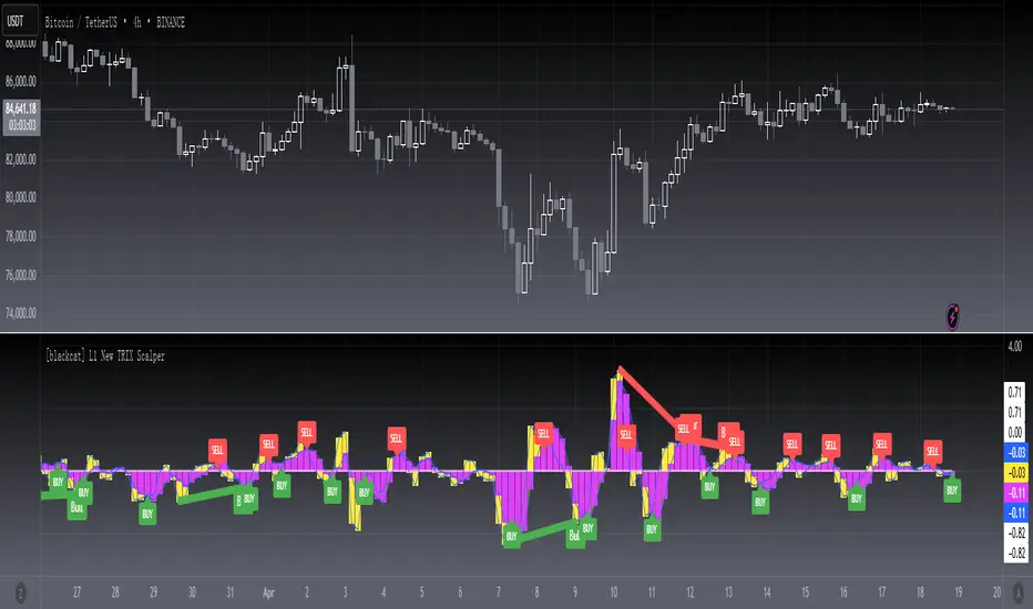
Resampling Filter Pack [DW]This is an experimental study that calculates filter values at user defined sample rates.
This study is aimed to provide users with alternative functions for filtering price at custom sample rates.
First, source data is resampled using the desired rate and cycle offset. The highest possible rate is 1 bar per sample (BPS).
There are three resampling methods to choose from:
-> BPS - Resamples based on the number of bars.
-> Interval - Resamples based on time in multiples of current charting timeframe.
-> PA - Resamples based on changes in price action by a specified size. The PA algorithm in this script is derived from my Range Filter algorithm.
The range for PA method can be sized in points, pips, ticks, % of price, ATR, average change, and absolute quantity.
Then, the data is passed through one of my custom built filter functions designed to calculate filter values upon trigger conditions rather than bars.
In this study, these functions are used to calculate resampled prices based on bar rates, but they can be used and modified for a number of purposes.
The available conditional sampling filters in this study are:
-> Simple Moving Average (SMA)
-> Exponential Moving Average (EMA)
-> Zero Lag Exponential Moving Average (ZLEMA)
-> Double Exponential Moving Average (DEMA)
-> Rolling Moving Average (RMA)
-> Weighted Moving Average (WMA)
-> Hull Moving Average (HMA)
-> Exponentially Weighted Hull Moving Average (EWHMA)
-> Two Pole Butterworth Low Pass Filter (BLP)
-> Two Pole Gaussian Low Pass Filter (GLP)
-> Super Smoother Filter (SSF)
Downsampling is a powerful filtering approach that can be applied in numerous ways. However, it does suffer from a trade off, like most studies do.
Reducing the sample rate will completely eliminate certain levels of noise, at the cost of some spectral distortion. The lower your sample rate is, the more distortion you'll see.
With that being said, for analyzing trends, downsampling may prove to be one of your best friends!

Philakone 4EMAs + 3MAs (200+100+50)Hi guys ^^
This script combine all Philakone EMAs plus i added death and golden cross MAs which is ( 200 MA + 50 MA ) plus 100 MA
You can fully customize all moving averages MA EMA show or hide or change color or thickness and ofc 0.79% play with source code :)
BTC tip :
3BMEXA9mJMhMBJR9MR3t7othh7BijxUNW7
Thanks ^^

4EMA (8,13,21,55) + Death Cross (100,200) + Bollinger BandsUnited three indicators in one.
4 Moving Average Exponential: 8, 13, 21, 55 - as per @Philakone strategy
Moving Average Exponential - Death Cross: 100, 200
Bollinger Bands
Check out my other script for RSI and Stoch RSI all in one.
Historical Volatility EstimatorsHistorical volatility is a statistical measure of the dispersion of returns for a given security or market index over a given period. This indicator provides different historical volatility model estimators with percentile gradient coloring and volatility stats panel.
█ OVERVIEW There are multiple ways to estimate historical volatility. Other than the traditional close-to-close estimator. This indicator provides different range-based volatility estimators that take high low open into account for volatility calculation and volatility estimators that use other statistics measurements instead of standard deviation. The gradient coloring and stats panel provides an overview of how high or low the current volatility is compared to its historical values.
█ CONCEPTS We have mentioned the concepts of historical volatility in our previous indicators, Historical Volatility, Historical Volatility Rank, and Historical Volatility Percentile. You can check the definition of these scripts. The basic calculation is just the sample standard deviation of log return scaled with the square root of time. The main focus of this script is the difference between volatility models.
Close-to-Close HV Estimator: Close-to-Close is the traditional historical volatility calculation. It uses sample standard deviation. Note: the TradingView build in historical volatility value is a bit off because it uses population standard deviation instead of sample deviation. N – 1 should be used here to get rid of the sampling bias.
Pros:
• Close-to-Close HV estimators are the most commonly used estimators in finance. The calculation is straightforward and easy to understand. When people reference historical volatility, most of the time they are talking about the close to close estimator.
Cons:
• The Close-to-close estimator only calculates volatility based on the closing price. It does not take account into intraday volatility drift such as high, low. It also does not take account into the jump when open and close prices are not the same.
• Close-to-Close weights past volatility equally during the lookback period, while there are other ways to weight the historical data.
• Close-to-Close is calculated based on standard deviation so it is vulnerable to returns that are not normally distributed and have fat tails. Mean and Median absolute deviation makes the historical volatility more stable with extreme values.
Parkinson Hv Estimator:
• Parkinson was one of the first to come up with improvements to historical volatility calculation. • Parkinson suggests using the High and Low of each bar can represent volatility better as it takes into account intraday volatility. So Parkinson HV is also known as Parkinson High Low HV. • It is about 5.2 times more efficient than Close-to-Close estimator. But it does not take account into jumps and drift. Therefore, it underestimates volatility. Note: By Dividing the Parkinson Volatility by Close-to-Close volatility you can get a similar result to Variance Ratio Test. It is called the Parkinson number. It can be used to test if the market follows a random walk. (It is mentioned in Nassim Taleb's Dynamic Hedging book but it seems like he made a mistake and wrote the ratio wrongly.)
Garman-Klass Estimator:
• Garman Klass expanded on Parkinson’s Estimator. Instead of Parkinson’s estimator using high and low, Garman Klass’s method uses open, close, high, and low to find the minimum variance method.
• The estimator is about 7.4 more efficient than the traditional estimator. But like Parkinson HV, it ignores jumps and drifts. Therefore, it underestimates volatility.
Rogers-Satchell Estimator:
• Rogers and Satchell found some drawbacks in Garman-Klass’s estimator. The Garman-Klass assumes price as Brownian motion with zero drift.
• The Rogers Satchell Estimator calculates based on open, close, high, and low. And it can also handle drift in the financial series.
• Rogers-Satchell HV is more efficient than Garman-Klass HV when there’s drift in the data. However, it is a little bit less efficient when drift is zero. The estimator doesn’t handle jumps, therefore it still underestimates volatility.
Garman-Klass Yang-Zhang extension:
• Yang Zhang expanded Garman Klass HV so that it can handle jumps. However, unlike the Rogers-Satchell estimator, this estimator cannot handle drift. It is about 8 times more efficient than the traditional estimator.
• The Garman-Klass Yang-Zhang extension HV has the same value as Garman-Klass when there’s no gap in the data such as in cryptocurrencies.
Yang-Zhang Estimator:
• The Yang Zhang Estimator combines Garman-Klass and Rogers-Satchell Estimator so that it is based on Open, close, high, and low and it can also handle non-zero drift. It also expands the calculation so that the estimator can also handle overnight jumps in the data.
• This estimator is the most powerful estimator among the range-based estimators. It has the minimum variance error among them, and it is 14 times more efficient than the close-to-close estimator. When the overnight and daily volatility are correlated, it might underestimate volatility a little.
• 1.34 is the optimal value for alpha according to their paper. The alpha constant in the calculation can be adjusted in the settings. Note: There are already some volatility estimators coded on TradingView. Some of them are right, some of them are wrong. But for Yang Zhang Estimator I have not seen a correct version on TV.
EWMA Estimator:
• EWMA stands for Exponentially Weighted Moving Average. The Close-to-Close and all other estimators here are all equally weighted.
• EWMA weighs more recent volatility more and older volatility less. The benefit of this is that volatility is usually autocorrelated. The autocorrelation has close to exponential decay as you can see using an Autocorrelation Function indicator on absolute or squared returns. The autocorrelation causes volatility clustering which values the recent volatility more. Therefore, exponentially weighted volatility can suit the property of volatility well.
• RiskMetrics uses 0.94 for lambda which equals 30 lookback period. In this indicator Lambda is coded to adjust with the lookback. It's also easy for EWMA to forecast one period volatility ahead.
• However, EWMA volatility is not often used because there are better options to weight volatility such as ARCH and GARCH.
Adjusted Mean Absolute Deviation Estimator:
• This estimator does not use standard deviation to calculate volatility. It uses the distance log return is from its moving average as volatility.
• It’s a simple way to calculate volatility and it’s effective. The difference is the estimator does not have to square the log returns to get the volatility. The paper suggests this estimator has more predictive power.
• The mean absolute deviation here is adjusted to get rid of the bias. It scales the value so that it can be comparable to the other historical volatility estimators.
• In Nassim Taleb’s paper, he mentions people sometimes confuse MAD with standard deviation for volatility measurements. And he suggests people use mean absolute deviation instead of standard deviation when we talk about volatility.
Adjusted Median Absolute Deviation Estimator:
• This is another estimator that does not use standard deviation to measure volatility.
• Using the median gives a more robust estimator when there are extreme values in the returns. It works better in fat-tailed distribution.
• The median absolute deviation is adjusted by maximum likelihood estimation so that its value is scaled to be comparable to other volatility estimators.
█ FEATURES
• You can select the volatility estimator models in the Volatility Model input
• Historical Volatility is annualized. You can type in the numbers of trading days in a year in the Annual input based on the asset you are trading.
• Alpha is used to adjust the Yang Zhang volatility estimator value.
• Percentile Length is used to Adjust Percentile coloring lookbacks.
• The gradient coloring will be based on the percentile value (0- 100). The higher the percentile value, the warmer the color will be, which indicates high volatility. The lower the percentile value, the colder the color will be, which indicates low volatility.
• When percentile coloring is off, it won’t show the gradient color.
• You can also use invert color to make the high volatility a cold color and a low volatility high color. Volatility has some mean reversion properties. Therefore when volatility is very low, and color is close to aqua, you would expect it to expand soon. When volatility is very high, and close to red, you would it expect it to contract and cool down.
• When the background signal is on, it gives a signal when HVP is very low. Warning there might be a volatility expansion soon.
• You can choose the plot style, such as lines, columns, areas in the plotstyle input.
• When the show information panel is on, a small panel will display on the right.
• The information panel displays the historical volatility model name, the 50th percentile of HV, and HV percentile. 50 the percentile of HV also means the median of HV. You can compare the value with the current HV value to see how much it is above or below so that you can get an idea of how high or low HV is. HV Percentile value is from 0 to 100. It tells us the percentage of periods over the entire lookback that historical volatility traded below the current level. Higher HVP, higher HV compared to its historical data. The gradient color is also based on this value.
█ HOW TO USE If you haven’t used the hvp indicator, we suggest you use the HVP indicator first. This indicator is more like historical volatility with HVP coloring. So it displays HVP values in the color and panel, but it’s not range bound like the HVP and it displays HV values. The user can have a quick understanding of how high or low the current volatility is compared to its historical value based on the gradient color. They can also time the market better based on volatility mean reversion. High volatility means volatility contracts soon (Move about to End, Market will cooldown), low volatility means volatility expansion soon (Market About to Move).
█ FINAL THOUGHTS HV vs ATR The above volatility estimator concepts are a display of history in the quantitative finance realm of the research of historical volatility estimations. It's a timeline of range based from the Parkinson Volatility to Yang Zhang volatility. We hope these descriptions make more people know that even though ATR is the most popular volatility indicator in technical analysis, it's not the best estimator. Almost no one in quant finance uses ATR to measure volatility (otherwise these papers will be based on how to improve ATR measurements instead of HV). As you can see, there are much more advanced volatility estimators that also take account into open, close, high, and low. HV values are based on log returns with some calculation adjustment. It can also be scaled in terms of price just like ATR. And for profit-taking ranges, ATR is not based on probabilities. Historical volatility can be used in a probability distribution function to calculated the probability of the ranges such as the Expected Move indicator. Other Estimators There are also other more advanced historical volatility estimators. There are high frequency sampled HV that uses intraday data to calculate volatility. We will publish the high frequency volatility estimator in the future. There's also ARCH and GARCH models that takes volatility clustering into account. GARCH models require maximum likelihood estimation which needs a solver to find the best weights for each component. This is currently not possible on TV due to large computational power requirements. All the other indicators claims to be GARCH are all wrong.
