Seite 9 | Scripts Suchergebnis für "2025年4月9日+欧线集运期货+预测"

Winter Is Coming (Snowflake)While attempting to draw a star using Pine Script, I ended up creating another nonsense indicator 🙂 How to Draw a Dynamic Snowflake? 🤦‍♂️ This indicator provides a customizable snowflake pattern that can be displayed on either a linear or logarithmic chart. Users can change the number of vertices and notches to make the pattern dynamic and versatile. (For added fun, the skull emojis that appear on each tick can be replaced with other symbols, like 🍺—because, hey, it’s Christmas!) What Can You Learn? Curious users analyzing this script can uncover practical answers to these questions: How can line and label drawings be constructed using array functions? How can trigonometric and logarithmic calculations be implemented effectively? Details: The snowflake is composed of symmetrical branches radiating from a central point. Each branch includes adjustable notches along its length, allowing users to control both their count and spacing. At the center of the snowflake, an n-point star is drawn (parameter: gon). This star's outer and inner vertices are aligned with the notches, ensuring perfect harmony with the snowflake’s overall geometry. The star is evenly spaced, with each of its points separated by 360/n degrees, resulting in a visually balanced and symmetrical design. Best Wishes I hope 2025 will be the year when we can create more peace, more freedom and more time to drink beer for the whole planet! Happy New Year everyone!

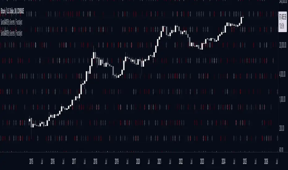
Santa's Secrets | Fractalyst Santa’s Secrets is a visually engaging trading tool that infuses holiday cheer into your charts. Inspired by the enchanting, mysterious vibes of the holiday season, this indicator overlays price charts with dynamic, multi-colored glitches that sync with market data, delivering a festive and whimsical visual experience. The indicator brings a magical touch to your charts, featuring characters from classic holiday themes (e.g., Santa, reindeer, snowflakes, gift boxes) to create a fun and festive “glitch effect.” Users can select a theme for their matrix characters, adding a holiday twist to their trading visuals. As the market data moves, these themed characters are randomly picked and displayed on the chart in a colorful cascade. Underlying Calculations and Logic 1.Character Management: The indicator uses arrays to manage different sets of holiday-themed characters, such as Santa’s sleigh, snowflakes, and reindeer. These arrays allow dynamic selection and update of characters as the market moves, mimicking a festive glitch effect. 2. Current and Previous States: Arrays track the current and previous states of characters, ensuring smooth transitions between visual updates. This dual-state management enables the effects to look like a magical, continuous movement, just like Santa’s sleigh cruising through the winter night. 3. Transparency Control: Transparency levels are controlled through arrays, adjusting opacity to create subtle fading effects or more intense visual appearances. The result is a festive glow that can fade or intensify depending on the market’s volatility. 4. Rain Effect Simulation: To create the “snowfall” or “glitching lights” effect, the indicator manages arrays that simulate falling characters, like snowflakes or candy canes, continuously updating their position and visibility. As new characters enter the top of the screen, older ones disappear from the bottom, with fading transparency to simulate a seamless flow. 5. Operational Flow: • Initialization: Arrays initialize the characters and transparency controls, readying the script for smooth and continuous updates during trading. • Updates: During each cycle, new characters are selected and the old ones shift, with updates in both content and appearance ensuring the matrix effect is visually appealing. • Rendering: The arrays control how the characters are rendered, ensuring the magical holiday effect stays lively and eye-catching without interrupting the trading flow. How to Use Santa’s Secrets Indicator 1. Apply the Indicator to Your Charts: Add the Santa’s Secrets indicator to your chart, activating the holiday-themed visual effect on your selected trading instrument or time frame. 2. Select Your Holiday Theme: In the settings, choose the holiday theme or character set. Whether it’s Santa’s sleigh, reindeer, snowflakes, or gift boxes, pick the one that brings the most festive cheer to your charts. 3. Choose Your Visual Effect (Snowfall or Glitch Burst): Select between the “Snowfall” effect, where characters gently drift down the chart like snowflakes, or the “Glitch Burst” effect, where characters explode outward in a burst of holiday cheer, representing bursts of market volatility. 4. Adjust the Color for Holiday Vibes: Customize the color of the characters to match your chart’s aesthetic or reflect different market conditions. Choose from red for a downtrend, green for an uptrend, or opt for a gradient of colors to capture a true holiday spirit. 5. Fit the Matrix to Your Display: Adjust the width and height of the matrix display to make sure it fits perfectly with your chart layout. Ensure it doesn’t obscure your view while still providing the holiday-themed magic. What Makes Santa’s Secrets Indicator Unique? Holiday Theme Selection: Santa’s Secrets allows traders to choose from a variety of holiday-themed characters. Whether you prefer the traditional Santa’s sleigh, snowflakes, reindeer, or gift boxes, you can bring the festive spirit into your trading. This personalized touch adds a fun, holiday twist to your charts and keeps you engaged during the festive season. Dynamic Effects: Choose between two exciting visual modes – Snowfall Mode or Glitch Burst Mode. The Snowfall Mode brings a gentle, peaceful effect with characters cascading down the chart like snowflakes, while Glitch Burst Mode creates a more intense effect, radiating characters outward in an explosive, holiday-themed display. Customizable Holiday Colors: Traders can fully customize the color of the matrix characters to match their trading environment. Whether you want a traditional red and green for a Christmas mood or a blue and white snow effect, Santa’s Secrets allows you to create the perfect holiday atmosphere while you trade. Universal Display Compatibility: No matter what screen or device you’re using – whether it’s a large monitor, laptop, or mobile – Santa’s Secrets is fully adjustable to fit your screen size. The holiday effect remains visually striking without compromising the integrity of your chart data. Wishing you a happy year filled with success, growth, and profitable trades.🎅🎁 Let's kick off the new year strong with Santa's Secrets! 🚀🎄

Bitcoin Logarithmic Growth Curve 2024 The Bitcoin logarithmic growth curve is a concept used to analyze Bitcoin's price movements over time. The idea is based on the observation that Bitcoin's price tends to grow exponentially, particularly during bull markets. It attempts to give a long-term perspective on the Bitcoin price movements. The curve includes an upper and lower band. These bands often represent zones where Bitcoin's price is overextended (upper band) or undervalued (lower band) relative to its historical growth trajectory. When the price touches or exceeds the upper band, it may indicate a speculative bubble, while prices near the lower band may suggest a buying opportunity. Unlike most Bitcoin growth curve indicators, this one includes a logarithmic growth curve optimized using the latest 2024 price data, making it, in our view, superior to previous models. Additionally, it features statistical confidence intervals derived from linear regression, compatible across all timeframes, and extrapolates the data far into the future. Finally, this model allows users the flexibility to manually adjust the function parameters to suit their preferences. The Bitcoin logarithmic growth curve has the following function: y = 10^(a * log10(x) - b) In the context of this formula, the y value represents the Bitcoin price, while the x value corresponds to the time, specifically indicated by the weekly bar number on the chart. How is it made (You can skip this section if you’re not a fan of math): To optimize the fit of this function and determine the optimal values of a and b, the previous weekly cycle peak values were analyzed. The corresponding x and y values were recorded as follows: 113, 18.55 240, 1004.42 451, 19128.27 655, 65502.47 The same process was applied to the bear market low values: 103, 2.48 267, 211.03 471, 3192.87 676, 16255.15 Next, these values were converted to their linear form by applying the base-10 logarithm. This transformation allows the function to be expressed in a linear state: y = a * x − b. This step is essential for enabling linear regression on these values. For the cycle peak (x,y) values: 2.053, 1.268 2.380, 3.002 2.654, 4.282 2.816, 4.816 And for the bear market low (x,y) values: 2.013, 0.394 2.427, 2.324 2.673, 3.504 2.830, 4.211 Next, linear regression was performed on both these datasets. (Numerous tools are available online for linear regression calculations, making manual computations unnecessary). Linear regression is a method used to find a straight line that best represents the relationship between two variables. It looks at how changes in one variable affect another and tries to predict values based on that relationship. The goal is to minimize the differences between the actual data points and the points predicted by the line. Essentially, it aims to optimize for the highest R-Square value. Below are the results: It is important to note that both the slope (a-value) and the y-intercept (b-value) have associated standard errors. These standard errors can be used to calculate confidence intervals by multiplying them by the t-values (two degrees of freedom) from the linear regression. These t-values can be found in a t-distribution table. For the top cycle confidence intervals, we used t10% (0.133), t25% (0.323), and t33% (0.414). For the bottom cycle confidence intervals, the t-values used were t10% (0.133), t25% (0.323), t33% (0.414), t50% (0.765), and t67% (1.063). The final bull cycle function is: y = 10^(4.058 ± 0.133 * log10(x) – 6.44 ± 0.324) The final bear cycle function is: y = 10^(4.684 ± 0.025 * log10(x) – -9.034 ± 0.063) The main Criticisms of growth curve models: The Bitcoin logarithmic growth curve model faces several general criticisms that we’d like to highlight briefly. The most significant, in our view, is its heavy reliance on past price data, which may not accurately forecast future trends. For instance, previous growth curve models from 2020 on TradingView were overly optimistic in predicting the last cycle’s peak. This is why we aimed to present our process for deriving the final functions in a transparent, step-by-step scientific manner, including statistical confidence intervals. It's important to note that the bull cycle function is less reliable than the bear cycle function, as the top band is significantly wider than the bottom band. Even so, we still believe that the Bitcoin logarithmic growth curve presented in this script is overly optimistic since it goes parly against the concept of diminishing returns which we discussed in this post: This is why we also propose alternative parameter settings that align more closely with the theory of diminishing returns. Our recommendations: Drawing on the concept of diminishing returns, we propose alternative settings for this model that we believe provide a more realistic forecast aligned with this theory. The adjusted parameters apply only to the top band: a-value: 3.637 ± 0.2343 and b-parameter: -5.369 ± 0.6264. However, please note that these values are highly subjective, and you should be aware of the model's limitations. Conservative bull cycle model: y = 10^(3.637 ± 0.2343 * log10(x) - 5.369 ± 0.6264)

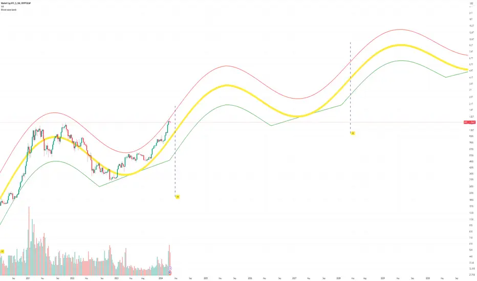
Bitcoin Market Cap wave model weekly This Bitcoin Market Cap wave model indicator is rooted in the foundation of my previously developed tool, the : Bitcoin wave model To derive the Total Market Cap from the Bitcoin wave price model, I employed a straightforward estimation for the Total Market Supply (TMS). This estimation relies on the formula: TMS <= (1 - 2^(-h)) for any h.This equation holds true for any value of h, which will be elaborated upon shortly. It is important to note that this inequality becomes the equality at the dates of halvings, diverging only slightly during other periods. Bitcoin wave model is based on the logarithmic regression model and the sinusoidal waves, induced by the halving events. This chart presents the outcome of an in-depth analysis of the complete set of Bitcoin price data available from October 2009 to August 2023. The central concept is that the logarithm of the Bitcoin price closely adheres to the logarithmic regression model. If we plot the logarithm of the price against the logarithm of time, it forms a nearly straight line. The parameters of this model are provided in the script as follows: log(BTCUSD) = 1.48 + 5.44log(h). The secondary concept involves employing the inherent time unit of Bitcoin instead of days: 'h' denotes a slightly adjusted time measurement intrinsic to the Bitcoin blockchain. It can be approximated as (days since the genesis block) * 0.0007. Precisely, 'h' is defined as follows: h = 0 at the genesis block, h = 1 at the first halving block, and so forth. In general, h = block height / 210,000. Adjustments are made to account for variations in block creation time. The third concept revolves around investigating halving waves triggered by supply shock events resulting from the halvings. These halvings occur at regular intervals in Bitcoin's native time 'h'. All halvings transpire when 'h' is an integer. These events induce waves with intervals denoted as h = 1. Consequently, we can model these waves using a sin(2pih - a) function. The parameter determining the time shift is assessed as 'a = 0.4', aligning with earlier expectations for halving events and their subsequent outcomes. The fourth concept introduces the notion that the waves gradually diminish in amplitude over the progression of "time h," diminishing at a rate of 0.7^h. Lastly, we can create bands around the modeled sinusoidal waves. The upper band is derived by multiplying the sine wave by a factor of 3.1*(1-0.16)^h, while the lower band is obtained by dividing the sine wave by the same factor, 3.1*(1-0.16)^h. The current bandwidth is 2.5x. That means that the upper band is 2.5 times the lower band. These bands are forming an exceptionally narrow predictive channel for Bitcoin. Consequently, a highly accurate estimation of the peak of the next cycle can be derived. The prediction indicates that the zenith past the fourth halving, expected around the summer of 2025, could result in Total Bitcoin Market Cap ranging between 4B and 5B USD. The projections to the future works well only for weekly timeframe. Enjoy the mathematical insights!

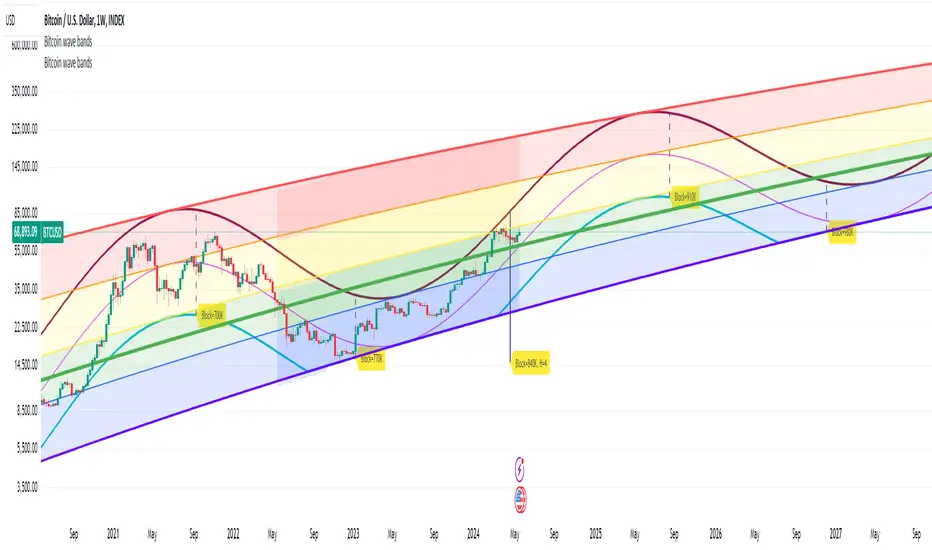
Bitcoin wave model Bitcoin wave model is based on the logarithmic regression model and the sinusoidal waves, induced by the halving events. This chart presents the outcome of an in-depth analysis of the complete set of Bitcoin price data available from October 2009 to August 2023. The central concept is that the logarithm of the Bitcoin price closely adheres to the logarithmic regression model. If we plot the logarithm of the price against the logarithm of time, it forms a nearly straight line. The parameters of this model are provided in the script as follows: log (BTCUSD) = 1.48 + 5.44log(h). The secondary concept involves employing the inherent time unit of Bitcoin instead of days: 'h' denotes a slightly adjusted time measurement intrinsic to the Bitcoin blockchain. It can be approximated as (days since the genesis block) * 0.0007. Precisely, 'h' is defined as follows: h = 0 at the genesis block, h = 1 at the first halving block, and so forth. In general, h = block height / 210,000. Adjustments are made to account for variations in block creation time. The third concept revolves around investigating halving waves triggered by supply shock events resulting from the halvings. These halvings occur at regular intervals in Bitcoin's native time 'h'. All halvings transpire when 'h' is an integer. These events induce waves with intervals denoted as h = 1. Consequently, we can model these waves using a sin(2pih - a) function. The parameter determining the time shift is assessed as 'a = 0.4', aligning with earlier expectations for halving events and their subsequent outcomes. The fourth concept introduces the notion that the waves gradually diminish in amplitude over the progression of "time h," diminishing at a rate of 0.7^h. Lastly, we can create bands around the modeled sinusoidal waves. The upper band is derived by multiplying the sine wave by a factor of 3.1*(1-0.16)^h, while the lower band is obtained by dividing the sine wave by the same factor, 3.1*(1-0.16)^h. The current bandwidth is 2.5x. That means that the upper band is 2.5 times the lower band. These bands are forming an exceptionally narrow predictive channel for Bitcoin. Consequently, a highly accurate estimation of the peak of the next cycle can be derived. The prediction indicates that the zenith past the fourth halving, expected around the summer of 2025, could result in prices ranging between 200,000 and 240,000 USD. Enjoy the mathematical insights!