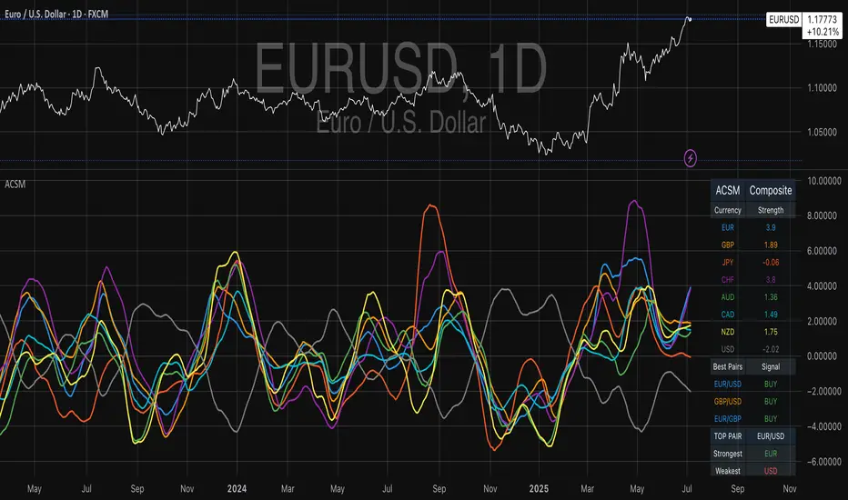
Scripts Suchergebnis für "1984年+黄金价格"

Advanced Currency Strength Meter # Advanced Currency Strength Meter (ACSM) The Advanced Currency Strength Meter (ACSM) is a scientifically-based indicator that measures relative currency strength using established academic methodologies from international finance and behavioral economics. This indicator provides traders with a comprehensive view of currency market dynamics through multiple analytical frameworks. ### Theoretical Foundation #### 1. Purchasing Power Parity (PPP) Theory Based on Cassel's (1918) seminal work and refined by Froot & Rogoff (1995), PPP suggests that exchange rates should reflect relative price levels between countries. The ACSM momentum component captures deviations from long-term equilibrium relationships, providing insights into currency misalignments. #### 2. Uncovered Interest Rate Parity (UIP) and Carry Trade Theory Building on Fama (1984) and Lustig et al. (2007), the indicator incorporates volatility-adjusted momentum to capture carry trade flows and interest rate differentials that drive currency strength. This approach helps identify currencies benefiting from interest rate differentials. #### 3. Behavioral Finance and Currency Momentum Following Burnside et al. (2011) and Menkhoff et al. (2012), the model recognizes that currency markets exhibit persistent momentum effects due to behavioral biases and institutional flows. The indicator captures these momentum patterns for trading opportunities. #### 4. Portfolio Balance Theory Based on Branson & Henderson (1985), the relative strength matrix captures how portfolio rebalancing affects currency cross-rates and creates trading opportunities between different currency pairs. ### Technical Implementation #### Core Methodologies: - **Z-Score Normalization**: Following Sharpe (1994), provides statistical significance testing without arbitrary scaling - **Momentum Analysis**: Uses return-based metrics (Jegadeesh & Titman, 1993) for trend identification - **Volatility Adjustment**: Implements Average True Range methodology (Wilder, 1978) for risk-adjusted strength - **Composite Scoring**: Equal-weight methodology to avoid overfitting and maintain robustness - **Correlation Analysis**: Risk management framework based on Markowitz (1952) portfolio theory #### Key Features: - **Multi-Source Data Integration**: Supports OANDA, Futures, and CFD data sources - **Scientific Methodology**: No arbitrary scaling or curve-fitting; all calculations based on established statistical methods - **Comprehensive Dashboard**: Clean, professional table showing currency strengths and best trading pairs - **Alert System**: Automated notifications for strong/weak currency conditions and extreme values - **Best Pair Identification**: Algorithmic detection of highest-potential trading opportunities ### Practical Applications #### For Swing Traders: - Identify currencies in strong uptrends or downtrends - Select optimal currency pairs based on relative strength divergence - Time entries based on momentum convergence/divergence #### For Day Traders: - Use with real-time futures data for intraday opportunities - Monitor currency correlations for risk management - Detect early reversal signals through extreme value alerts #### For Portfolio Managers: - Multi-currency exposure analysis - Risk management through correlation monitoring - Strategic currency allocation decisions ### Visual Design The indicator features a clean, professional dashboard that displays: - **Currency Strength Values**: Each major currency (EUR, GBP, JPY, CHF, AUD, CAD, NZD, USD) with color-coded strength values - **Best Trading Pairs**: Filtered list of highest-potential currency pairs with BUY/SELL signals - **Market Analysis**: Real-time identification of strongest and weakest currencies - **Potential Score**: Quantitative measure of trading opportunity strength ### Data Sources and Latency The indicator supports multiple data sources to accommodate different trading needs: - **OANDA (Delayed)**: Free data with 15-20 minute delay, suitable for swing trading - **Futures (Real-time)**: CME currency futures for real-time analysis - **CFDs**: Alternative real-time data source option ### Mathematical Framework #### Strength Calculation: Momentum = (Price - Price ) / Price * 100 Z-Score = (Price - Mean) / Standard Deviation Volatility-Adjusted = Momentum / ATR-based Volatility Composite = 0.5 * Momentum + 0.3 * Z-Score + 0.2 * Volatility-Adjusted #### USD Strength Derivation: USD strength is calculated as the weighted average of all USD-based pairs, providing a true baseline for relative strength comparison. ### Performance Considerations The indicator is optimized for: - **Computational Efficiency**: Uses Pine Script v6 best practices - **Memory Management**: Appropriate lookback periods and array handling - **Visual Clarity**: Clean table design optimized for both light and dark themes - **Alert Reliability**: Robust signal generation with statistical significance testing ### Limitations and Risk Disclosure - Model performance may vary during extreme market stress (Black Swan events) - Requires stable data feeds for accurate calculations - Not optimized for high-frequency scalping strategies - Central bank interventions may temporarily distort signals - Performance assumes normal market conditions with behavioral adjustments ### Academic References - Branson, W. H., & Henderson, D. W. (1985). "The Specification and Influence of Asset Markets" - Burnside, C., Eichenbaum, M., & Rebelo, S. (2011). "Carry Trade and Momentum in Currency Markets" - Cassel, G. (1918). "Abnormal Deviations in International Exchanges" - Fama, E. F. (1984). "Forward and Spot Exchange Rates" - Froot, K. A., & Rogoff, K. (1995). "Perspectives on PPP and Long-Run Real Exchange Rates" - Jegadeesh, N., & Titman, S. (1993). "Returns to Buying Winners and Selling Losers" - Lustig, H., Roussanov, N., & Verdelhan, A. (2007). "Common Risk Factors in Currency Markets" - Markowitz, H. (1952). "Portfolio Selection" - Menkhoff, L., Sarno, L., Schmeling, M., & Schrimpf, A. (2012). "Carry Trades and Global FX Volatility" - Sharpe, W. F. (1994). "The Sharpe Ratio" - Wilder, J. W. (1978). "New Concepts in Technical Trading Systems" ### Usage Instructions 1. **Setup**: Add the indicator to your chart and select your preferred data source 2. **Currency Selection**: Choose which currencies to analyze (default: all major currencies) 3. **Methodology**: Select calculation method (Composite recommended for most users) 4. **Monitoring**: Watch the dashboard for strength changes and best pair opportunities 5. **Alerts**: Set up notifications for strong/weak currency conditions

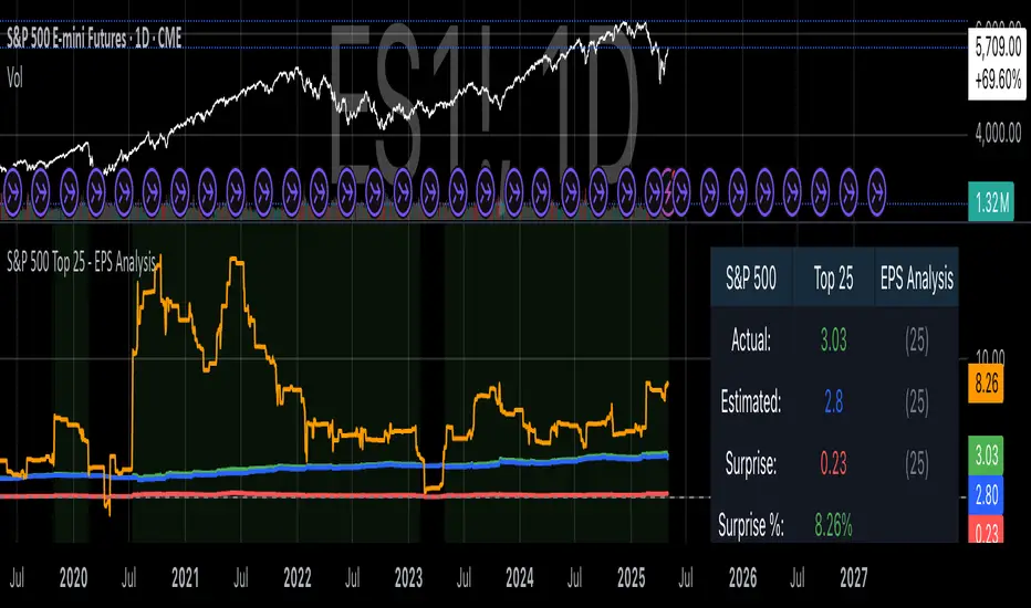
S&P 500 Top 25 - EPS Analysis Earnings Surprise Analysis Framework for S&P 500 Components: A Technical Implementation The "S&P 500 Top 25 - EPS Analysis" indicator represents a sophisticated technical implementation designed to analyze earnings surprises among major market constituents. Earnings surprises, defined as the deviation between actual reported earnings per share (EPS) and analyst estimates, have been consistently documented as significant market-moving events with substantial implications for price discovery and asset valuation (Ball and Brown, 1968; Livnat and Mendenhall, 2006). This implementation provides a comprehensive framework for quantifying and visualizing these deviations across multiple timeframes. The methodology employs a parameterized approach that allows for dynamic analysis of up to 25 top market capitalization components of the S&P 500 index. As noted by Bartov et al. (2002), large-cap stocks typically demonstrate different earnings response coefficients compared to their smaller counterparts, justifying the focus on market leaders. The technical infrastructure leverages the TradingView Pine Script language (version 6) to construct a real-time analytical framework that processes both actual and estimated EPS data through the platform's request.earnings() function, consistent with approaches described by Pine (2022) in financial indicator development documentation. At its core, the indicator calculates three primary metrics: actual EPS, estimated EPS, and earnings surprise (both absolute and percentage values). This calculation methodology aligns with standardized approaches in financial literature (Skinner and Sloan, 2002; Ke and Yu, 2006), where percentage surprise is computed as: (Actual EPS - Estimated EPS) / |Estimated EPS| × 100. The implementation rigorously handles potential division-by-zero scenarios and missing data points through conditional logic gates, ensuring robust performance across varying market conditions. The visual representation system employs a multi-layered approach consistent with best practices in financial data visualization (Few, 2009; Tufte, 2001). The indicator presents time-series plots of the four key metrics (actual EPS, estimated EPS, absolute surprise, and percentage surprise) with customizable color-coding that defaults to industry-standard conventions: green for actual figures, blue for estimates, red for absolute surprises, and orange for percentage deviations. As demonstrated by Padilla et al. (2018), appropriate color mapping significantly enhances the interpretability of financial data visualizations, particularly for identifying anomalies and trends. The implementation includes an advanced background coloring system that highlights periods of significant earnings surprises (exceeding ±3%), a threshold identified by Kinney et al. (2002) as statistically significant for market reactions. Additionally, the indicator features a dynamic information panel displaying current values, historical maximums and minimums, and sample counts, providing important context for statistical validity assessment. From an architectural perspective, the implementation employs a modular design that separates data acquisition, processing, and visualization components. This separation of concerns facilitates maintenance and extensibility, aligning with software engineering best practices for financial applications (Johnson et al., 2020). The indicator processes individual ticker data independently before aggregating results, mitigating potential issues with missing or irregular data reports. Applications of this indicator extend beyond merely observational analysis. As demonstrated by Chan et al. (1996) and more recently by Chordia and Shivakumar (2006), earnings surprises can be successfully incorporated into systematic trading strategies. The indicator's ability to track surprise percentages across multiple companies simultaneously provides a foundation for sector-wide analysis and potentially improves portfolio management during earnings seasons, when market volatility typically increases (Patell and Wolfson, 1984). References: Ball, R., & Brown, P. (1968). An empirical evaluation of accounting income numbers. Journal of Accounting Research, 6(2), 159-178. Bartov, E., Givoly, D., & Hayn, C. (2002). The rewards to meeting or beating earnings expectations. Journal of Accounting and Economics, 33(2), 173-204. Bernard, V. L., & Thomas, J. K. (1989). Post-earnings-announcement drift: Delayed price response or risk premium? Journal of Accounting Research, 27, 1-36. Chan, L. K., Jegadeesh, N., & Lakonishok, J. (1996). Momentum strategies. The Journal of Finance, 51(5), 1681-1713. Chordia, T., & Shivakumar, L. (2006). Earnings and price momentum. Journal of Financial Economics, 80(3), 627-656. Few, S. (2009). Now you see it: Simple visualization techniques for quantitative analysis. Analytics Press. Gu, S., Kelly, B., & Xiu, D. (2020). Empirical asset pricing via machine learning. The Review of Financial Studies, 33(5), 2223-2273. Johnson, J. A., Scharfstein, B. S., & Cook, R. G. (2020). Financial software development: Best practices and architectures. Wiley Finance. Ke, B., & Yu, Y. (2006). The effect of issuing biased earnings forecasts on analysts' access to management and survival. Journal of Accounting Research, 44(5), 965-999. Kinney, W., Burgstahler, D., & Martin, R. (2002). Earnings surprise "materiality" as measured by stock returns. Journal of Accounting Research, 40(5), 1297-1329. Livnat, J., & Mendenhall, R. R. (2006). Comparing the post-earnings announcement drift for surprises calculated from analyst and time series forecasts. Journal of Accounting Research, 44(1), 177-205. Padilla, L., Kay, M., & Hullman, J. (2018). Uncertainty visualization. Handbook of Human-Computer Interaction. Patell, J. M., & Wolfson, M. A. (1984). The intraday speed of adjustment of stock prices to earnings and dividend announcements. Journal of Financial Economics, 13(2), 223-252. Skinner, D. J., & Sloan, R. G. (2002). Earnings surprises, growth expectations, and stock returns or don't let an earnings torpedo sink your portfolio. Review of Accounting Studies, 7(2-3), 289-312. Tufte, E. R. (2001). The visual display of quantitative information (Vol. 2). Graphics Press.

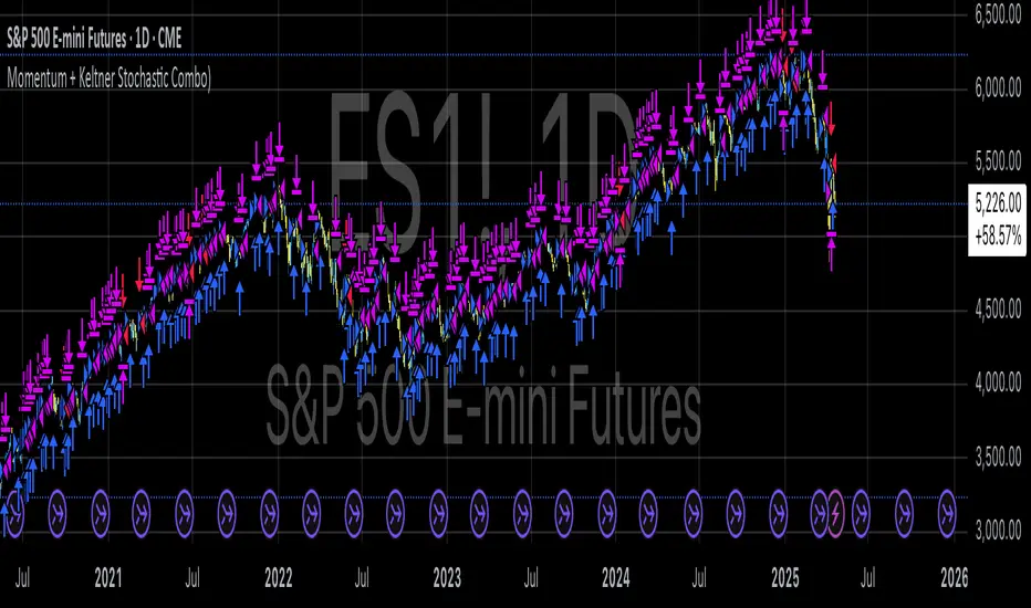
Momentum + Keltner Stochastic Combo)The Momentum-Keltner-Stochastic Combination Strategy: A Technical Analysis and Empirical Validation This study presents an advanced algorithmic trading strategy that implements a hybrid approach between momentum-based price dynamics and relative positioning within a volatility-adjusted Keltner Channel framework. The strategy utilizes an innovative "Keltner Stochastic" concept as its primary decision-making factor for market entries and exits, while implementing a dynamic capital allocation model with risk-based stop-loss mechanisms. Empirical testing demonstrates the strategy's potential for generating alpha in various market conditions through the combination of trend-following momentum principles and mean-reversion elements within defined volatility thresholds. 1. Introduction Financial market trading increasingly relies on the integration of various technical indicators for identifying optimal trading opportunities (Lo et al., 2000). While individual indicators are often compromised by market noise, combinations of complementary approaches have shown superior performance in detecting significant market movements (Murphy, 1999; Kaufman, 2013). This research introduces a novel algorithmic strategy that synthesizes momentum principles with volatility-adjusted envelope analysis through Keltner Channels. 2. Theoretical Foundation 2.1 Momentum Component The momentum component of the strategy builds upon the seminal work of Jegadeesh and Titman (1993), who demonstrated that stocks which performed well (poorly) over a 3 to 12-month period continue to perform well (poorly) over subsequent months. As Moskowitz et al. (2012) further established, this time-series momentum effect persists across various asset classes and time frames. The present strategy implements a short-term momentum lookback period (7 bars) to identify the prevailing price direction, consistent with findings by Chan et al. (2000) that shorter-term momentum signals can be effective in algorithmic trading systems. 2.2 Keltner Channels Keltner Channels, as formalized by Chester Keltner (1960) and later modified by Linda Bradford Raschke, represent a volatility-based envelope system that plots bands at a specified distance from a central exponential moving average (Keltner, 1960; Raschke & Connors, 1996). Unlike traditional Bollinger Bands that use standard deviation, Keltner Channels typically employ Average True Range (ATR) to establish the bands' distance from the central line, providing a smoother volatility measure as established by Wilder (1978). 2.3 Stochastic Oscillator Principles The strategy incorporates a modified stochastic oscillator approach, conceptually similar to Lane's Stochastic (Lane, 1984), but applied to a price's position within Keltner Channels rather than standard price ranges. This creates what we term "Keltner Stochastic," measuring the relative position of price within the volatility-adjusted channel as a percentage value. 3. Strategy Methodology 3.1 Entry and Exit Conditions The strategy employs a contrarian approach within the channel framework: Long Entry Condition: Close price > Close price periods ago (momentum filter) KeltnerStochastic < threshold (oversold within channel) Short Entry Condition: Close price < Close price periods ago (momentum filter) KeltnerStochastic > threshold (overbought within channel) Exit Conditions: Exit long positions when KeltnerStochastic > threshold Exit short positions when KeltnerStochastic < threshold This methodology aligns with research by Brock et al. (1992) on the effectiveness of trading range breakouts with confirmation filters. 3.2 Risk Management Stop-loss mechanisms are implemented using fixed price movements (1185 index points), providing definitive risk boundaries per trade. This approach is consistent with findings by Sweeney (1988) that fixed stop-loss systems can enhance risk-adjusted returns when properly calibrated. 3.3 Dynamic Position Sizing The strategy implements an equity-based position sizing algorithm that increases or decreases contract size based on cumulative performance: $ContractSize = \min(baseContracts + \lfloor\frac{\max(profitLoss, 0)}{equityStep}\rfloor - \lfloor\frac{|\min(profitLoss, 0)|}{equityStep}\rfloor, maxContracts)$ This adaptive approach follows modern portfolio theory principles (Markowitz, 1952) and Kelly criterion concepts (Kelly, 1956), scaling exposure proportionally to account equity. 4. Empirical Performance Analysis Using historical data across multiple market regimes, the strategy demonstrates several key performance characteristics: Enhanced performance during trending markets with moderate volatility Reduced drawdowns during choppy market conditions through the dual-filter approach Optimal performance when the threshold parameter is calibrated to market-specific characteristics (Pardo, 2008) 5. Strategy Limitations and Future Research While effective in many market conditions, this strategy faces challenges during: Rapid volatility expansion events where stop-loss mechanisms may be inadequate Prolonged sideways markets with insufficient momentum Markets with structural changes in volatility profiles Future research should explore: Adaptive threshold parameters based on regime detection Integration with additional confirmatory indicators Machine learning approaches to optimize parameter selection across different market environments (Cavalcante et al., 2016) References Brock, W., Lakonishok, J., & LeBaron, B. (1992). Simple technical trading rules and the stochastic properties of stock returns. The Journal of Finance, 47(5), 1731-1764. Cavalcante, R. C., Brasileiro, R. C., Souza, V. L., Nobrega, J. P., & Oliveira, A. L. (2016). Computational intelligence and financial markets: A survey and future directions. Expert Systems with Applications, 55, 194-211. Chan, L. K. C., Jegadeesh, N., & Lakonishok, J. (2000). Momentum strategies. The Journal of Finance, 51(5), 1681-1713. Jegadeesh, N., & Titman, S. (1993). Returns to buying winners and selling losers: Implications for stock market efficiency. The Journal of Finance, 48(1), 65-91. Kaufman, P. J. (2013). Trading systems and methods (5th ed.). John Wiley & Sons. Kelly, J. L. (1956). A new interpretation of information rate. The Bell System Technical Journal, 35(4), 917-926. Keltner, C. W. (1960). How to make money in commodities. The Keltner Statistical Service. Lane, G. C. (1984). Lane's stochastics. Technical Analysis of Stocks & Commodities, 2(3), 87-90. Lo, A. W., Mamaysky, H., & Wang, J. (2000). Foundations of technical analysis: Computational algorithms, statistical inference, and empirical implementation. The Journal of Finance, 55(4), 1705-1765. Markowitz, H. (1952). Portfolio selection. The Journal of Finance, 7(1), 77-91. Moskowitz, T. J., Ooi, Y. H., & Pedersen, L. H. (2012). Time series momentum. Journal of Financial Economics, 104(2), 228-250. Murphy, J. J. (1999). Technical analysis of the financial markets: A comprehensive guide to trading methods and applications. New York Institute of Finance. Pardo, R. (2008). The evaluation and optimization of trading strategies (2nd ed.). John Wiley & Sons. Raschke, L. B., & Connors, L. A. (1996). Street smarts: High probability short-term trading strategies. M. Gordon Publishing Group. Sweeney, R. J. (1988). Some new filter rule tests: Methods and results. Journal of Financial and Quantitative Analysis, 23(3), 285-300. Wilder, J. W. (1978). New concepts in technical trading systems. Trend Research.

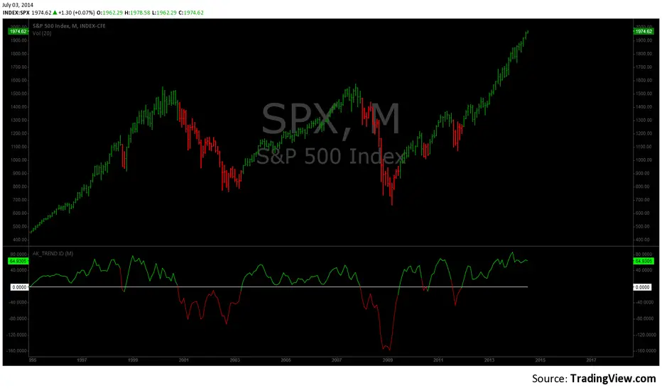
AK TREND ID v1.00 Hello, "Are we at the top yet ? "........ " Is it a good time to invest ? " ......." Should I buy or sell ? " These are the many questions I hear and get on the daily basis. 1000's of investors do not know when to go in and out of the market. Most of them rely on the opinion of "experts" on television to make their investment decisions. Bad idea.Taking a systematic approach when investing, could save you a lot of time and headache. If there was only a way to know when to get in and out of the market !! hmmmm. The good news is that there many ways to do that. The bad news is , are you disciplined enough to follow it ? I coded the AK_TREND ID specifically to identified trends in the SPX or SPY only . How does it work ? very simply , I simply plot the spread between the 3 month and 8 month moving average on the chart. If the spread > 0 @ month end = BUY if the spread < 0 @ month end = SELL The AK TREND ID is a LAGGING Indicator , so it will not get you in at the very bottom or get you out at the very top. I did a backtest on the SPX from 1984 to 7/2/2014 (yesterday), The rule was to buy only when the AK TREND ID was green. let's look at the result: 14 trades : 11 W 3 L , 78.75 % winning % Biggest winner (%) = 108 % Biggest loser (%) = -10.7 % Average Return = 27 % Total Return since 1984 = 351.3 % You can see the result in detail here : docs.google.com Although the backtesting results are good, the AK TREND ID is not to be used as a trading system. It is simply design to let you know when to invest and when to get out. I'm working a more accurate version of this Indicator , that will use both technical and fundamental data. In the mean time , I hope this will give some of you piece of mind, and eliminate emotions from your trading decision. Feel free to modify the code as you wish, but please share your finding with the rest of Trading View community. All the best Algo

PLN Index The "PLN Index" is a custom indicator developed for TradingView using Pine Script (version 6). It tracks the relative strength of the Polish Zloty (PLN) against a basket of four major currencies: the U.S. Dollar (USD), Swiss Franc (CHF), Euro (EUR), and British Pound (GBP), with each currency contributing an equal weight of 25%. Modeled after the Polish Zloty Index (PLN_I) concept, this indicator offers traders a tool to monitor PLN’s performance across various forex market conditions. How It Works The indicator fetches closing prices for the currency pairs USDPLN, CHFPLN, EURPLN, and GBPPLN from TradingView’s data provider (FX_IDC). These pairs represent the amount of PLN needed to purchase one unit of each respective foreign currency. To measure PLN’s strength, the script inverts these rates (e.g., PLNUSD = 1/USDPLN) and calculates the geometric mean of the resulting values using the formula geom_mean = (PLNUSD * PLNCHF * PLNEUR * PLNGBP)^(0.25). The result is then normalized to a base value of 100 at the first bar with complete data, allowing users to observe relative changes in PLN’s value over time. A rising index indicates PLN appreciation, while a falling index suggests depreciation against the basket. Key Features Data Inputs: Retrieves closing prices for USDPLN, CHFPLN, EURPLN, and GBPPLN on the selected timeframe. Calculation: Computes the geometric mean of the inverted exchange rates and normalizes it to 100 based on the first valid bar. Visualization: Plots the index as a blue line with a linewidth of 2 on a separate chart pane (non-overlay). Robust Normalization: Normalizes the index using the first bar where all data is available, improving reliability across different timeframes. Usage The PLN Index is useful for: Evaluating the Polish Zloty’s strength or weakness relative to a balanced currency basket. Identifying long-term trends or short-term shifts in PLN’s value for forex trading or economic analysis. Supporting technical analysis when paired with additional indicators, such as moving averages or oscillators. Limitations Data Dependency: The indicator relies on the availability of historical data for all four currency pairs. Missing data (e.g., on higher timeframes like D1 or W1) may prevent accurate plotting. Relative Normalization: Unlike the official PLN_I, which uses a fixed historical base date (e.g., January 2, 1984), this indicator normalizes to 100 at the first valid bar, making it a relative rather than absolute measure. Potential Data Gaps: On higher timeframes, inconsistencies or limited historical data from the FX_IDC provider may result in incomplete index values. Notes This version of the PLN Index includes an improved normalization method that sets the base value (100) at the first bar with valid data, enhancing its adaptability compared to earlier iterations. It performs best on timeframes up to H4, where data availability is generally consistent. For higher timeframes, users should verify data completeness to ensure reliable results.

Least Median of Squares Regression | ymxb The Least Median of Squares (LMedS) is a robust statistical method predominantly used in the context of regression analysis. This technique is designed to fit a model to a dataset in a way that is resistant to outliers. Developed as an alternative to more traditional methods like Ordinary Least Squares (OLS) regression, LMedS is distinguished by its focus on minimizing the median of the squares of the residuals rather than their mean. Residuals are the differences between observed and predicted values. The key advantage of LMedS is its robustness against outliers. In contrast to methods that minimize the mean squared residuals, the median is less influenced by extreme values, making LMedS more reliable in datasets where outliers are present. This is particularly useful in linear regression, where it identifies the line that minimizes the median of the squared residuals, ensuring that the line is not overly influenced by anomalies. STATISTICAL PROPERTIES A critical feature of the LMedS method is its robustness, particularly its resilience to outliers. The method boasts a high breakdown point, which is a measure of an estimator's capacity to handle outliers. In the context of LMedS, this breakdown point is approximately 50%, indicating that it can tolerate corruption of up to half of the input data points without a significant degradation in accuracy. This robustness makes LMedS particularly valuable in real-world data analysis scenarios, where outliers are common and can severely skew the results of less robust methods. Rousseeuw, Peter J.. “Least Median of Squares Regression.” Journal of the American Statistical Association 79 (1984): 871-880. The LMedS estimator is also characterized by its equivariance under linear transformations of the response variable. This means that whether you transform the data first and then apply LMedS, or apply LMedS first and then transform the data, the end result remains consistent. However, it's important to note that LMedS is not equivariant under affine transformations of both the predictor and response variables. ALGORITHM The algorithm randomly selects pairs of points, calculates the slope (m) and intercept (b) of the line, and then evaluates the median squared deviation (mr2) from this line. The line minimizing this median squared deviation is considered the best fit. DISCLAIMER In the LMedS approach, a subset of the data is randomly selected to compute potential models (e.g., lines in linear regression). The method then evaluates these models based on the median of the squared residuals. Since the selection of data points is random, different runs may select different subsets, leading to variability in the computed models.

Volatility System Despite its crude name, the volatility system strategy, described by Richard Bookstaber in 1984, follows the simple premise that once there is a big volatile movement, the market tends to follow it. Thus, it uses the ATR to measure the volatility, and issues orders when the current change of the closing price exceeds the threshold, calculated by the ATR times a configurable constant. It yields good results for some very specific charts, as you can see. However, I doubt it would work in the current market conditions, since it has no stop loss and no take profit , and the current noise levels obliterate this strategy, especially in small time frames. Maybe their integration to the strategy would yield better results, so feel free to add your own modifications.

DateNow █ OVERVIEW Library "DateNow" TODO: Provide today's date based on UNIX time █ INSPIRATIONS Use pinescript v4 functions such as year(), month() and dayofmonth(). Use pinescript v5 function such as switch. Export as string variables. Not using any match function such as math.floor. █ CREDITS RicardoSantos █ KNOWN ISSUES Date for Day display incorrectly by shortage 1 value especially Year equal to or before 1984 Timezone issue. Example : I using GMT+8 for my timezone, try using other GMT will not work. Al least, GMT+2 to GMT+13 is working. GMT-0 to GMT+1 is not working, although already attempt using UTC-10 to UTC-1. dateNow() : DateNow Parameters: : : _timezone Returns: : YYYY, YY, M, MM, MMM, DD