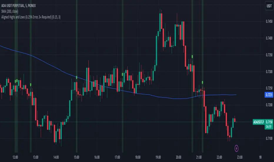
Aligned Highs and Lows (0.25% Error, 3+ Required)This indicator shows when three or more bars in a row have the same end as the previous start within a 0.25% range. This helps identify when there is a possible accumulation or an attempt to break a support or resistance level from an order block.
In den Scripts nach "央行:下调个人住房公积金贷款利率0.25个百分点" suchen
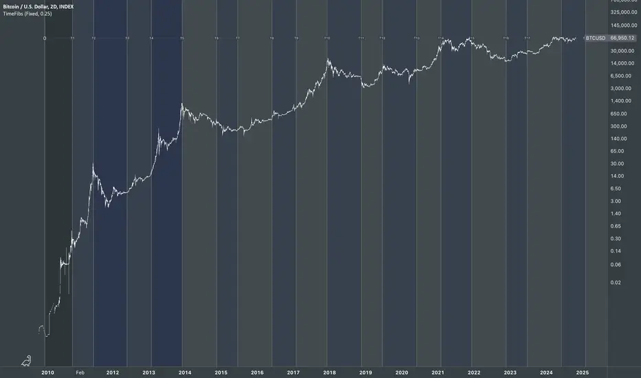
Fibonacci Time PeriodsThe " Fibonacci Time Periods " indicator uses power exponents of the constant Phi based on your custom time period to generate Fibonacci sequence-based progression on a given chart. This tool can help to anticipate the timing of potential turning points by highlighting Fib time zones where significant price movements may occur.
It is different from other alternatives specifically for the ability to alter the rate of progression .
Most famous regular Fib sequence expands with 1.618^(n+1) rate which produces vast change just after few iterations.
Those ever-expanding big intervals don't allow us to cover the smaller details of the chart which we might find crucial. So, the idea was born to break down the constant Phi to a self-fraction using power exponents. In other words, reducing rate of progression to make the expansion more gradual without losing properties of Fibonacci proportions.
Default settings have a rate of 0.25 which is basically Phi^1/4
That means we expect 4x more lines than in regular sequence to cover missing bits owing to formula: 1.618^(0.25*(n+1))
(Line 0.618 is added to enhance visual orientation and perception of proportions)
How it works:
Exponential rate of progression
First, it works out the difference between your custom start (0) and end (1) period
The result is multiplied by 1.618^rate to get the step
Rest lines are created by iterations. For instance, with default rate of 0.25, the 1st generated line = start + (End-Start)*1.618^0.25* 1 , second line = start + (End-Start)*1.618^0.25* 2 , etc.
If we change the rate to 1 it will produce the regular fib sequence with 1.618^(n+1) rate
Fixed rate of progression:
In this mode, when rate is 0.25, it grows exactly with exponent step of 0.25 so first, second, third, etc generated lines also have the fixed exponent of 0.25. The distance between lines do not expand.
How to use:
Set the start and end dates
Choose the type of progression
Choose your desired rate of progression
Customize the colors to match your chart preferences.
Observe the generated Fibonacci time intervals and use them to identify potential market movements and reactions.
2 MA Cross Cvg Dvg Slope Overview
This indicator combines the Moving Average Convergence Divergence (MACD) and two Moving Averages (MAs) to assess market momentum and trend direction. It aims to provide insights into the strength and direction of price movements by analyzing the MACD line, MAs slopes, and MA crossovers. Instead of eyeballing the exact MA crossovers and MAs slope steepness on the chart and MACD line changes on separate panes, this indicator pixelate the overloaded information or multiple indicators interpretation into a KISS "boolean" decision making.
Key Components
MACD Line
This line represents the difference between the fast MA and slow MA. It reflects short-term price momentum relative to the long-term trend.
Moving Averages (MAs)
Two types of MAs are utilized in this indicator:
Fast MA (short-term): Often a 9-period MA or similar, which reacts quickly to price changes.
Slow MA (long-term): Typically a 21-period MA or similar, which smooths out price fluctuations and identifies the longer-term trend.
Indicator Logic
MA Crossover: The crossover of the fast MA above the slow MA suggests a bullish trend, while a crossover below indicates a bearish trend.
MA Slope Analysis: The indicator also considers the slopes of both the fast and slow MAs to determine the direction:
Both MA Positive Slope: Indicates upward momentum or bullish trend.
Both MA Negative Slope: Indicates downward momentum or bearish trend.
One MA Positive Slope, the other Negative Slope: Indicates indecision.
MACD Line: MACD Line consecutively increase means increasing positive momentum, vice versa.
Interpretation
Uptrend: When fast MA cross over slow MA. Indicator show "+" symbol at top zone with value 0.5.
Additional Uptrend Confirmation: When both MAs have positive slope. Indicator show only green bar.
Uptrend Upward Momentum: MACD Line increase when fast MA above slow MA. Indicator show "." symbol value 0.75.
Uptrend Downward Momentum: MACD Line decrease when fast MA above slow MA. Indicator show "." symbol value 0.25.
Indecision: When one of the MA has positive slope, but another MA has negative slope. Indicator showing both red and green bar.
Downtrend: When fast MA cross under slow MA. Indicator show "+" symbol at bottom zone with value 0.5.
Additional Downtrend Confirmation: When both MAs have negative slope. Indicator show only red bar.
Downtrend Upward Momentum: MACD Line increase when fast MA below slow MA. Indicator show "." symbol value -0.25.
Uptrend Downward Momentum: MACD Line decrease when fast MA below slow MA. Indicator show "." symbol value -0.75.
Combination of above multiple interpretation can further derive different signal for Trend Starts, Trend Continuous, and Trend Reversals.
Usage
This indicator is valuable for traders seeking to:
Identify entry and exit points based on single or multiple combination of MAs and MACD Line signals.
Confirm trend direction using MAs cross over or cross under spotted easily with the "+" symbol above 0 or below 0.
Double confirm the trend based on two MAs align slope direction.
Understand momentum shifts and potential trend reversals with an easy 4 different dots at -0.75, -0.25, 0.25, and 0.75.
Conclusion
By combining MACD Line analysis with Moving Average slopes and crossovers, this indicator offers a comprehensive approach to assessing market momentum and trend direction. It provides clear signals for traders to make informed decisions on when to enter or exit positions, enhancing overall trading strategy effectiveness without the need of referring to multiple chart or zoom in and out of the price chart to identify the crossover and slope direction.

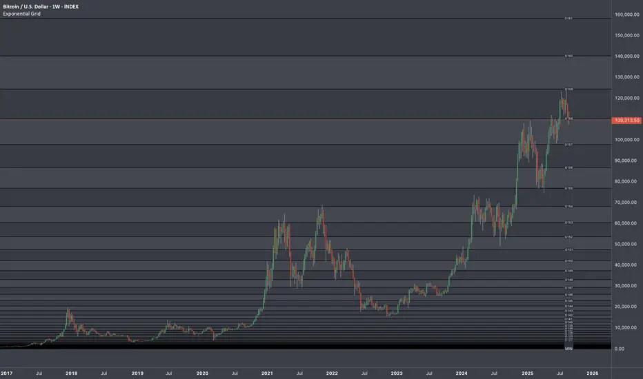
Exponential Grid [Phi, Pi, Euler]If you disagree with one of the EMH principles that price is too random, then by definition you must agree that historic price has deterministic function to a scenario ahead.
I personally believe that constants like phi, pi and e can mimic exponential growth of the price.
In this script, first grid is based on the Lowest price multiplied with self fraction of the constant.
For example:
If you are familiar with fib ratio 1.272, then you must know that it is 1.618 to the power of 0.5.
With default settings of exponent step 0.25
First grid = Lowest price x phi^0.25
Second grid = Lowest price x phi^0.25x2
Third grid = Lowest price x phi^0.25x3 and so on
The script will automatically find the lowest price and update the grid values.
Or you can set up your custom Lowest price manually if you feel like the All Time Low level loses its relevance value after long period.
There are 64 grids including Lowest price level. And it wasn't by a chance. Pine Script has a limitation of max 64 plots. Number of grids shown in the chart depends on the highest price. Once price breaks above ATH a couple of next grids will be plotted automatically. In most cases if everything is plotted, the chart appears squeezed and you'll need to zoom in to see it. Therefore, I adjusted it relatively to the scale of the chart for the comfort.
In some cases 64 plots aren't enough to cover the whole chart. For example, let's take a look at NVIDIA chart:
Since the price has started with 0.0333, it is way too small to cover all with default settings.
We are left with 2 choices:
Either Enable "Round"
OR increase Exponent Step (from 0.25 to 0.5 in the particular example below)
If you set constant to pi or e which is a bigger number than phi, expect the gaps to be bigger. To reduce it to a more gradual way of expansion you can decrease Exponent Step.
Deck@r True Range IndexThis Pine Script calculates the True Range Index (TRI) using ATR and Fib Levels and uses the result to generate buy and sell signals based on certain conditions.
Here's a breakdown of the code:
Inputs:
atr_period: Determines the period for calculating the Average True Range (ATR), preferred setting at 14.
atr_multiplier: Multiplier used to set the width of the ATR bands preferred setting at 1.
Calculations:
atr_value: Calculates the Average True Range (ATR) using the input period.
upper_band: Calculates the upper band of the ATR bands using a Simple Moving Average (SMA) of the close price plus the ATR multiplied by the multiplier.
lower_band: Calculates the lower band of the ATR bands using a Simple Moving Average (SMA) of the close price minus the ATR multiplied by the multiplier.
midline_75 and midline_25: Calculate midlines at Fibonacci retracement levels of 0.75 and 0.25, respectively, between the upper and lower bands.
Plotting:
Plots the upper and lower bands of the ATR bands.
Optionally plots midlines for the ATR bands (commented out in the code).
Buy and Sell Conditions:
buy_condition: Defines a condition for a buy signal, which occurs when the close price is above the midline at the Fibonacci retracement level of 0.25.
sell_condition: Defines a condition for a sell signal, which occurs when the close price is below the midline at the Fibonacci retracement level of 0.75.
Candle Color:
Sets the candle color based on the buy and sell conditions.
Buy and Sell Signals:
buy_signal: Checks for a buy signal when the close price crosses above the midline at the Fibonacci retracement level of 0.25.
sell_signal: Checks for a sell signal when the close price crosses below the midline at the Fibonacci retracement level of 0.75.
Plots buy and sell signals on the chart.

Adaptive Trend Classification: Moving Averages [InvestorUnknown]Adaptive Trend Classification: Moving Averages
Overview
The Adaptive Trend Classification (ATC) Moving Averages indicator is a robust and adaptable investing tool designed to provide dynamic signals based on various types of moving averages and their lengths. This indicator incorporates multiple layers of adaptability to enhance its effectiveness in various market conditions.
Key Features
Adaptability of Moving Average Types and Lengths: The indicator utilizes different types of moving averages (EMA, HMA, WMA, DEMA, LSMA, KAMA) with customizable lengths to adjust to market conditions.
Dynamic Weighting Based on Performance: ] Weights are assigned to each moving average based on the equity they generate, with considerations for a cutout period and decay rate to manage (reduce) the influence of past performances.
Exponential Growth Adjustment: The influence of recent performance is enhanced through an adjustable exponential growth factor, ensuring that more recent data has a greater impact on the signal.
Calibration Mode: Allows users to fine-tune the indicator settings for specific signal periods and backtesting, ensuring optimized performance.
Visualization Options: Multiple customization options for plotting moving averages, color bars, and signal arrows, enhancing the clarity of the visual output.
Alerts: Configurable alert settings to notify users based on specific moving average crossovers or the average signal.
User Inputs
Adaptability Settings
λ (Lambda): Specifies the growth rate for exponential growth calculations.
Decay (%): Determines the rate of depreciation applied to the equity over time.
CutOut Period: Sets the period after which equity calculations start, allowing for a focus on specific time ranges.
Robustness Lengths: Defines the range of robustness for equity calculation with options for Narrow, Medium, or Wide adjustments.
Long/Short Threshold: Sets thresholds for long and short signals.
Calculation Source: The data source used for calculations (e.g., close price).
Moving Averages Settings
Lengths and Weights: Allows customization of lengths and initial weights for each moving average type (EMA, HMA, WMA, DEMA, LSMA, KAMA).
Calibration Mode
Calibration Mode: Enables calibration for fine-tuning inputs.
Calibrate: Specifies which moving average type to calibrate.
Strategy View: Shifts entries and exits by one bar for non-repainting backtesting.
Calculation Logic
Rate of Change (R): Calculates the rate of change in the price.
Set of Moving Averages: Generates multiple moving averages with different lengths for each type.
diflen(length) =>
int L1 = na, int L_1 = na
int L2 = na, int L_2 = na
int L3 = na, int L_3 = na
int L4 = na, int L_4 = na
if robustness == "Narrow"
L1 := length + 1, L_1 := length - 1
L2 := length + 2, L_2 := length - 2
L3 := length + 3, L_3 := length - 3
L4 := length + 4, L_4 := length - 4
else if robustness == "Medium"
L1 := length + 1, L_1 := length - 1
L2 := length + 2, L_2 := length - 2
L3 := length + 4, L_3 := length - 4
L4 := length + 6, L_4 := length - 6
else
L1 := length + 1, L_1 := length - 1
L2 := length + 3, L_2 := length - 3
L3 := length + 5, L_3 := length - 5
L4 := length + 7, L_4 := length - 7
// Function to calculate different types of moving averages
ma_calculation(source, length, ma_type) =>
if ma_type == "EMA"
ta.ema(source, length)
else if ma_type == "HMA"
ta.sma(source, length)
else if ma_type == "WMA"
ta.wma(source, length)
else if ma_type == "DEMA"
ta.dema(source, length)
else if ma_type == "LSMA"
lsma(source,length)
else if ma_type == "KAMA"
kama(source, length)
else
na
// Function to create a set of moving averages with different lengths
SetOfMovingAverages(length, source, ma_type) =>
= diflen(length)
MA = ma_calculation(source, length, ma_type)
MA1 = ma_calculation(source, L1, ma_type)
MA2 = ma_calculation(source, L2, ma_type)
MA3 = ma_calculation(source, L3, ma_type)
MA4 = ma_calculation(source, L4, ma_type)
MA_1 = ma_calculation(source, L_1, ma_type)
MA_2 = ma_calculation(source, L_2, ma_type)
MA_3 = ma_calculation(source, L_3, ma_type)
MA_4 = ma_calculation(source, L_4, ma_type)
Exponential Growth Factor: Computes an exponential growth factor based on the current bar index and growth rate.
// The function `e(L)` calculates an exponential growth factor based on the current bar index and a given growth rate `L`.
e(L) =>
// Calculate the number of bars elapsed.
// If the `bar_index` is 0 (i.e., the very first bar), set `bars` to 1 to avoid division by zero.
bars = bar_index == 0 ? 1 : bar_index
// Define the cuttime time using the `cutout` parameter, which specifies how many bars will be cut out off the time series.
cuttime = time
// Initialize the exponential growth factor `x` to 1.0.
x = 1.0
// Check if `cuttime` is not `na` and the current time is greater than or equal to `cuttime`.
if not na(cuttime) and time >= cuttime
// Use the mathematical constant `e` raised to the power of `L * (bar_index - cutout)`.
// This represents exponential growth over the number of bars since the `cutout`.
x := math.pow(math.e, L * (bar_index - cutout))
x
Equity Calculation: Calculates the equity based on starting equity, signals, and the rate of change, incorporating a natural decay rate.
pine code
// This function calculates the equity based on the starting equity, signals, and rate of change (R).
eq(starting_equity, sig, R) =>
cuttime = time
if not na(cuttime) and time >= cuttime
// Calculate the rate of return `r` by multiplying the rate of change `R` with the exponential growth factor `e(La)`.
r = R * e(La)
// Calculate the depreciation factor `d` as 1 minus the depreciation rate `De`.
d = 1 - De
var float a = 0.0
// If the previous signal `sig ` is positive, set `a` to `r`.
if (sig > 0)
a := r
// If the previous signal `sig ` is negative, set `a` to `-r`.
else if (sig < 0)
a := -r
// Declare the variable `e` to store equity and initialize it to `na`.
var float e = na
// If `e ` (the previous equity value) is not available (first calculation):
if na(e )
e := starting_equity
else
// Update `e` based on the previous equity value, depreciation factor `d`, and adjustment factor `a`.
e := (e * d) * (1 + a)
// Ensure `e` does not drop below 0.25.
if (e < 0.25)
e := 0.25
e
else
na
Signal Generation: Generates signals based on crossovers and computes a weighted signal from multiple moving averages.
Main Calculations
The indicator calculates different moving averages (EMA, HMA, WMA, DEMA, LSMA, KAMA) and their respective signals, applies exponential growth and decay factors to compute equities, and then derives a final signal by averaging weighted signals from all moving averages.
Visualization and Alerts
The final signal, along with additional visual aids like color bars and arrows, is plotted on the chart. Users can also set up alerts based on specific conditions to receive notifications for potential trading opportunities.
Repainting
The indicator does support intra-bar changes of signal but will not repaint once the bar is closed, if you want to get alerts only for signals after bar close, turn on “Strategy View” while setting up the alert.
Conclusion
The Adaptive Trend Classification: Moving Averages Indicator is a sophisticated tool for investors, offering extensive customization and adaptability to changing market conditions. By integrating multiple moving averages and leveraging dynamic weighting based on performance, it aims to provide reliable and timely investing signals.

Tensor Market Analysis Engine (TMAE)# Tensor Market Analysis Engine (TMAE)
## Advanced Multi-Dimensional Mathematical Analysis System
*Where Quantum Mathematics Meets Market Structure*
---
## 🎓 THEORETICAL FOUNDATION
The Tensor Market Analysis Engine represents a revolutionary synthesis of three cutting-edge mathematical frameworks that have never before been combined for comprehensive market analysis. This indicator transcends traditional technical analysis by implementing advanced mathematical concepts from quantum mechanics, information theory, and fractal geometry.
### 🌊 Multi-Dimensional Volatility with Jump Detection
**Hawkes Process Implementation:**
The TMAE employs a sophisticated Hawkes process approximation for detecting self-exciting market jumps. Unlike traditional volatility measures that treat price movements as independent events, the Hawkes process recognizes that market shocks cluster and exhibit memory effects.
**Mathematical Foundation:**
```
Intensity λ(t) = μ + Σ α(t - Tᵢ)
```
Where market jumps at times Tᵢ increase the probability of future jumps through the decay function α, controlled by the Hawkes Decay parameter (0.5-0.99).
**Mahalanobis Distance Calculation:**
The engine calculates volatility jumps using multi-dimensional Mahalanobis distance across up to 5 volatility dimensions:
- **Dimension 1:** Price volatility (standard deviation of returns)
- **Dimension 2:** Volume volatility (normalized volume fluctuations)
- **Dimension 3:** Range volatility (high-low spread variations)
- **Dimension 4:** Correlation volatility (price-volume relationship changes)
- **Dimension 5:** Microstructure volatility (intrabar positioning analysis)
This creates a volatility state vector that captures market behavior impossible to detect with traditional single-dimensional approaches.
### 📐 Hurst Exponent Regime Detection
**Fractal Market Hypothesis Integration:**
The TMAE implements advanced Rescaled Range (R/S) analysis to calculate the Hurst exponent in real-time, providing dynamic regime classification:
- **H > 0.6:** Trending (persistent) markets - momentum strategies optimal
- **H < 0.4:** Mean-reverting (anti-persistent) markets - contrarian strategies optimal
- **H ≈ 0.5:** Random walk markets - breakout strategies preferred
**Adaptive R/S Analysis:**
Unlike static implementations, the TMAE uses adaptive windowing that adjusts to market conditions:
```
H = log(R/S) / log(n)
```
Where R is the range of cumulative deviations and S is the standard deviation over period n.
**Dynamic Regime Classification:**
The system employs hysteresis to prevent regime flipping, requiring sustained Hurst values before regime changes are confirmed. This prevents false signals during transitional periods.
### 🔄 Transfer Entropy Analysis
**Information Flow Quantification:**
Transfer entropy measures the directional flow of information between price and volume, revealing lead-lag relationships that indicate future price movements:
```
TE(X→Y) = Σ p(yₜ₊₁, yₜ, xₜ) log
```
**Causality Detection:**
- **Volume → Price:** Indicates accumulation/distribution phases
- **Price → Volume:** Suggests retail participation or momentum chasing
- **Balanced Flow:** Market equilibrium or transition periods
The system analyzes multiple lag periods (2-20 bars) to capture both immediate and structural information flows.
---
## 🔧 COMPREHENSIVE INPUT SYSTEM
### Core Parameters Group
**Primary Analysis Window (10-100, Default: 50)**
The fundamental lookback period affecting all calculations. Optimization by timeframe:
- **1-5 minute charts:** 20-30 (rapid adaptation to micro-movements)
- **15 minute-1 hour:** 30-50 (balanced responsiveness and stability)
- **4 hour-daily:** 50-100 (smooth signals, reduced noise)
- **Asset-specific:** Cryptocurrency 20-35, Stocks 35-50, Forex 40-60
**Signal Sensitivity (0.1-2.0, Default: 0.7)**
Master control affecting all threshold calculations:
- **Conservative (0.3-0.6):** High-quality signals only, fewer false positives
- **Balanced (0.7-1.0):** Optimal risk-reward ratio for most trading styles
- **Aggressive (1.1-2.0):** Maximum signal frequency, requires careful filtering
**Signal Generation Mode:**
- **Aggressive:** Any component signals (highest frequency)
- **Confluence:** 2+ components agree (balanced approach)
- **Conservative:** All 3 components align (highest quality)
### Volatility Jump Detection Group
**Volatility Dimensions (2-5, Default: 3)**
Determines the mathematical space complexity:
- **2D:** Price + Volume volatility (suitable for clean markets)
- **3D:** + Range volatility (optimal for most conditions)
- **4D:** + Correlation volatility (advanced multi-asset analysis)
- **5D:** + Microstructure volatility (maximum sensitivity)
**Jump Detection Threshold (1.5-4.0σ, Default: 3.0σ)**
Standard deviations required for volatility jump classification:
- **Cryptocurrency:** 2.0-2.5σ (naturally volatile)
- **Stock Indices:** 2.5-3.0σ (moderate volatility)
- **Forex Major Pairs:** 3.0-3.5σ (typically stable)
- **Commodities:** 2.0-3.0σ (varies by commodity)
**Jump Clustering Decay (0.5-0.99, Default: 0.85)**
Hawkes process memory parameter:
- **0.5-0.7:** Fast decay (jumps treated as independent)
- **0.8-0.9:** Moderate clustering (realistic market behavior)
- **0.95-0.99:** Strong clustering (crisis/event-driven markets)
### Hurst Exponent Analysis Group
**Calculation Method Options:**
- **Classic R/S:** Original Rescaled Range (fast, simple)
- **Adaptive R/S:** Dynamic windowing (recommended for trading)
- **DFA:** Detrended Fluctuation Analysis (best for noisy data)
**Trending Threshold (0.55-0.8, Default: 0.60)**
Hurst value defining persistent market behavior:
- **0.55-0.60:** Weak trend persistence
- **0.65-0.70:** Clear trending behavior
- **0.75-0.80:** Strong momentum regimes
**Mean Reversion Threshold (0.2-0.45, Default: 0.40)**
Hurst value defining anti-persistent behavior:
- **0.35-0.45:** Weak mean reversion
- **0.25-0.35:** Clear ranging behavior
- **0.15-0.25:** Strong reversion tendency
### Transfer Entropy Parameters Group
**Information Flow Analysis:**
- **Price-Volume:** Classic flow analysis for accumulation/distribution
- **Price-Volatility:** Risk flow analysis for sentiment shifts
- **Multi-Timeframe:** Cross-timeframe causality detection
**Maximum Lag (2-20, Default: 5)**
Causality detection window:
- **2-5 bars:** Immediate causality (scalping)
- **5-10 bars:** Short-term flow (day trading)
- **10-20 bars:** Structural flow (swing trading)
**Significance Threshold (0.05-0.3, Default: 0.15)**
Minimum entropy for signal generation:
- **0.05-0.10:** Detect subtle information flows
- **0.10-0.20:** Clear causality only
- **0.20-0.30:** Very strong flows only
---
## 🎨 ADVANCED VISUAL SYSTEM
### Tensor Volatility Field Visualization
**Five-Layer Resonance Bands:**
The tensor field creates dynamic support/resistance zones that expand and contract based on mathematical field strength:
- **Core Layer (Purple):** Primary tensor field with highest intensity
- **Layer 2 (Neutral):** Secondary mathematical resonance
- **Layer 3 (Info Blue):** Tertiary harmonic frequencies
- **Layer 4 (Warning Gold):** Outer field boundaries
- **Layer 5 (Success Green):** Maximum field extension
**Field Strength Calculation:**
```
Field Strength = min(3.0, Mahalanobis Distance × Tensor Intensity)
```
The field amplitude adjusts to ATR and mathematical distance, creating dynamic zones that respond to market volatility.
**Radiation Line Network:**
During active tensor states, the system projects directional radiation lines showing field energy distribution:
- **8 Directional Rays:** Complete angular coverage
- **Tapering Segments:** Progressive transparency for natural visual flow
- **Pulse Effects:** Enhanced visualization during volatility jumps
### Dimensional Portal System
**Portal Mathematics:**
Dimensional portals visualize regime transitions using category theory principles:
- **Green Portals (◉):** Trending regime detection (appear below price for support)
- **Red Portals (◎):** Mean-reverting regime (appear above price for resistance)
- **Yellow Portals (○):** Random walk regime (neutral positioning)
**Tensor Trail Effects:**
Each portal generates 8 trailing particles showing mathematical momentum:
- **Large Particles (●):** Strong mathematical signal
- **Medium Particles (◦):** Moderate signal strength
- **Small Particles (·):** Weak signal continuation
- **Micro Particles (˙):** Signal dissipation
### Information Flow Streams
**Particle Stream Visualization:**
Transfer entropy creates flowing particle streams indicating information direction:
- **Upward Streams:** Volume leading price (accumulation phases)
- **Downward Streams:** Price leading volume (distribution phases)
- **Stream Density:** Proportional to information flow strength
**15-Particle Evolution:**
Each stream contains 15 particles with progressive sizing and transparency, creating natural flow visualization that makes information transfer immediately apparent.
### Fractal Matrix Grid System
**Multi-Timeframe Fractal Levels:**
The system calculates and displays fractal highs/lows across five Fibonacci periods:
- **8-Period:** Short-term fractal structure
- **13-Period:** Intermediate-term patterns
- **21-Period:** Primary swing levels
- **34-Period:** Major structural levels
- **55-Period:** Long-term fractal boundaries
**Triple-Layer Visualization:**
Each fractal level uses three-layer rendering:
- **Shadow Layer:** Widest, darkest foundation (width 5)
- **Glow Layer:** Medium white core line (width 3)
- **Tensor Layer:** Dotted mathematical overlay (width 1)
**Intelligent Labeling System:**
Smart spacing prevents label overlap using ATR-based minimum distances. Labels include:
- **Fractal Period:** Time-based identification
- **Topological Class:** Mathematical complexity rating (0, I, II, III)
- **Price Level:** Exact fractal price
- **Mahalanobis Distance:** Current mathematical field strength
- **Hurst Exponent:** Current regime classification
- **Anomaly Indicators:** Visual strength representations (○ ◐ ● ⚡)
### Wick Pressure Analysis
**Rejection Level Mathematics:**
The system analyzes candle wick patterns to project future pressure zones:
- **Upper Wick Analysis:** Identifies selling pressure and resistance zones
- **Lower Wick Analysis:** Identifies buying pressure and support zones
- **Pressure Projection:** Extends lines forward based on mathematical probability
**Multi-Layer Glow Effects:**
Wick pressure lines use progressive transparency (1-8 layers) creating natural glow effects that make pressure zones immediately visible without cluttering the chart.
### Enhanced Regime Background
**Dynamic Intensity Mapping:**
Background colors reflect mathematical regime strength:
- **Deep Transparency (98% alpha):** Subtle regime indication
- **Pulse Intensity:** Based on regime strength calculation
- **Color Coding:** Green (trending), Red (mean-reverting), Neutral (random)
**Smoothing Integration:**
Regime changes incorporate 10-bar smoothing to prevent background flicker while maintaining responsiveness to genuine regime shifts.
### Color Scheme System
**Six Professional Themes:**
- **Dark (Default):** Professional trading environment optimization
- **Light:** High ambient light conditions
- **Classic:** Traditional technical analysis appearance
- **Neon:** High-contrast visibility for active trading
- **Neutral:** Minimal distraction focus
- **Bright:** Maximum visibility for complex setups
Each theme maintains mathematical accuracy while optimizing visual clarity for different trading environments and personal preferences.
---
## 📊 INSTITUTIONAL-GRADE DASHBOARD
### Tensor Field Status Section
**Field Strength Display:**
Real-time Mahalanobis distance calculation with dynamic emoji indicators:
- **⚡ (Lightning):** Extreme field strength (>1.5× threshold)
- **● (Solid Circle):** Strong field activity (>1.0× threshold)
- **○ (Open Circle):** Normal field state
**Signal Quality Rating:**
Democratic algorithm assessment:
- **ELITE:** All 3 components aligned (highest probability)
- **STRONG:** 2 components aligned (good probability)
- **GOOD:** 1 component active (moderate probability)
- **WEAK:** No clear component signals
**Threshold and Anomaly Monitoring:**
- **Threshold Display:** Current mathematical threshold setting
- **Anomaly Level (0-100%):** Combined volatility and volume spike measurement
- **>70%:** High anomaly (red warning)
- **30-70%:** Moderate anomaly (orange caution)
- **<30%:** Normal conditions (green confirmation)
### Tensor State Analysis Section
**Mathematical State Classification:**
- **↑ BULL (Tensor State +1):** Trending regime with bullish bias
- **↓ BEAR (Tensor State -1):** Mean-reverting regime with bearish bias
- **◈ SUPER (Tensor State 0):** Random walk regime (neutral)
**Visual State Gauge:**
Five-circle progression showing tensor field polarity:
- **🟢🟢🟢⚪⚪:** Strong bullish mathematical alignment
- **⚪⚪🟡⚪⚪:** Neutral/transitional state
- **⚪⚪🔴🔴🔴:** Strong bearish mathematical alignment
**Trend Direction and Phase Analysis:**
- **📈 BULL / 📉 BEAR / ➡️ NEUTRAL:** Primary trend classification
- **🌪️ CHAOS:** Extreme information flow (>2.0 flow strength)
- **⚡ ACTIVE:** Strong information flow (1.0-2.0 flow strength)
- **😴 CALM:** Low information flow (<1.0 flow strength)
### Trading Signals Section
**Real-Time Signal Status:**
- **🟢 ACTIVE / ⚪ INACTIVE:** Long signal availability
- **🔴 ACTIVE / ⚪ INACTIVE:** Short signal availability
- **Components (X/3):** Active algorithmic components
- **Mode Display:** Current signal generation mode
**Signal Strength Visualization:**
Color-coded component count:
- **Green:** 3/3 components (maximum confidence)
- **Aqua:** 2/3 components (good confidence)
- **Orange:** 1/3 components (moderate confidence)
- **Gray:** 0/3 components (no signals)
### Performance Metrics Section
**Win Rate Monitoring:**
Estimated win rates based on signal quality with emoji indicators:
- **🔥 (Fire):** ≥60% estimated win rate
- **👍 (Thumbs Up):** 45-59% estimated win rate
- **⚠️ (Warning):** <45% estimated win rate
**Mathematical Metrics:**
- **Hurst Exponent:** Real-time fractal dimension (0.000-1.000)
- **Information Flow:** Volume/price leading indicators
- **📊 VOL:** Volume leading price (accumulation/distribution)
- **💰 PRICE:** Price leading volume (momentum/speculation)
- **➖ NONE:** Balanced information flow
- **Volatility Classification:**
- **🔥 HIGH:** Above 1.5× jump threshold
- **📊 NORM:** Normal volatility range
- **😴 LOW:** Below 0.5× jump threshold
### Market Structure Section (Large Dashboard)
**Regime Classification:**
- **📈 TREND:** Hurst >0.6, momentum strategies optimal
- **🔄 REVERT:** Hurst <0.4, contrarian strategies optimal
- **🎲 RANDOM:** Hurst ≈0.5, breakout strategies preferred
**Mathematical Field Analysis:**
- **Dimensions:** Current volatility space complexity (2D-5D)
- **Hawkes λ (Lambda):** Self-exciting jump intensity (0.00-1.00)
- **Jump Status:** 🚨 JUMP (active) / ✅ NORM (normal)
### Settings Summary Section (Large Dashboard)
**Active Configuration Display:**
- **Sensitivity:** Current master sensitivity setting
- **Lookback:** Primary analysis window
- **Theme:** Active color scheme
- **Method:** Hurst calculation method (Classic R/S, Adaptive R/S, DFA)
**Dashboard Sizing Options:**
- **Small:** Essential metrics only (mobile/small screens)
- **Normal:** Balanced information density (standard desktop)
- **Large:** Maximum detail (multi-monitor setups)
**Position Options:**
- **Top Right:** Standard placement (avoids price action)
- **Top Left:** Wide chart optimization
- **Bottom Right:** Recent price focus (scalping)
- **Bottom Left:** Maximum price visibility (swing trading)
---
## 🎯 SIGNAL GENERATION LOGIC
### Multi-Component Convergence System
**Component Signal Architecture:**
The TMAE generates signals through sophisticated component analysis rather than simple threshold crossing:
**Volatility Component:**
- **Jump Detection:** Mahalanobis distance threshold breach
- **Hawkes Intensity:** Self-exciting process activation (>0.2)
- **Multi-dimensional:** Considers all volatility dimensions simultaneously
**Hurst Regime Component:**
- **Trending Markets:** Price above SMA-20 with positive momentum
- **Mean-Reverting Markets:** Price at Bollinger Band extremes
- **Random Markets:** Bollinger squeeze breakouts with directional confirmation
**Transfer Entropy Component:**
- **Volume Leadership:** Information flow from volume to price
- **Volume Spike:** Volume 110%+ above 20-period average
- **Flow Significance:** Above entropy threshold with directional bias
### Democratic Signal Weighting
**Signal Mode Implementation:**
- **Aggressive Mode:** Any single component triggers signal
- **Confluence Mode:** Minimum 2 components must agree
- **Conservative Mode:** All 3 components must align
**Momentum Confirmation:**
All signals require momentum confirmation:
- **Long Signals:** RSI >50 AND price >EMA-9
- **Short Signals:** RSI <50 AND price 0.6):**
- **Increase Sensitivity:** Catch momentum continuation
- **Lower Mean Reversion Threshold:** Avoid counter-trend signals
- **Emphasize Volume Leadership:** Institutional accumulation/distribution
- **Tensor Field Focus:** Use expansion for trend continuation
- **Signal Mode:** Aggressive or Confluence for trend following
**Range-Bound Markets (Hurst <0.4):**
- **Decrease Sensitivity:** Avoid false breakouts
- **Lower Trending Threshold:** Quick regime recognition
- **Focus on Price Leadership:** Retail sentiment extremes
- **Fractal Grid Emphasis:** Support/resistance trading
- **Signal Mode:** Conservative for high-probability reversals
**Volatile Markets (High Jump Frequency):**
- **Increase Hawkes Decay:** Recognize event clustering
- **Higher Jump Threshold:** Avoid noise signals
- **Maximum Dimensions:** Capture full volatility complexity
- **Reduce Position Sizing:** Risk management adaptation
- **Enhanced Visuals:** Maximum information for rapid decisions
**Low Volatility Markets (Low Jump Frequency):**
- **Decrease Jump Threshold:** Capture subtle movements
- **Lower Hawkes Decay:** Treat moves as independent
- **Reduce Dimensions:** Simplify analysis
- **Increase Position Sizing:** Capitalize on compressed volatility
- **Minimal Visuals:** Reduce distraction in quiet markets
---
## 🚀 ADVANCED TRADING STRATEGIES
### The Mathematical Convergence Method
**Entry Protocol:**
1. **Fractal Grid Approach:** Monitor price approaching significant fractal levels
2. **Tensor Field Confirmation:** Verify field expansion supporting direction
3. **Portal Signal:** Wait for dimensional portal appearance
4. **ELITE/STRONG Quality:** Only trade highest quality mathematical signals
5. **Component Consensus:** Confirm 2+ components agree in Confluence mode
**Example Implementation:**
- Price approaching 21-period fractal high
- Tensor field expanding upward (bullish mathematical alignment)
- Green portal appears below price (trending regime confirmation)
- ELITE quality signal with 3/3 components active
- Enter long position with stop below fractal level
**Risk Management:**
- **Stop Placement:** Below/above fractal level that generated signal
- **Position Sizing:** Based on Mahalanobis distance (higher distance = smaller size)
- **Profit Targets:** Next fractal level or tensor field resistance
### The Regime Transition Strategy
**Regime Change Detection:**
1. **Monitor Hurst Exponent:** Watch for persistent moves above/below thresholds
2. **Portal Color Change:** Regime transitions show different portal colors
3. **Background Intensity:** Increasing regime background intensity
4. **Mathematical Confirmation:** Wait for regime confirmation (hysteresis)
**Trading Implementation:**
- **Trending Transitions:** Trade momentum breakouts, follow trend
- **Mean Reversion Transitions:** Trade range boundaries, fade extremes
- **Random Transitions:** Trade breakouts with tight stops
**Advanced Techniques:**
- **Multi-Timeframe:** Confirm regime on higher timeframe
- **Early Entry:** Enter on regime transition rather than confirmation
- **Regime Strength:** Larger positions during strong regime signals
### The Information Flow Momentum Strategy
**Flow Detection Protocol:**
1. **Monitor Transfer Entropy:** Watch for significant information flow shifts
2. **Volume Leadership:** Strong edge when volume leads price
3. **Flow Acceleration:** Increasing flow strength indicates momentum
4. **Directional Confirmation:** Ensure flow aligns with intended trade direction
**Entry Signals:**
- **Volume → Price Flow:** Enter during accumulation/distribution phases
- **Price → Volume Flow:** Enter on momentum confirmation breaks
- **Flow Reversal:** Counter-trend entries when flow reverses
**Optimization:**
- **Scalping:** Use immediate flow detection (2-5 bar lag)
- **Swing Trading:** Use structural flow (10-20 bar lag)
- **Multi-Asset:** Compare flow between correlated assets
### The Tensor Field Expansion Strategy
**Field Mathematics:**
The tensor field expansion indicates mathematical pressure building in market structure:
**Expansion Phases:**
1. **Compression:** Field contracts, volatility decreases
2. **Tension Building:** Mathematical pressure accumulates
3. **Expansion:** Field expands rapidly with directional movement
4. **Resolution:** Field stabilizes at new equilibrium
**Trading Applications:**
- **Compression Trading:** Prepare for breakout during field contraction
- **Expansion Following:** Trade direction of field expansion
- **Reversion Trading:** Fade extreme field expansion
- **Multi-Dimensional:** Consider all field layers for confirmation
### The Hawkes Process Event Strategy
**Self-Exciting Jump Trading:**
Understanding that market shocks cluster and create follow-on opportunities:
**Jump Sequence Analysis:**
1. **Initial Jump:** First volatility jump detected
2. **Clustering Phase:** Hawkes intensity remains elevated
3. **Follow-On Opportunities:** Additional jumps more likely
4. **Decay Period:** Intensity gradually decreases
**Implementation:**
- **Jump Confirmation:** Wait for mathematical jump confirmation
- **Direction Assessment:** Use other components for direction
- **Clustering Trades:** Trade subsequent moves during high intensity
- **Decay Exit:** Exit positions as Hawkes intensity decays
### The Fractal Confluence System
**Multi-Timeframe Fractal Analysis:**
Combining fractal levels across different periods for high-probability zones:
**Confluence Zones:**
- **Double Confluence:** 2 fractal levels align
- **Triple Confluence:** 3+ fractal levels cluster
- **Mathematical Confirmation:** Tensor field supports the level
- **Information Flow:** Transfer entropy confirms direction
**Trading Protocol:**
1. **Identify Confluence:** Find 2+ fractal levels within 1 ATR
2. **Mathematical Support:** Verify tensor field alignment
3. **Signal Quality:** Wait for STRONG or ELITE signal
4. **Risk Definition:** Use fractal level for stop placement
5. **Profit Targeting:** Next major fractal confluence zone
---
## ⚠️ COMPREHENSIVE RISK MANAGEMENT
### Mathematical Position Sizing
**Mahalanobis Distance Integration:**
Position size should inversely correlate with mathematical field strength:
```
Position Size = Base Size × (Threshold / Mahalanobis Distance)
```
**Risk Scaling Matrix:**
- **Low Field Strength (<2.0):** Standard position sizing
- **Moderate Field Strength (2.0-3.0):** 75% position sizing
- **High Field Strength (3.0-4.0):** 50% position sizing
- **Extreme Field Strength (>4.0):** 25% position sizing or no trade
### Signal Quality Risk Adjustment
**Quality-Based Position Sizing:**
- **ELITE Signals:** 100% of planned position size
- **STRONG Signals:** 75% of planned position size
- **GOOD Signals:** 50% of planned position size
- **WEAK Signals:** No position or paper trading only
**Component Agreement Scaling:**
- **3/3 Components:** Full position size
- **2/3 Components:** 75% position size
- **1/3 Components:** 50% position size or skip trade
### Regime-Adaptive Risk Management
**Trending Market Risk:**
- **Wider Stops:** Allow for trend continuation
- **Trend Following:** Trade with regime direction
- **Higher Position Size:** Trend probability advantage
- **Momentum Stops:** Trail stops based on momentum indicators
**Mean-Reverting Market Risk:**
- **Tighter Stops:** Quick exits on trend continuation
- **Contrarian Positioning:** Trade against extremes
- **Smaller Position Size:** Higher reversal failure rate
- **Level-Based Stops:** Use fractal levels for stops
**Random Market Risk:**
- **Breakout Focus:** Trade only clear breakouts
- **Tight Initial Stops:** Quick exit if breakout fails
- **Reduced Frequency:** Skip marginal setups
- **Range-Based Targets:** Profit targets at range boundaries
### Volatility-Adaptive Risk Controls
**High Volatility Periods:**
- **Reduced Position Size:** Account for wider price swings
- **Wider Stops:** Avoid noise-based exits
- **Lower Frequency:** Skip marginal setups
- **Faster Exits:** Take profits more quickly
**Low Volatility Periods:**
- **Standard Position Size:** Normal risk parameters
- **Tighter Stops:** Take advantage of compressed ranges
- **Higher Frequency:** Trade more setups
- **Extended Targets:** Allow for compressed volatility expansion
### Multi-Timeframe Risk Alignment
**Higher Timeframe Trend:**
- **With Trend:** Standard or increased position size
- **Against Trend:** Reduced position size or skip
- **Neutral Trend:** Standard position size with tight management
**Risk Hierarchy:**
1. **Primary:** Current timeframe signal quality
2. **Secondary:** Higher timeframe trend alignment
3. **Tertiary:** Mathematical field strength
4. **Quaternary:** Market regime classification
---
## 📚 EDUCATIONAL VALUE AND MATHEMATICAL CONCEPTS
### Advanced Mathematical Concepts
**Tensor Analysis in Markets:**
The TMAE introduces traders to tensor analysis, a branch of mathematics typically reserved for physics and advanced engineering. Tensors provide a framework for understanding multi-dimensional market relationships that scalar and vector analysis cannot capture.
**Information Theory Applications:**
Transfer entropy implementation teaches traders about information flow in markets, a concept from information theory that quantifies directional causality between variables. This provides intuition about market microstructure and participant behavior.
**Fractal Geometry in Trading:**
The Hurst exponent calculation exposes traders to fractal geometry concepts, helping understand that markets exhibit self-similar patterns across multiple timeframes. This mathematical insight transforms how traders view market structure.
**Stochastic Process Theory:**
The Hawkes process implementation introduces concepts from stochastic process theory, specifically self-exciting point processes. This provides mathematical framework for understanding why market events cluster and exhibit memory effects.
### Learning Progressive Complexity
**Beginner Mathematical Concepts:**
- **Volatility Dimensions:** Understanding multi-dimensional analysis
- **Regime Classification:** Learning market personality types
- **Signal Democracy:** Algorithmic consensus building
- **Visual Mathematics:** Interpreting mathematical concepts visually
**Intermediate Mathematical Applications:**
- **Mahalanobis Distance:** Statistical distance in multi-dimensional space
- **Rescaled Range Analysis:** Fractal dimension measurement
- **Information Entropy:** Quantifying uncertainty and causality
- **Field Theory:** Understanding mathematical fields in market context
**Advanced Mathematical Integration:**
- **Tensor Field Dynamics:** Multi-dimensional market force analysis
- **Stochastic Self-Excitation:** Event clustering and memory effects
- **Categorical Composition:** Mathematical signal combination theory
- **Topological Market Analysis:** Understanding market shape and connectivity
### Practical Mathematical Intuition
**Developing Market Mathematics Intuition:**
The TMAE serves as a bridge between abstract mathematical concepts and practical trading applications. Traders develop intuitive understanding of:
- **How markets exhibit mathematical structure beneath apparent randomness**
- **Why multi-dimensional analysis reveals patterns invisible to single-variable approaches**
- **How information flows through markets in measurable, predictable ways**
- **Why mathematical models provide probabilistic edges rather than certainties**
---
## 🔬 IMPLEMENTATION AND OPTIMIZATION
### Getting Started Protocol
**Phase 1: Observation (Week 1)**
1. **Apply with defaults:** Use standard settings on your primary trading timeframe
2. **Study visual elements:** Learn to interpret tensor fields, portals, and streams
3. **Monitor dashboard:** Observe how metrics change with market conditions
4. **No trading:** Focus entirely on pattern recognition and understanding
**Phase 2: Pattern Recognition (Week 2-3)**
1. **Identify signal patterns:** Note what market conditions produce different signal qualities
2. **Regime correlation:** Observe how Hurst regimes affect signal performance
3. **Visual confirmation:** Learn to read tensor field expansion and portal signals
4. **Component analysis:** Understand which components drive signals in different markets
**Phase 3: Parameter Optimization (Week 4-5)**
1. **Asset-specific tuning:** Adjust parameters for your specific trading instrument
2. **Timeframe optimization:** Fine-tune for your preferred trading timeframe
3. **Sensitivity adjustment:** Balance signal frequency with quality
4. **Visual customization:** Optimize colors and intensity for your trading environment
**Phase 4: Live Implementation (Week 6+)**
1. **Paper trading:** Test signals with hypothetical trades
2. **Small position sizing:** Begin with minimal risk during learning phase
3. **Performance tracking:** Monitor actual vs. expected signal performance
4. **Continuous optimization:** Refine settings based on real performance data
### Performance Monitoring System
**Signal Quality Tracking:**
- **ELITE Signal Win Rate:** Track highest quality signals separately
- **Component Performance:** Monitor which components provide best signals
- **Regime Performance:** Analyze performance across different market regimes
- **Timeframe Analysis:** Compare performance across different session times
**Mathematical Metric Correlation:**
- **Field Strength vs. Performance:** Higher field strength should correlate with better performance
- **Component Agreement vs. Win Rate:** More component agreement should improve win rates
- **Regime Alignment vs. Success:** Trading with mathematical regime should outperform
### Continuous Optimization Process
**Monthly Review Protocol:**
1. **Performance Analysis:** Review win rates, profit factors, and maximum drawdown
2. **Parameter Assessment:** Evaluate if current settings remain optimal
3. **Market Adaptation:** Adjust for changes in market character or volatility
4. **Component Weighting:** Consider if certain components should receive more/less emphasis
**Quarterly Deep Analysis:**
1. **Mathematical Model Validation:** Verify that mathematical relationships remain valid
2. **Regime Distribution:** Analyze time spent in different market regimes
3. **Signal Evolution:** Track how signal characteristics change over time
4. **Correlation Analysis:** Monitor correlations between different mathematical components
---
## 🌟 UNIQUE INNOVATIONS AND CONTRIBUTIONS
### Revolutionary Mathematical Integration
**First-Ever Implementations:**
1. **Multi-Dimensional Volatility Tensor:** First indicator to implement true tensor analysis for market volatility
2. **Real-Time Hawkes Process:** First trading implementation of self-exciting point processes
3. **Transfer Entropy Trading Signals:** First practical application of information theory for trade generation
4. **Democratic Component Voting:** First algorithmic consensus system for signal generation
5. **Fractal-Projected Signal Quality:** First system to predict signal quality at future price levels
### Advanced Visualization Innovations
**Mathematical Visualization Breakthroughs:**
- **Tensor Field Radiation:** Visual representation of mathematical field energy
- **Dimensional Portal System:** Category theory visualization for regime transitions
- **Information Flow Streams:** Real-time visual display of market information transfer
- **Multi-Layer Fractal Grid:** Intelligent spacing and projection system
- **Regime Intensity Mapping:** Dynamic background showing mathematical regime strength
### Practical Trading Innovations
**Trading System Advances:**
- **Quality-Weighted Signal Generation:** Signals rated by mathematical confidence
- **Regime-Adaptive Strategy Selection:** Automatic strategy optimization based on market personality
- **Anti-Spam Signal Protection:** Mathematical prevention of signal clustering
- **Component Performance Tracking:** Real-time monitoring of algorithmic component success
- **Field-Strength Position Sizing:** Mathematical volatility integration for risk management
---
## ⚖️ RESPONSIBLE USAGE AND LIMITATIONS
### Mathematical Model Limitations
**Understanding Model Boundaries:**
While the TMAE implements sophisticated mathematical concepts, traders must understand fundamental limitations:
- **Markets Are Not Purely Mathematical:** Human psychology, news events, and fundamental factors create unpredictable elements
- **Past Performance Limitations:** Mathematical relationships that worked historically may not persist indefinitely
- **Model Risk:** Complex models can fail during unprecedented market conditions
- **Overfitting Potential:** Highly optimized parameters may not generalize to future market conditions
### Proper Implementation Guidelines
**Risk Management Requirements:**
- **Never Risk More Than 2% Per Trade:** Regardless of signal quality
- **Diversification Mandatory:** Don't rely solely on mathematical signals
- **Position Sizing Discipline:** Use mathematical field strength for sizing, not confidence
- **Stop Loss Non-Negotiable:** Every trade must have predefined risk parameters
**Realistic Expectations:**
- **Mathematical Edge, Not Certainty:** The indicator provides probabilistic advantages, not guaranteed outcomes
- **Learning Curve Required:** Complex mathematical concepts require time to master
- **Market Adaptation Necessary:** Parameters must evolve with changing market conditions
- **Continuous Education Important:** Understanding underlying mathematics improves application
### Ethical Trading Considerations
**Market Impact Awareness:**
- **Information Asymmetry:** Advanced mathematical analysis may provide advantages over other market participants
- **Position Size Responsibility:** Large positions based on mathematical signals can impact market structure
- **Sharing Knowledge:** Consider educational contributions to trading community
- **Fair Market Participation:** Use mathematical advantages responsibly within market framework
### Professional Development Path
**Skill Development Sequence:**
1. **Basic Mathematical Literacy:** Understand fundamental concepts before advanced application
2. **Risk Management Mastery:** Develop disciplined risk control before relying on complex signals
3. **Market Psychology Understanding:** Combine mathematical analysis with behavioral market insights
4. **Continuous Learning:** Stay updated on mathematical finance developments and market evolution
---
## 🔮 CONCLUSION
The Tensor Market Analysis Engine represents a quantum leap forward in technical analysis, successfully bridging the gap between advanced pure mathematics and practical trading applications. By integrating multi-dimensional volatility analysis, fractal market theory, and information flow dynamics, the TMAE reveals market structure invisible to conventional analysis while maintaining visual clarity and practical usability.
### Mathematical Innovation Legacy
This indicator establishes new paradigms in technical analysis:
- **Tensor analysis for market volatility understanding**
- **Stochastic self-excitation for event clustering prediction**
- **Information theory for causality-based trade generation**
- **Democratic algorithmic consensus for signal quality enhancement**
- **Mathematical field visualization for intuitive market understanding**
### Practical Trading Revolution
Beyond mathematical innovation, the TMAE transforms practical trading:
- **Quality-rated signals replace binary buy/sell decisions**
- **Regime-adaptive strategies automatically optimize for market personality**
- **Multi-dimensional risk management integrates mathematical volatility measures**
- **Visual mathematical concepts make complex analysis immediately interpretable**
- **Educational value creates lasting improvement in trading understanding**
### Future-Proof Design
The mathematical foundations ensure lasting relevance:
- **Universal mathematical principles transcend market evolution**
- **Multi-dimensional analysis adapts to new market structures**
- **Regime detection automatically adjusts to changing market personalities**
- **Component democracy allows for future algorithmic additions**
- **Mathematical visualization scales with increasing market complexity**
### Commitment to Excellence
The TMAE represents more than an indicator—it embodies a philosophy of bringing rigorous mathematical analysis to trading while maintaining practical utility and visual elegance. Every component, from the multi-dimensional tensor fields to the democratic signal generation, reflects a commitment to mathematical accuracy, trading practicality, and educational value.
### Trading with Mathematical Precision
In an era where markets grow increasingly complex and computational, the TMAE provides traders with mathematical tools previously available only to institutional quantitative research teams. Yet unlike academic mathematical models, the TMAE translates complex concepts into intuitive visual representations and practical trading signals.
By combining the mathematical rigor of tensor analysis, the statistical power of multi-dimensional volatility modeling, and the information-theoretic insights of transfer entropy, traders gain unprecedented insight into market structure and dynamics.
### Final Perspective
Markets, like nature, exhibit profound mathematical beauty beneath apparent chaos. The Tensor Market Analysis Engine serves as a mathematical lens that reveals this hidden order, transforming how traders perceive and interact with market structure.
Through mathematical precision, visual elegance, and practical utility, the TMAE empowers traders to see beyond the noise and trade with the confidence that comes from understanding the mathematical principles governing market behavior.
Trade with mathematical insight. Trade with the power of tensors. Trade with the TMAE.
*"In mathematics, you don't understand things. You just get used to them." - John von Neumann*
*With the TMAE, mathematical market understanding becomes not just possible, but intuitive.*
— Dskyz, Trade with insight. Trade with anticipation.

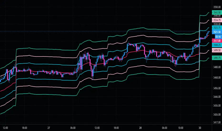
GMS: VWAP with Percent BandsThis is a pretty straight-forward script. I just wanted to see percent bands around the VWAP after looking at the standard deviation bands for a while and even dabbling with keltner channels. This is the cleanest in my opinion. The script is open so feel free to poke around!
The default settings are below, just to confuse 0.25 with 25%.
0.25 = 0.25%
0.5 = 0.50%
0.75 = 0.75%
PS - it's not multi-timeframe yet. That'll come in the next update.
Hope this helps,
Andre
Daily Manipulation Probability Dashboard📜 Summary
Tired of getting stopped out on a "Judas Swing" just before the price moves in your intended direction? This indicator is designed to give you a statistical edge by quantifying the daily manipulation move.
The Daily Manipulation Probability Dashboard analyzes thousands of historical trading days to reveal the probability of the initial "stop-hunt" or "fakeout" move reaching certain percentage levels. It presents this data in a clean, intuitive dashboard right on your chart, helping you make more data-driven decisions about stop-loss placement and entry timing.
🧠 The Core Concept
The logic is simple but powerful. For every trading day, we measure two things:
Amplitude Above Open (AAO): The distance price travels up from the daily open (High - Open).
Amplitude Below Open (ABO): The distance price travels down from the daily open (Open - Low).
The indicator defines the "Manipulation" as the smaller of these two moves. The idea is that this smaller move often acts as a liquidity grab to trap traders before the day's primary, larger move ("Distribution") begins.
This tool focuses exclusively on providing deep statistical insight into this crucial manipulation phase.
🛠️ How to Use This Tool
This dashboard is designed to be a practical part of your daily analysis and trade planning.
1. Smarter Stop-Loss Placement
This is the primary use case. The "Prob. (%)" column tells you the historical chance of the manipulation move being at least a certain size.
Example: If the table shows that for EURUSD, the ≥ 0.25% level has a probability of 30%, you can flip this information: there is a 70% probability that the daily manipulation move will be less than 0.25%.
Action: Placing your stop-loss just beyond a level with a low probability gives you a statistically sound buffer against typical stop-hunts.
2. Entry Timing and Patience
The live arrow (→) shows you where the current day's manipulation falls.
Example: If the arrow is pointing at ≥ 0.10% and you know there is a high probability (e.g., 60%) of the manipulation reaching ≥ 0.20%, you might wait for a deeper pullback before entering, anticipating that the "Judas Swing" hasn't completed yet.
3. Assessing Daily Character
Quickly see if the current day's action is unusual. If the manipulation move is already in a very low probability zone (e.g., > 1.00%), it might indicate that your Bias is wrong, or signal a high-volatility day or a potential trend reversal.
📊 Understanding the Dashboard
Ticker: The top-right shows the current symbol you are analyzing.
→ (Arrow): Points to the row that corresponds to the current, live day's manipulation amplitude.
Manip. Level: The percentage threshold being analyzed (e.g., ≥ 0.20%).
Days Analyzed: The raw count of historical days where the manipulation move met or exceeded this level.
Prob. (%): The key statistic. The cumulative probability of the manipulation move being at least the size of the level.
⚙️ Settings
Position: Choose where you want the dashboard to appear on your chart.
Text Size: Adjust the font size for readability.
Max Historical Days to Analyze: Set the number of past daily candles to include in the statistical analysis. A larger number provides a more robust sample size.
I believe this tool provides a unique, data-driven edge for intraday traders across all markets (Forex, Crypto, Stocks, Indices). Your feedback and suggestions are highly welcome!
- @traderprimez

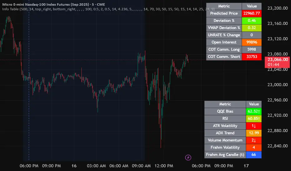
Info TableOverview
The Info Table V1 is a versatile TradingView indicator tailored for intraday futures traders, particularly those focusing on MESM2 (Micro E-mini S&P 500 futures) on 1-minute charts. It presents essential market insights through two customizable tables: the Main Table for predictive and macro metrics, and the New Metrics Table for momentum and volatility indicators. Designed for high-activity sessions like 9:30 AM–11:00 AM CDT, this tool helps traders assess price alignment, sentiment, and risk in real-time. Metrics update dynamically (except weekly COT data), with optional alerts for key conditions like volatility spikes or momentum shifts.
This indicator builds on foundational concepts like linear regression for predictions and adapts open-source elements for enhanced functionality. Gradient code is adapted from TradingView's Color Library. QQE logic is adapted from LuxAlgo's QQE Weighted Oscillator, licensed under CC BY-NC-SA 4.0. The script is released under the Mozilla Public License 2.0.
Key Features
Two Customizable Tables: Positioned independently (e.g., top-right for Main, bottom-right for New Metrics) with toggle options to show/hide for a clutter-free chart.
Gradient Coloring: User-defined high/low colors (default green/red) for quick visual interpretation of extremes, such as overbought/oversold or high volatility.
Arrows for Directional Bias: In the New Metrics Table, up (↑) or down (↓) arrows appear in value cells based on metric thresholds (top/bottom 25% of range), indicating bullish/high or bearish/low conditions.
Consensus Highlighting: The New Metrics Table's title cells ("Metric" and "Value") turn green if all arrows are ↑ (strong bullish consensus), red if all are ↓ (strong bearish consensus), or gray otherwise.
Predicted Price Plot: Optional line (default blue) overlaying the ML-predicted price for visual comparison with actual price action.
Alerts: Notifications for high/low Frahm Volatility (≥8 or ≤3) and QQE Bias crosses (bullish/bearish momentum shifts).
Main Table Metrics
This table focuses on predictive, positional, and macro insights:
ML-Predicted Price: A linear regression forecast using normalized price, volume, and RSI over a customizable lookback (default 500 bars). Gradient scales from low (red) to high (green) relative to the current price ± threshold (default 100 points).
Deviation %: Percentage difference between current price and predicted price. Gradient highlights extremes (±0.5% default threshold), signaling potential overextensions.
VWAP Deviation %: Percentage difference from Volume Weighted Average Price (VWAP). Gradient indicates if price is above (green) or below (red) fair value (±0.5% default).
FRED UNRATE % Change: Percentage change in U.S. unemployment rate (via FRED data). Cell turns red for increases (economic weakness), green for decreases (strength), gray if zero or disabled.
Open Interest: Total open MESM2 futures contracts. Gradient scales from low (red) to high (green) up to a hardcoded 300,000 threshold, reflecting market participation.
COT Commercial Long/Short: Weekly Commitment of Traders data for commercial positions. Long cell green if longs > shorts (bullish institutional sentiment); Short cell red if shorts > longs (bearish); gray otherwise.
New Metrics Table Metrics
This table emphasizes technical momentum and volatility, with arrows for quick bias assessment:
QQE Bias: Smoothed RSI vs. trailing stop (default length 14, factor 4.236, smooth 5). Green for bullish (RSI > stop, ↑ arrow), red for bearish (RSI < stop, ↓ arrow), gray for neutral.
RSI: Relative Strength Index (default period 14). Gradient from oversold (red, <30 + threshold offset, ↓ arrow if ≤40) to overbought (green, >70 - offset, ↑ arrow if ≥60).
ATR Volatility: Score (1–20) based on Average True Range (default period 14, lookback 50). High scores (green, ↑ if ≥15) signal swings; low (red, ↓ if ≤5) indicate calm.
ADX Trend: Average Directional Index (default period 14). Gradient from weak (red, ↓ if ≤0.25×25 threshold) to strong trends (green, ↑ if ≥0.75×25).
Volume Momentum: Score (1–20) comparing current to historical volume (lookback 50). High (green, ↑ if ≥15) suggests pressure; low (red, ↓ if ≤5) implies weakness.
Frahm Volatility: Score (1–20) from true range over a window (default 24 hours, multiplier 9). Dynamic gradient (green/red/yellow); ↑ if ≥7.5, ↓ if ≤2.5.
Frahm Avg Candle (Ticks): Average candle size in ticks over the window. Blue gradient (or dynamic green/red/yellow); ↑ if ≥0.75 percentile, ↓ if ≤0.25.
Arrows trigger on metric-specific logic (e.g., RSI ≥60 for ↑), providing directional cues without strict color ties.
Customization Options
Adapt the indicator to your strategy:
ML Inputs: Lookback (10–5000 bars) and RSI period (2+) for prediction sensitivity—shorter for volatility, longer for trends.
Timeframes: Individual per metric (e.g., 1H for QQE Bias to match higher frames; blank for chart timeframe).
Thresholds: Adjust gradients and arrows (e.g., Deviation 0.1–5%, ADX 0–100, RSI overbought/oversold).
QQE Settings: Length, factor, and smooth for fine-tuned momentum.
Data Toggles: Enable/disable FRED, Open Interest, COT for focus (e.g., disable macro for pure intraday).
Frahm Options: Window hours (1+), scale multiplier (1–10), dynamic colors for avg candle.
Plot/Table: Line color, positions, gradients, and visibility.
Ideal Use Case
Perfect for MESM2 scalpers and trend traders. Use the Main Table for entry confirmation via predicted deviations and institutional positioning. Leverage the New Metrics Table arrows for short-term signals—enter bullish on green consensus (all ↑), avoid chop on low volatility. Set alerts to catch shifts without constant monitoring.
Why It's Valuable
Info Table V1 consolidates diverse metrics into actionable visuals, answering critical questions: Is price mispriced? Is momentum aligning? Is volatility manageable? With real-time updates, consensus highlights, and extensive customization, it enhances precision in fast markets, reducing guesswork for confident trades.
Note: Optimized for futures; some metrics (OI, COT) unavailable on non-futures symbols. Test on demo accounts. No financial advice—use at your own risk.
The provided script reuses open-source elements from TradingView's Color Library and LuxAlgo's QQE Weighted Oscillator, as noted in the script comments and description. Credits are appropriately given in both the description and code comments, satisfying the requirement for attribution.
Regarding significant improvements and proportion:
The QQE logic comprises approximately 15 lines of code in a script exceeding 400 lines, representing a small proportion (<5%).
Adaptations include integration with multi-timeframe support via request.security, user-customizable inputs for length, factor, and smooth, and application within a broader table-based indicator for momentum bias display (with color gradients, arrows, and alerts). This extends the original QQE beyond standalone oscillator use, incorporating it as one of seven metrics in the New Metrics Table for confluence analysis (e.g., consensus highlighting when all metrics align). These are functional enhancements, not mere stylistic or variable changes.
The Color Library usage is via official import (import TradingView/Color/1 as Color), leveraging built-in gradient functions without copying code, and applied to enhance visual interpretation across multiple metrics.
The script complies with the rules: reused code is minimal, significantly improved through integration and expansion, and properly credited. It qualifies for open-source publication under the Mozilla Public License 2.0, as stated.
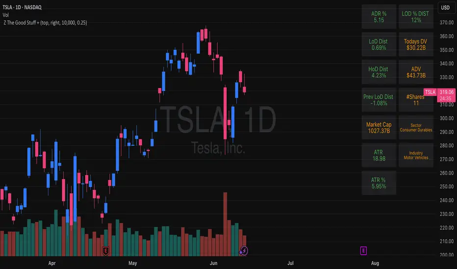
Z The Good Stuff +I created this script to have a couple datapoints that I want to look at when going through charts to find trade ideas. Qullamaggie is one of my biggest inspirations and I built in a couple of his concepts with a touch to help me with sizing properly, all explained below:
Box 1: ADR %, Average Daily Range, gives and indication of how volatile the stock is. It uses the 20 day average % move of the current stock on the chart.
Box 2: LOD Distance, low of day distance is a quality of life element I created. It calculates the low for the current candle and color codes it red or green depending on if it's higher or lower than the daily ADR. The logic is that if a stock has an average speed, buying on a setup it is preferred if the stop distance (assuming a low of day stop) should be less than the ADR to improve the odds of more upside.
Box 3: Todays DV, this shows a rough estimate of how much money was traded on the particular day.
Box 4: ADV 20 days, similar to above this shows the 20 day $ traded average. The point to look at it is to have a better idea what position size is possible to not get stuck in something too illiquid.
Box 5: Market cap, just shows the market cap of the stock to know what size the company is.
Box 6: Number of shares, this is an additional quality of life aspect. If using low of day stops, this part calculates based on the users' inputted portfolio size and portfolio risk preference and then calculates how many stocks to buy to stay within the risk parameters. It is obviously not a sole decision making parameter nor does it guarantee any execution, but if a stock is showing an entry you want to take you can use the number of shares to help you know how many to buy. The preset is a portfolio of 10000 and a risk of 0.25%. This means that the number of shares to buy will be at the current price with lod stop that would result in a 0.25% portfolio loss. OF COURSE the actual loss depends on the execution and if the user places a stop loss order.
Hope you find it useful and feel free to give feedback! Cheers!
Machine Learning: Lorentzian Classification█ OVERVIEW
A Lorentzian Distance Classifier (LDC) is a Machine Learning classification algorithm capable of categorizing historical data from a multi-dimensional feature space. This indicator demonstrates how Lorentzian Classification can also be used to predict the direction of future price movements when used as the distance metric for a novel implementation of an Approximate Nearest Neighbors (ANN) algorithm.
█ BACKGROUND
In physics, Lorentzian space is perhaps best known for its role in describing the curvature of space-time in Einstein's theory of General Relativity (2). Interestingly, however, this abstract concept from theoretical physics also has tangible real-world applications in trading.
Recently, it was hypothesized that Lorentzian space was also well-suited for analyzing time-series data (4), (5). This hypothesis has been supported by several empirical studies that demonstrate that Lorentzian distance is more robust to outliers and noise than the more commonly used Euclidean distance (1), (3), (6). Furthermore, Lorentzian distance was also shown to outperform dozens of other highly regarded distance metrics, including Manhattan distance, Bhattacharyya similarity, and Cosine similarity (1), (3). Outside of Dynamic Time Warping based approaches, which are unfortunately too computationally intensive for PineScript at this time, the Lorentzian Distance metric consistently scores the highest mean accuracy over a wide variety of time series data sets (1).
Euclidean distance is commonly used as the default distance metric for NN-based search algorithms, but it may not always be the best choice when dealing with financial market data. This is because financial market data can be significantly impacted by proximity to major world events such as FOMC Meetings and Black Swan events. This event-based distortion of market data can be framed as similar to the gravitational warping caused by a massive object on the space-time continuum. For financial markets, the analogous continuum that experiences warping can be referred to as "price-time".
Below is a side-by-side comparison of how neighborhoods of similar historical points appear in three-dimensional Euclidean Space and Lorentzian Space:
This figure demonstrates how Lorentzian space can better accommodate the warping of price-time since the Lorentzian distance function compresses the Euclidean neighborhood in such a way that the new neighborhood distribution in Lorentzian space tends to cluster around each of the major feature axes in addition to the origin itself. This means that, even though some nearest neighbors will be the same regardless of the distance metric used, Lorentzian space will also allow for the consideration of historical points that would otherwise never be considered with a Euclidean distance metric.
Intuitively, the advantage inherent in the Lorentzian distance metric makes sense. For example, it is logical that the price action that occurs in the hours after Chairman Powell finishes delivering a speech would resemble at least some of the previous times when he finished delivering a speech. This may be true regardless of other factors, such as whether or not the market was overbought or oversold at the time or if the macro conditions were more bullish or bearish overall. These historical reference points are extremely valuable for predictive models, yet the Euclidean distance metric would miss these neighbors entirely, often in favor of irrelevant data points from the day before the event. By using Lorentzian distance as a metric, the ML model is instead able to consider the warping of price-time caused by the event and, ultimately, transcend the temporal bias imposed on it by the time series.
For more information on the implementation details of the Approximate Nearest Neighbors (ANN) algorithm used in this indicator, please refer to the detailed comments in the source code.
█ HOW TO USE
Below is an explanatory breakdown of the different parts of this indicator as it appears in the interface:
Below is an explanation of the different settings for this indicator:
General Settings:
Source - This has a default value of "hlc3" and is used to control the input data source.
Neighbors Count - This has a default value of 8, a minimum value of 1, a maximum value of 100, and a step of 1. It is used to control the number of neighbors to consider.
Max Bars Back - This has a default value of 2000.
Feature Count - This has a default value of 5, a minimum value of 2, and a maximum value of 5. It controls the number of features to use for ML predictions.
Color Compression - This has a default value of 1, a minimum value of 1, and a maximum value of 10. It is used to control the compression factor for adjusting the intensity of the color scale.
Show Exits - This has a default value of false. It controls whether to show the exit threshold on the chart.
Use Dynamic Exits - This has a default value of false. It is used to control whether to attempt to let profits ride by dynamically adjusting the exit threshold based on kernel regression.
Feature Engineering Settings:
Note: The Feature Engineering section is for fine-tuning the features used for ML predictions. The default values are optimized for the 4H to 12H timeframes for most charts, but they should also work reasonably well for other timeframes. By default, the model can support features that accept two parameters (Parameter A and Parameter B, respectively). Even though there are only 4 features provided by default, the same feature with different settings counts as two separate features. If the feature only accepts one parameter, then the second parameter will default to EMA-based smoothing with a default value of 1. These features represent the most effective combination I have encountered in my testing, but additional features may be added as additional options in the future.
Feature 1 - This has a default value of "RSI" and options are: "RSI", "WT", "CCI", "ADX".
Feature 2 - This has a default value of "WT" and options are: "RSI", "WT", "CCI", "ADX".
Feature 3 - This has a default value of "CCI" and options are: "RSI", "WT", "CCI", "ADX".
Feature 4 - This has a default value of "ADX" and options are: "RSI", "WT", "CCI", "ADX".
Feature 5 - This has a default value of "RSI" and options are: "RSI", "WT", "CCI", "ADX".
Filters Settings:
Use Volatility Filter - This has a default value of true. It is used to control whether to use the volatility filter.
Use Regime Filter - This has a default value of true. It is used to control whether to use the trend detection filter.
Use ADX Filter - This has a default value of false. It is used to control whether to use the ADX filter.
Regime Threshold - This has a default value of -0.1, a minimum value of -10, a maximum value of 10, and a step of 0.1. It is used to control the Regime Detection filter for detecting Trending/Ranging markets.
ADX Threshold - This has a default value of 20, a minimum value of 0, a maximum value of 100, and a step of 1. It is used to control the threshold for detecting Trending/Ranging markets.
Kernel Regression Settings:
Trade with Kernel - This has a default value of true. It is used to control whether to trade with the kernel.
Show Kernel Estimate - This has a default value of true. It is used to control whether to show the kernel estimate.
Lookback Window - This has a default value of 8 and a minimum value of 3. It is used to control the number of bars used for the estimation. Recommended range: 3-50
Relative Weighting - This has a default value of 8 and a step size of 0.25. It is used to control the relative weighting of time frames. Recommended range: 0.25-25
Start Regression at Bar - This has a default value of 25. It is used to control the bar index on which to start regression. Recommended range: 0-25
Display Settings:
Show Bar Colors - This has a default value of true. It is used to control whether to show the bar colors.
Show Bar Prediction Values - This has a default value of true. It controls whether to show the ML model's evaluation of each bar as an integer.
Use ATR Offset - This has a default value of false. It controls whether to use the ATR offset instead of the bar prediction offset.
Bar Prediction Offset - This has a default value of 0 and a minimum value of 0. It is used to control the offset of the bar predictions as a percentage from the bar high or close.
Backtesting Settings:
Show Backtest Results - This has a default value of true. It is used to control whether to display the win rate of the given configuration.
█ WORKS CITED
(1) R. Giusti and G. E. A. P. A. Batista, "An Empirical Comparison of Dissimilarity Measures for Time Series Classification," 2013 Brazilian Conference on Intelligent Systems, Oct. 2013, DOI: 10.1109/bracis.2013.22.
(2) Y. Kerimbekov, H. Ş. Bilge, and H. H. Uğurlu, "The use of Lorentzian distance metric in classification problems," Pattern Recognition Letters, vol. 84, 170–176, Dec. 2016, DOI: 10.1016/j.patrec.2016.09.006.
(3) A. Bagnall, A. Bostrom, J. Large, and J. Lines, "The Great Time Series Classification Bake Off: An Experimental Evaluation of Recently Proposed Algorithms." ResearchGate, Feb. 04, 2016.
(4) H. Ş. Bilge, Yerzhan Kerimbekov, and Hasan Hüseyin Uğurlu, "A new classification method by using Lorentzian distance metric," ResearchGate, Sep. 02, 2015.
(5) Y. Kerimbekov and H. Şakir Bilge, "Lorentzian Distance Classifier for Multiple Features," Proceedings of the 6th International Conference on Pattern Recognition Applications and Methods, 2017, DOI: 10.5220/0006197004930501.
(6) V. Surya Prasath et al., "Effects of Distance Measure Choice on KNN Classifier Performance - A Review." .
█ ACKNOWLEDGEMENTS
@veryfid - For many invaluable insights, discussions, and advice that helped to shape this project.
@capissimo - For open sourcing his interesting ideas regarding various KNN implementations in PineScript, several of which helped inspire my original undertaking of this project.
@RikkiTavi - For many invaluable physics-related conversations and for his helping me develop a mechanism for visualizing various distance algorithms in 3D using JavaScript
@jlaurel - For invaluable literature recommendations that helped me to understand the underlying subject matter of this project.
@annutara - For help in beta-testing this indicator and for sharing many helpful ideas and insights early on in its development.
@jasontaylor7 - For helping to beta-test this indicator and for many helpful conversations that helped to shape my backtesting workflow
@meddymarkusvanhala - For helping to beta-test this indicator
@dlbnext - For incredibly detailed backtesting testing of this indicator and for sharing numerous ideas on how the user experience could be improved.
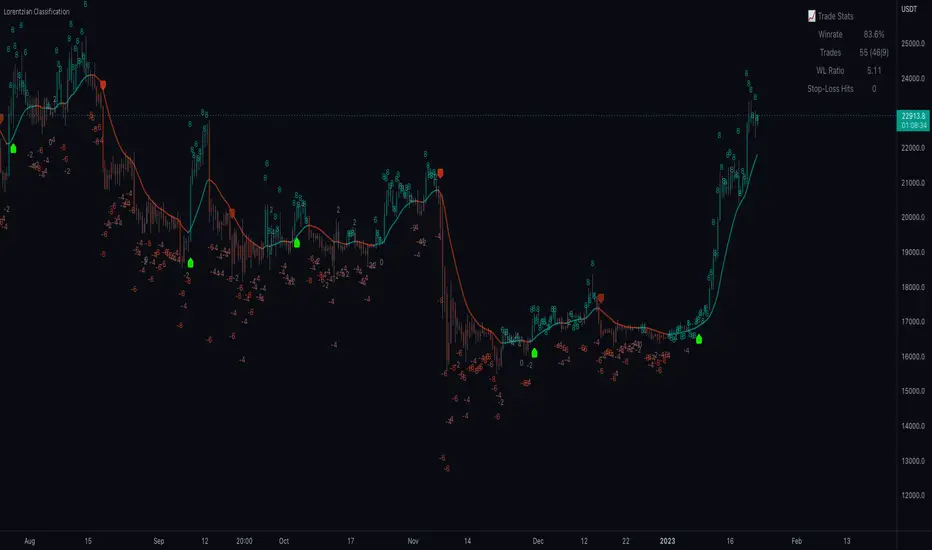
Volatility Calculator for Daily Top and Bottom RangeWith the usage of ATR, applied on the close of the daily candle, I am calculated the volatility channels for the TOP and BOTTOM
Based on this logic, we can estimate, with a huge confidence factor, where the prices are going to be compressed for the trading day.
Having said that, lets take a look at the data gathered among the most important financial markets:
SPX
TOP CROSSES : 2116
BOT CROSSES : 1954
Total Daily Candles : 18908
Occurance ratio = 0.215
NDX
TOP CROSSES : 1212
BOT CROSSES : 1183
Total Daily Candles : 9386
Occurance ratio = 0.255
DIA
TOP CROSSES : 759
BOT CROSSES : 769
Total Daily Candles : 6109
Occurance ratio = 0.25
DXY
TOP CROSSES : 1597
BOT CROSSES : 1598
Total Daily Candles : 13156
Occurance ratio = 0.243
DAX
TOP CROSSES : 1878
BOT CROSSES : 1848
Total Daily Candles : 13155
Occurance ratio = 0.283
BTC USD
TOP CROSSES : 416
BOT CROSSES : 417
Total Daily Candles : 4290
Occurance ratio = 0.194
ETH USD
TOP CROSSES : 247
BOT CROSSES : 268
Total Daily Candles : 2452
Occurance ratio = 0.21
EUR USD
TOP CROSSES : 820
BOT CROSSES : 805
Total Daily Candles : 7489
Occurance ratio = 0.217
GOLD
TOP CROSSES : 1722
BOT CROSSES : 1569
Total Daily Candles : 13747
Occurance ratio = 0.239
USOIL
TOP CROSSES : 1077
BOT CROSSES : 1089
Total Daily Candles : 10231
Occurance ratio = 0.212
US 10Y
TOP CROSSES : 1302
BOT CROSSES : 1365
Total Daily Candles : 9075
Occurance ratio = 0.294
Based on this, we can assume with a very high confidence ( 70-80%) that the market is going to stay, within the range created from the BOT and TOP ATR points.

Closed Form Distance VolatilityIntroduction
Calculating distances in signal processing/statistics/time-series analysis imply measuring the distance between two probability distribution, i am not really familiar with distances but since some formulas are in closed form they can be easily used for volatility estimation. This volatility indicator will use three methods originally made to measure the distance of gaussian copulas, using those methods for volatility estimation is fairly easy and provide a different approach to statistical dispersion.
The indicator have a length parameter and a method parameter to select the method used for volatility estimation, i describe each methods below.
Hellinger Method
Each method will use the rolling sum of the low price and the rolling sum of the high price instead of probability distributions. The Hellinger method have many application from the measurement of distances to the use as a cost function for neural networks.
Its closed form is defined as the square root of 1 - a^0.25b^0.25/(0.5a + 0.5b)^0.5 where a and b are both positive series. In our indicator a is the rolling sum of the high price and b the rolling sum of the low price. This method give a classic estimation of volatility.
Bhattacharyya Method
The Bhattacharyya method is another method who use a natural logarithm, this method can visually filter small volatility variation. It is defined as 0.5 * log((0.5a+0.5b)/√(ab)) .
Wasserstein Method
This method was originally using a trimmed mean for its calculation. The original method is defined as the square of the trimmed mean of a + b - 2√(a^0.5ba^0.5) , a median has been used instead of a trimmed mean for efficiency sake, both central tendency estimators are robust to outliers.
Conclusion
I showed that closed form formulas for distance calculation could be derived into volatility estimators with different properties. They could be used with series in a range of (0,1) to provide a smoothing variable for exponential smoothing.

order block new 113/// This work is licensed under a Attribution-NonCommercial-ShareAlike 4.0 International (CC BY-NC-SA 4.0) creativecommons.org
// © RUDYBANK INDICATOR - formerly know as RUDY INDICATOR
//@version=5
indicator("Price Action Concepts ", shorttitle = "RUDYINDICATOR-V1
- Price Action RUDYINDICATOR ", overlay = true, max_lines_count = 500, max_labels_count = 500, max_boxes_count = 500, max_bars_back = 500, max_polylines_count = 100)
//-----------------------------------------------------------------------------{
//Boolean set
//-----------------------------------------------------------------------------{
s_BOS = 0
s_CHoCH = 1
i_BOS = 2
i_CHoCH = 3
i_pp_CHoCH = 4
green_candle = 5
red_candle = 6
s_CHoCHP = 7
i_CHoCHP = 8
boolean =
array.from(
false
, false
, false
, false
, false
, false
, false
, false
, false
)
//-----------------------------------------------------------------------------{
// User inputs
//-----------------------------------------------------------------------------{
show_swing_ms = input.string ("All" , "Swing        " , inline = "1", group = "MARKET STRUCTURE" , options = )
show_internal_ms = input.string ("All" , "Internal     " , inline = "2", group = "MARKET STRUCTURE" , options = )
internal_r_lookback = input.int (5 , "" , inline = "2", group = "MARKET STRUCTURE" , minval = 2)
swing_r_lookback = input.int (50 , "" , inline = "1", group = "MARKET STRUCTURE" , minval = 2)
ms_mode = input.string ("Manual" , "Market Structure Mode" , inline = "a", group = "MARKET STRUCTURE" , tooltip = " Use selected lenght\n Use automatic lenght" ,options = )
show_mtf_str = input.bool (true , "MTF Scanner" , inline = "9", group = "MARKET STRUCTURE" , tooltip = "Display Multi-Timeframe Market Structure Trend Directions. Green = Bullish. Red = Bearish")
show_eql = input.bool (false , "Show EQH/EQL" , inline = "6", group = "MARKET STRUCTURE")
plotcandle_bool = input.bool (false , "Plotcandle" , inline = "3", group = "MARKET STRUCTURE" , tooltip = "Displays a cleaner colored candlestick chart in place of the default candles. (requires hiding the current ticker candles)")
barcolor_bool = input.bool (false , "Bar Color" , inline = "4", group = "MARKET STRUCTURE" , tooltip = "Color the candle bodies according to market strucutre trend")
i_ms_up_BOS = input.color (#089981 , "" , inline = "2", group = "MARKET STRUCTURE")
i_ms_dn_BOS = input.color (#f23645 , "" , inline = "2", group = "MARKET STRUCTURE")
s_ms_up_BOS = input.color (#089981 , "" , inline = "1", group = "MARKET STRUCTURE")
s_ms_dn_BOS = input.color (#f23645 , "" , inline = "1", group = "MARKET STRUCTURE")
lvl_daily = input.bool (false , "Day   " , inline = "1", group = "HIGHS & LOWS MTF")
lvl_weekly = input.bool (false , "Week " , inline = "2", group = "HIGHS & LOWS MTF")
lvl_monthly = input.bool (false , "Month" , inline = "3", group = "HIGHS & LOWS MTF")
lvl_yearly = input.bool (false , "Year  " , inline = "4", group = "HIGHS & LOWS MTF")
css_d = input.color (color.blue , "" , inline = "1", group = "HIGHS & LOWS MTF")
css_w = input.color (color.blue , "" , inline = "2", group = "HIGHS & LOWS MTF")
css_m = input.color (color.blue , "" , inline = "3", group = "HIGHS & LOWS MTF")
css_y = input.color (color.blue , "" , inline = "4", group = "HIGHS & LOWS MTF")
s_d = input.string ('⎯⎯⎯' , '' , inline = '1', group = 'HIGHS & LOWS MTF' , options = )
s_w = input.string ('⎯⎯⎯' , '' , inline = '2', group = 'HIGHS & LOWS MTF' , options = )
s_m = input.string ('⎯⎯⎯' , '' , inline = '3', group = 'HIGHS & LOWS MTF' , options = )
s_y = input.string ('⎯⎯⎯' , '' , inline = '4', group = 'HIGHS & LOWS MTF' , options = )
ob_show = input.bool (true , "Show Last    " , inline = "1", group = "VOLUMETRIC ORDER BLOCKS" , tooltip = "Display volumetric order blocks on the chart \n\n Ammount of volumetric order blocks to show")
ob_num = input.int (5 , "" , inline = "1", group = "VOLUMETRIC ORDER BLOCKS" , tooltip = "Orderblocks number", minval = 1, maxval = 10)
ob_metrics_show = input.bool (true , "Internal Buy/Sell Activity" , inline = "2", group = "VOLUMETRIC ORDER BLOCKS" , tooltip = "Display volume metrics that have formed the orderblock")
css_metric_up = input.color (color.new(#089981, 50) , "         " , inline = "2", group = "VOLUMETRIC ORDER BLOCKS")
css_metric_dn = input.color (color.new(#f23645 , 50) , "" , inline = "2", group = "VOLUMETRIC ORDER BLOCKS")
ob_swings = input.bool (false , "Swing Order Blocks" , inline = "a", group = "VOLUMETRIC ORDER BLOCKS" , tooltip = "Display swing volumetric order blocks")
css_swing_up = input.color (color.new(color.gray , 90) , "                 " , inline = "a", group = "VOLUMETRIC ORDER BLOCKS")
css_swing_dn = input.color (color.new(color.silver, 90) , "" , inline = "a", group = "VOLUMETRIC ORDER BLOCKS")
ob_filter = input.string ("None" , "Filtering             " , inline = "d", group = "VOLUMETRIC ORDER BLOCKS" , tooltip = "Filter out volumetric order blocks by BOS/CHoCH/CHoCH+", options = )
ob_mitigation = input.string ("Absolute" , "Mitigation           " , inline = "4", group = "VOLUMETRIC ORDER BLOCKS" , tooltip = "Trigger to remove volumetric order blocks", options = )
ob_pos = input.string ("Precise" , "Positioning          " , inline = "k", group = "VOLUMETRIC ORDER BLOCKS" , tooltip = "Position of the Order Block\n Cover the whole candle\n Cover half candle\n Adjust to volatility\n Same as Accurate but more precise", options = )
use_grayscale = input.bool (false , "Grayscale" , inline = "6", group = "VOLUMETRIC ORDER BLOCKS" , tooltip = "Use gray as basic order blocks color")
use_show_metric = input.bool (true , "Show Metrics" , inline = "7", group = "VOLUMETRIC ORDER BLOCKS" , tooltip = "Show volume associated with the orderblock and his relevance")
use_middle_line = input.bool (true , "Show Middle-Line" , inline = "8", group = "VOLUMETRIC ORDER BLOCKS" , tooltip = "Show mid-line order blocks")
use_overlap = input.bool (true , "Hide Overlap" , inline = "9", group = "VOLUMETRIC ORDER BLOCKS" , tooltip = "Hide overlapping order blocks")
use_overlap_method = input.string ("Previous" , "Overlap Method    " , inline = "Z", group = "VOLUMETRIC ORDER BLOCKS" , tooltip = " Preserve the most recent volumetric order blocks\n\n Preserve the previous volumetric order blocks", options = )
ob_bull_css = input.color (color.new(#089981 , 90) , "" , inline = "1", group = "VOLUMETRIC ORDER BLOCKS")
ob_bear_css = input.color (color.new(#f23645 , 90) , "" , inline = "1", group = "VOLUMETRIC ORDER BLOCKS")
show_acc_dist_zone = input.bool (false , "" , inline = "1", group = "Accumulation And Distribution")
zone_mode = input.string ("Fast" , "" , inline = "1", group = "Accumulation And Distribution" , tooltip = " Find small zone pattern formation\n Find bigger zone pattern formation" ,options = )
acc_css = input.color (color.new(#089981 , 60) , "" , inline = "1", group = "Accumulation And Distribution")
dist_css = input.color (color.new(#f23645 , 60) , "" , inline = "1", group = "Accumulation And Distribution")
show_lbl = input.bool (false , "Show swing point" , inline = "1", group = "High and Low" , tooltip = "Display swing point")
show_mtb = input.bool (false , "Show High/Low/Equilibrium" , inline = "2", group = "High and Low" , tooltip = "Display Strong/Weak High And Low and Equilibrium")
toplvl = input.color (color.red , "Premium Zone   " , inline = "3", group = "High and Low")
midlvl = input.color (color.gray , "Equilibrium Zone" , inline = "4", group = "High and Low")
btmlvl = input.color (#089981 , "Discount Zone    " , inline = "5", group = "High and Low")
fvg_enable = input.bool (false , "        " , inline = "1", group = "FAIR VALUE GAP" , tooltip = "Display fair value gap")
what_fvg = input.string ("FVG" , "" , inline = "1", group = "FAIR VALUE GAP" , tooltip = "Display fair value gap", options = )
fvg_num = input.int (5 , "Show Last  " , inline = "1a", group = "FAIR VALUE GAP" , tooltip = "Number of fvg to show")
fvg_upcss = input.color (color.new(#089981, 80) , "" , inline = "1", group = "FAIR VALUE GAP")
fvg_dncss = input.color (color.new(color.red , 80) , "" , inline = "1", group = "FAIR VALUE GAP")
fvg_extend = input.int (10 , "Extend FVG" , inline = "2", group = "FAIR VALUE GAP" , tooltip = "Extend the display of the FVG.")
fvg_src = input.string ("Close" , "Mitigation  " , inline = "3", group = "FAIR VALUE GAP" , tooltip = " Use the close of the body as trigger\n\n Use the extreme point of the body as trigger", options = )
fvg_tf = input.timeframe ("" , "Timeframe " , inline = "4", group = "FAIR VALUE GAP" , tooltip = "Timeframe of the fair value gap")
t = color.t (ob_bull_css)
invcol = color.new (color.white , 100)
//{----------------------------------------------------------------------------------------------------------------------------------------------}
//{----------------------------------------------------------------------------------------------------------------------------------------------}
//{----------------------------------------------------------------------------------------------------------------------------------------------}
//{----------------------------------------------------------------------------------------------------------------------------------------------}
//{ - UDT }
//{----------------------------------------------------------------------------------------------------------------------------------------------}
//{----------------------------------------------------------------------------------------------------------------------------------------------}
//{----------------------------------------------------------------------------------------------------------------------------------------------}
//{----------------------------------------------------------------------------------------------------------------------------------------------}
type bar
float o = open
float c = close
float h = high
float l = low
float v = volume
int n = bar_index
int t = time
type Zphl
line top
line bottom
label top_label
label bottom_label
bool stopcross
bool sbottomcross
bool itopcross
bool ibottomcross
string txtup
string txtdn
float topy
float bottomy
float topx
float bottomx
float tup
float tdn
int tupx
int tdnx
float itopy
float itopx
float ibottomy
float ibottomx
float uV
float dV
type FVG
box box
line ln
bool bull
float top
float btm
int left
int right
type ms
float p
int n
float l
type msDraw
int n
float p
color css
string txt
bool bull
type obC
float top
float btm
int left
float avg
float dV
float cV
int wM
int blVP
int brVP
int dir
float h
float l
int n
type obD
box ob
box eOB
box blB
box brB
line mL
type zone
chart.point points
float p
int c
int t
type hqlzone
box pbx
box ebx
box lbx
label plb
label elb
label lbl
type ehl
float pt
int t
float pb
int b
type pattern
string found = "None"
bool isfound = false
int period = 0
bool bull = false
type alerts
bool chochswing = false
bool chochplusswing = false
bool swingbos = false
bool chochplus = false
bool choch = false
bool bos = false
bool equal = false
bool ob = false
bool swingob = false
bool zone = false
bool fvg = false
bool obtouch = false
//{----------------------------------------------------------------------------------------------------------------------------------------------}
//{----------------------------------------------------------------------------------------------------------------------------------------------}
//{----------------------------------------------------------------------------------------------------------------------------------------------}
//{----------------------------------------------------------------------------------------------------------------------------------------------}
//{ - End }
//{----------------------------------------------------------------------------------------------------------------------------------------------}
//{----------------------------------------------------------------------------------------------------------------------------------------------}
//{----------------------------------------------------------------------------------------------------------------------------------------------}
//{----------------------------------------------------------------------------------------------------------------------------------------------}
//{----------------------------------------------------------------------------------------------------------------------------------------------}
//{----------------------------------------------------------------------------------------------------------------------------------------------}
//{----------------------------------------------------------------------------------------------------------------------------------------------}
//{----------------------------------------------------------------------------------------------------------------------------------------------}
//{ - General Setup }
//{----------------------------------------------------------------------------------------------------------------------------------------------}
//{----------------------------------------------------------------------------------------------------------------------------------------------}
//{----------------------------------------------------------------------------------------------------------------------------------------------}
//{----------------------------------------------------------------------------------------------------------------------------------------------}
bar b = bar.new()
var pattern p = pattern.new()
alerts blalert = alerts.new()
alerts bralert = alerts.new()
if p.isfound
p.period += 1
if p.period == 50
p.period := 0
p.found := "None"
p.isfound := false
p.bull := na
switch
b.c > b.o => boolean.set(green_candle, true)
b.c < b.o => boolean.set(red_candle , true)
f_zscore(src, lookback) =>
(src - ta.sma(src, lookback)) / ta.stdev(src, lookback)
var int iLen = internal_r_lookback
var int sLen = swing_r_lookback
vv = f_zscore(((close - close ) / close ) * 100,iLen)
if ms_mode == "Dynamic"
switch
vv >= 1.5 or vv <= -1.5 => iLen := 10
vv >= 1.6 or vv <= -1.6 => iLen := 9
vv >= 1.7 or vv <= -1.7 => iLen := 8
vv >= 1.8 or vv <= -1.8 => iLen := 7
vv >= 1.9 or vv <= -1.9 => iLen := 6
vv >= 2.0 or vv <= -2.0 => iLen := 5
=> iLen
var msline = array.new(0)
iH = ta.pivothigh(high, iLen, iLen)
sH = ta.pivothigh(high, sLen, sLen)
iL = ta.pivotlow (low , iLen, iLen)
sL = ta.pivotlow (low , sLen, sLen)
//{----------------------------------------------------------------------------------------------------------------------------------------------}
//{----------------------------------------------------------------------------------------------------------------------------------------------}
//{----------------------------------------------------------------------------------------------------------------------------------------------}
//{----------------------------------------------------------------------------------------------------------------------------------------------}
//{ - End }
//{----------------------------------------------------------------------------------------------------------------------------------------------}
//{----------------------------------------------------------------------------------------------------------------------------------------------}
//{----------------------------------------------------------------------------------------------------------------------------------------------}
//{----------------------------------------------------------------------------------------------------------------------------------------------}
//{----------------------------------------------------------------------------------------------------------------------------------------------}
//{----------------------------------------------------------------------------------------------------------------------------------------------}
//{----------------------------------------------------------------------------------------------------------------------------------------------}
//{----------------------------------------------------------------------------------------------------------------------------------------------}
//{ - ARRAYS }
//{----------------------------------------------------------------------------------------------------------------------------------------------}
//{----------------------------------------------------------------------------------------------------------------------------------------------}
//{----------------------------------------------------------------------------------------------------------------------------------------------}
//{----------------------------------------------------------------------------------------------------------------------------------------------}
hl () =>
= request.security(syminfo.tickerid , 'D' , hl() , lookahead = barmerge.lookahead_on)
= request.security(syminfo.tickerid , 'W' , hl() , lookahead = barmerge.lookahead_on)
= request.security(syminfo.tickerid , 'M' , hl() , lookahead = barmerge.lookahead_on)
= request.security(syminfo.tickerid , '12M', hl() , lookahead = barmerge.lookahead_on)
lstyle(style) =>
out = switch style
'⎯⎯⎯' => line.style_solid
'----' => line.style_dashed
'····' => line.style_dotted
mtfphl(h, l ,tf ,css, pdhl_style) =>
var line hl = line.new(
na
, na
, na
, na
, xloc = xloc.bar_time
, color = css
, style = lstyle(pdhl_style)
)
var line ll = line.new(
na
, na
, na
, na
, xloc = xloc.bar_time
, color = css
, style = lstyle(pdhl_style)
)
var label lbl = label.new(
na
, na
, xloc = xloc.bar_time
, text = str.format('P{0}L', tf)
, color = invcol
, textcolor = css
, size = size.small
, style = label.style_label_left
)
var label hlb = label.new(
na
, na
, xloc = xloc.bar_time
, text = str.format('P{0}H', tf)
, color = invcol
, textcolor = css
, size = size.small
, style = label.style_label_left
)
hy = ta.valuewhen(h != h , h , 1)
hx = ta.valuewhen(h == high , time , 1)
ly = ta.valuewhen(l != l , l , 1)
lx = ta.valuewhen(l == low , time , 1)
if barstate.islast
extension = time + (time - time ) * 50
line.set_xy1(hl , hx , hy)
line.set_xy2(hl , extension , hy)
label.set_xy(hlb, extension , hy)
line.set_xy1(ll , lx , ly)
line.set_xy2(ll , extension , ly)
label.set_xy(lbl, extension , ly)
if lvl_daily
mtfphl(pdh , pdl , 'D' , css_d, s_d)
if lvl_weekly
mtfphl(pwh , pwl , 'W' , css_w, s_w)
if lvl_monthly
mtfphl(pmh , pml, 'M' , css_m, s_m)
if lvl_yearly
mtfphl(pyh , pyl , '12M', css_y, s_y)
//{----------------------------------------------------------------------------------------------------------------------------------------------}
//{----------------------------------------------------------------------------------------------------------------------------------------------}
//{----------------------------------------------------------------------------------------------------------------------------------------------}
//{----------------------------------------------------------------------------------------------------------------------------------------------}
//{ - End }
//{----------------------------------------------------------------------------------------------------------------------------------------------}
//{----------------------------------------------------------------------------------------------------------------------------------------------}
//{----------------------------------------------------------------------------------------------------------------------------------------------}
//{----------------------------------------------------------------------------------------------------------------------------------------------}
//{----------------------------------------------------------------------------------------------------------------------------------------------}
//{----------------------------------------------------------------------------------------------------------------------------------------------}
//{----------------------------------------------------------------------------------------------------------------------------------------------}
//{----------------------------------------------------------------------------------------------------------------------------------------------}
//{ - Market Structure }
//{----------------------------------------------------------------------------------------------------------------------------------------------}
//{----------------------------------------------------------------------------------------------------------------------------------------------}
//{----------------------------------------------------------------------------------------------------------------------------------------------}
//{----------------------------------------------------------------------------------------------------------------------------------------------}
method darkcss(color css, float factor, bool bull) =>
blue = color.b(css) * (1 - factor)
red = color.r(css) * (1 - factor)
green = color.g(css) * (1 - factor)
color.rgb(red, green, blue, 0)
method f_line(msDraw d, size, style) =>
var line id = na
var label lbl = na
id := line.new(
d.n
, d.p
, b.n
, d.p
, color = d.css
, width = 1
, style = style
)
if msline.size() >= 250
line.delete(msline.shift())
msline.push(id)
lbl := label.new(
int(math.avg(d.n, b.n))
, d.p
, d.txt
, color = invcol
, textcolor = d.css
, style = d.bull ? label.style_label_down : label.style_label_up
, size = size
, text_font_family = font.family_monospace
)
structure(bool mtf) =>
msDraw drw = na
bool isdrw = false
bool isdrwS = false
var color css = na
var color icss = na
var int itrend = 0
var int trend = 0
bool bull_ob = false
bool bear_ob = false
bool s_bull_ob = false
bool s_bear_ob = false
n = bar_index
var ms up = ms.new(
array.new()
, array.new< int >()
, array.new()
)
var ms dn = ms.new(
array.new()
, array.new< int >()
, array.new()
)
var ms sup = ms.new(
array.new()
, array.new< int >()
, array.new()
)
var ms sdn = ms.new(
array.new()
, array.new< int >()
, array.new()
)
switch show_swing_ms
"All" => boolean.set(s_BOS , true ), boolean.set(s_CHoCH, true ) , boolean.set(s_CHoCHP, true )
"CHoCH" => boolean.set(s_BOS , false), boolean.set(s_CHoCH, true ) , boolean.set(s_CHoCHP, false )
"CHoCH+" => boolean.set(s_BOS , false), boolean.set(s_CHoCH, false) , boolean.set(s_CHoCHP, true )
"BOS" => boolean.set(s_BOS , true ), boolean.set(s_CHoCH, false) , boolean.set(s_CHoCHP, false )
"None" => boolean.set(s_BOS , false), boolean.set(s_CHoCH, false) , boolean.set(s_CHoCHP, false )
=> na
switch show_internal_ms
"All" => boolean.set(i_BOS, true ), boolean.set(i_CHoCH, true ), boolean.set(i_CHoCHP, true )
"CHoCH" => boolean.set(i_BOS, false), boolean.set(i_CHoCH, true ), boolean.set(i_CHoCHP, false)
"CHoCH+" => boolean.set(i_BOS, false), boolean.set(i_CHoCH, false ), boolean.set(i_CHoCHP, true )
"BOS" => boolean.set(i_BOS, true ), boolean.set(i_CHoCH, false ), boolean.set(i_CHoCHP, false)
"None" => boolean.set(i_BOS, false), boolean.set(i_CHoCH, false ), boolean.set(i_CHoCHP, false)
=> na
switch
iH =>
up.p.unshift(b.h )
up.l.unshift(b.h )
up.n.unshift(n )
iL =>
dn.p.unshift(b.l )
dn.l.unshift(b.l )
dn.n.unshift(n )
sL =>
sdn.p.unshift(b.l )
sdn.l.unshift(b.l )
sdn.n.unshift(n )
sH =>
sup.p.unshift(b.h )
sup.l.unshift(b.h )
sup.n.unshift(n )
// INTERNAL BULLISH STRUCTURE
if up.p.size() > 0 and dn.l.size() > 1
if ta.crossover(b.c, up.p.first())
bool CHoCH = na
string txt = na
if itrend < 0
CHoCH := true
switch
not CHoCH =>
txt := "BOS"
css := i_ms_up_BOS
blalert.bos := true
if boolean.get(i_BOS) and mtf == false and na(drw)
isdrw := true
drw := msDraw.new(
up.n.first()
, up.p.first()
, i_ms_up_BOS
, txt
, true
)
CHoCH =>
dn.l.first() > dn.l.get(1) ? blalert.chochplus : blalert.choch
txt := dn.l.first() > dn.l.get(1) ? "CHoCH+" : "CHoCH"
css := i_ms_up_BOS.darkcss(0.25, true)
if (dn.l.first() > dn.l.get(1) ? boolean.get(i_CHoCHP) : boolean.get(i_CHoCH)) and mtf == false and na(drw)
isdrw := true
drw := msDraw.new(
up.n.first()
, up.p.first()
, i_ms_up_BOS.darkcss(0.25, true)
, txt
, true
)
if mtf == false
switch
ob_filter == "None" => bull_ob := true
ob_filter == "BOS" and txt == "BOS" => bull_ob := true
ob_filter == "CHoCH" and txt == "CHoCH" => bull_ob := true
ob_filter == "CHoCH+" and txt == "CHoCH+" => bull_ob := true
itrend := 1
up.n.clear()
up.p.clear()
// INTERNAL BEARISH STRUCTURE
if dn.p.size() > 0 and up.l.size() > 1
if ta.crossunder(b.c, dn.p.first())
bool CHoCH = na
string txt = na
if itrend > 0
CHoCH := true
switch
not CHoCH =>
bralert.bos := true
txt := "BOS"
css := i_ms_dn_BOS
if boolean.get(i_BOS) and mtf == false and na(drw)
isdrw := true
drw := msDraw.new(
dn.n.first()
, dn.p.first()
, i_ms_dn_BOS
, txt
, false
)
CHoCH =>
if up.l.first() < up.l.get(1)
bralert.chochplus := true
else
bralert.choch := true
txt := up.l.first() < up.l.get(1) ? "CHoCH+" : "CHoCH"
css := i_ms_dn_BOS.darkcss(0.25, false)
if (up.l.first() < up.l.get(1) ? boolean.get(i_CHoCHP) : boolean.get(i_CHoCH)) and mtf == false and na(drw)
isdrw := true
drw := msDraw.new(
dn.n.first()
, dn.p.first()
, i_ms_dn_BOS.darkcss(0.25, false)
, txt
, false
)
if mtf == false
switch
ob_filter == "None" => bear_ob := true
ob_filter == "BOS" and txt == "BOS" => bear_ob := true
ob_filter == "CHoCH" and txt == "CHoCH" => bear_ob := true
ob_filter == "CHoCH+" and txt == "CHoCH+" => bear_ob := true
itrend := -1
dn.n.clear()
dn.p.clear()
// SWING BULLISH STRUCTURE
if sup.p.size() > 0 and sdn.l.size() > 1
if ta.crossover(b.c, sup.p.first())
bool CHoCH = na
string txt = na
if trend < 0
CHoCH := true
switch
not CHoCH =>
blalert.swingbos := true
txt := "BOS"
icss := s_ms_up_BOS
if boolean.get(s_BOS) and mtf == false and na(drw)
isdrwS := true
drw := msDraw.new(
sup.n.first()
, sup.p.first()
, s_ms_up_BOS
, txt
, true
)
CHoCH =>
if sdn.l.first() > sdn.l.get(1)
blalert.chochplusswing := true
else
blalert.chochswing := true
txt := sdn.l.first() > sdn.l.get(1) ? "CHoCH+" : "CHoCH"
icss := s_ms_up_BOS.darkcss(0.25, true)
if (sdn.l.first() > sdn.l.get(1) ? boolean.get(s_CHoCHP) : boolean.get(s_CHoCH)) and mtf == false and na(drw)
isdrwS := true
drw := msDraw.new(
sup.n.first()
, sup.p.first()
, s_ms_up_BOS.darkcss(0.25, true)
, txt
, true
)
if mtf == false
switch
ob_filter == "None" => s_bull_ob := true
ob_filter == "BOS" and txt == "BOS" => s_bull_ob := true
ob_filter == "CHoCH" and txt == "CHoCH" => s_bull_ob := true
ob_filter == "CHoCH+" and txt == "CHoCH+" => s_bull_ob := true
trend := 1
sup.n.clear()
sup.p.clear()
// SWING BEARISH STRUCTURE
if sdn.p.size() > 0 and sup.l.size() > 1
if ta.crossunder(b.c, sdn.p.first())
bool CHoCH = na
string txt = na
if trend > 0
CHoCH := true
switch
not CHoCH =>
bralert.swingbos := true
txt := "BOS"
icss := s_ms_dn_BOS
if boolean.get(s_BOS) and mtf == false and na(drw)
isdrwS := true
drw := msDraw.new(
sdn.n.first()
, sdn.p.first()
, s_ms_dn_BOS
, txt
, false
)
CHoCH =>
if sup.l.first() < sup.l.get(1)
bralert.chochplusswing := true
else
bralert.chochswing := true
txt := sup.l.first() < sup.l.get(1) ? "CHoCH+" : "CHoCH"
icss := s_ms_dn_BOS.darkcss(0.25, false)
if (sup.l.first() < sup.l.get(1) ? boolean.get(s_CHoCHP) : boolean.get(s_CHoCH)) and mtf == false and na(drw)
isdrwS := true
drw := msDraw.new(
sdn.n.first()
, sdn.p.first()
, s_ms_dn_BOS.darkcss(0.25, false)
, txt
, false
)
if mtf == false
switch
ob_filter == "None" => s_bear_ob := true
ob_filter == "BOS" and txt == "BOS" => s_bear_ob := true
ob_filter == "CHoCH" and txt == "CHoCH" => s_bear_ob := true
ob_filter == "CHoCH+" and txt == "CHoCH+" => s_bear_ob := true
trend := -1
sdn.n.clear()
sdn.p.clear()
= structure(false)
if isdrw
f_line(drw, size.small, line.style_dashed)
if isdrwS
f_line(drw, size.small, line.style_solid)
= request.security("", "15" , structure(true))
= request.security("", "60" , structure(true))
= request.security("", "240" , structure(true))
= request.security("", "1440" , structure(true))
if show_mtf_str
var tab = table.new(position = position.top_right, columns = 10, rows = 10, bgcolor = na, frame_color = color.rgb(54, 58, 69, 0), frame_width = 1, border_color = color.rgb(54, 58, 69, 100), border_width = 1)
table.cell(tab, 0, 1, text = "15" , text_color = color.silver, text_halign = text.align_center, text_size = size.normal, bgcolor = chart.bg_color, text_font_family = font.family_monospace, width = 2)
table.cell(tab, 0, 2, text = "1H" , text_color = color.silver, text_halign = text.align_center, text_size = size.normal, bgcolor = chart.bg_color, text_font_family = font.family_monospace, width = 2)
table.cell(tab, 0, 3, text = "4H" , text_color = color.silver, text_halign = text.align_center, text_size = size.normal, bgcolor = chart.bg_color, text_font_family = font.family_monospace, width = 2)
table.cell(tab, 0, 4, text = "1D" , text_color = color.silver, text_halign = text.align_center, text_size = size.normal, bgcolor = chart.bg_color, text_font_family = font.family_monospace, width = 2)
table.cell(tab, 1, 1, text = itrend15 == 1 ? "BULLISH" : itrend15 == -1 ? "BEARISH" : na , text_halign = text.align_center, text_size = size.normal, text_color = itrend15 == 1 ? i_ms_up_BOS.darkcss(-0.25, true) : itrend15 == -1 ? i_ms_dn_BOS.darkcss(0.25, false) : color.gray, bgcolor = chart.bg_color, text_font_family = font.family_monospace)
table.cell(tab, 1, 2, text = itrend1H == 1 ? "BULLISH" : itrend1H == -1 ? "BEARISH" : na , text_halign = text.align_center, text_size = size.normal, text_color = itrend1H == 1 ? i_ms_up_BOS.darkcss(-0.25, true) : itrend1H == -1 ? i_ms_dn_BOS.darkcss(0.25, false) : color.gray, bgcolor = chart.bg_color, text_font_family = font.family_monospace)
table.cell(tab, 1, 3, text = itrend4H == 1 ? "BULLISH" : itrend4H == -1 ? "BEARISH" : na , text_halign = text.align_center, text_size = size.normal, text_color = itrend4H == 1 ? i_ms_up_BOS.darkcss(-0.25, true) : itrend4H == -1 ? i_ms_dn_BOS.darkcss(0.25, false) : color.gray, bgcolor = chart.bg_color, text_font_family = font.family_monospace)
table.cell(tab, 1, 4, text = itrend1D == 1 ? "BULLISH" : itrend1D == -1 ? "BEARISH" : na , text_halign = text.align_center, text_size = size.normal, text_color = itrend1D == 1 ? i_ms_up_BOS.darkcss(-0.25, true) : itrend1D == -1 ? i_ms_dn_BOS.darkcss(0.25, false) : color.gray, bgcolor = chart.bg_color, text_font_family = font.family_monospace)
table.cell(tab, 0, 5, text = "Detected Pattern", text_halign = text.align_center, text_size = size.normal, text_color = color.silver, bgcolor = chart.bg_color, text_font_family = font.family_monospace)
table.cell(tab, 0, 6, text = p.found, text_halign = text.align_center, text_size = size.normal, text_color = na(p.bull) ? color.white : p.bull ? i_ms_up_BOS.darkcss(-0.25, true) : p.bull == false ? i_ms_dn_BOS.darkcss(0.25, false) : na, bgcolor = chart.bg_color, text_font_family = font.family_monospace)
table.merge_cells(tab, 0, 5, 1, 5)
table.merge_cells(tab, 0, 6, 1, 6)
//{----------------------------------------------------------------------------------------------------------------------------------------------}
//{----------------------------------------------------------------------------------------------------------------------------------------------}
//{----------------------------------------------------------------------------------------------------------------------------------------------}
//{----------------------------------------------------------------------------------------------------------------------------------------------}
//{ - End }
//{----------------------------------------------------------------------------------------------------------------------------------------------}
//{----------------------------------------------------------------------------------------------------------------------------------------------}
//{----------------------------------------------------------------------------------------------------------------------------------------------}
//{----------------------------------------------------------------------------------------------------------------------------------------------}
//{----------------------------------------------------------------------------------------------------------------------------------------------}
//{----------------------------------------------------------------------------------------------------------------------------------------------}
//{----------------------------------------------------------------------------------------------------------------------------------------------}
//{----------------------------------------------------------------------------------------------------------------------------------------------}
//{ - Strong/Weak High/Low And Equilibrium }
//{----------------------------------------------------------------------------------------------------------------------------------------------}
//{----------------------------------------------------------------------------------------------------------------------------------------------}
//{----------------------------------------------------------------------------------------------------------------------------------------------}
//{----------------------------------------------------------------------------------------------------------------------------------------------}
var phl = Zphl.new(
na
, na
, label.new(na , na , color = invcol , textcolor = i_ms_dn_BOS , style = label.style_label_down , size = size.tiny , text = "")
, label.new(na , na , color = invcol , textcolor = i_ms_up_BOS , style = label.style_label_up , size = size.tiny , text = "")
, true
, true
, true
, true
, ""
, ""
, 0
, 0
, 0
, 0
, high
, low
, 0
, 0
, 0
, 0
, 0
, 0
, na
, na
)
zhl(len)=>
upper = ta.highest(len)
lower = ta.lowest(len)
var float out = 0
out := b.h > upper ? 0 : b.l < lower ? 1 : out
top = out == 0 and out != 0 ? b.h : 0
btm = out == 1 and out != 1 ? b.l : 0
= zhl(sLen)
= zhl(iLen)
upphl(trend) =>
var label lbl = label.new(
na
, na
, color = invcol
, textcolor = toplvl
, style = label.style_label_down
, size = size.small
)
if top
phl.stopcross := true
phl.txtup := top > phl.topy ? "HH" : "HL"
if show_lbl
topl = label.new(
b.n - swing_r_lookback
, top
, phl.txtup
, color = invcol
, textcolor = toplvl
, style = label.style_label_down
, size = size.small
)
line.delete(phl.top )
phl.top := line.new(
b.n - sLen
, top
, b.n
, top
, color = toplvl)
phl.topy := top
phl.topx := b.n - sLen
phl.tup := top
phl.tupx := b.n - sLen
if itop
phl.itopcross := true
phl.itopy := itop
phl.itopx := b.n - iLen
phl.tup := math.max(high, phl.tup)
phl.tupx := phl.tup == high ? b.n : phl.tupx
phl.uV := phl.tup != phl.tup ? b.v : phl.uV
if barstate.islast
line.set_xy1(
phl.top
, phl.tupx
, phl.tup
)
line.set_xy2(
phl.top
, b.n + 50
, phl.tup
)
label.set_x(
lbl
, b.n + 50
)
label.set_y(
lbl
, phl.tup
)
dist = math.abs(phl.uV / (phl.uV + phl.dV)) * 100
label.set_text (lbl, trend < 0
? "Strong High | " + str.tostring(phl.uV, format.volume) + " (" + str.tostring(math.round(dist,0)) + "%)"
: "Weak High | " + str.tostring(phl.uV, format.volume) + " (" + str.tostring(math.round(dist,0)) + "%)")
dnphl(trend) =>
var label lbl = label.new(
na
, na
, color = invcol
, textcolor = btmlvl
, style = label.style_label_up
, size = size.small
)
if btm
phl.sbottomcross := true
phl.txtdn := btm > phl.bottomy ? "LH" : "LL"
if show_lbl
btml = label.new(
b.n - swing_r_lookback
, btm, phl.txtdn
, color = invcol
, textcolor = btmlvl
, style = label.style_label_up
, size = size.small
)
line.delete(phl.bottom )
phl.bottom := line.new(
b.n - sLen
, btm
, b.n
, btm
, color = btmlvl
)
phl.bottomy := btm
phl.bottomx := b.n - sLen
phl.tdn := btm
phl.tdnx := b.n - sLen
if ibtm
phl.ibottomcross := true
phl.ibottomy := ibtm
phl.ibottomx := b.n - iLen
phl.tdn := math.min(low, phl.tdn)
phl.tdnx := phl.tdn == low ? b.n : phl.tdnx
phl.dV := phl.tdn != phl.tdn ? b.v : phl.dV
if barstate.islast
line.set_xy1(
phl.bottom
, phl.tdnx
, phl.tdn
)
line.set_xy2(
phl.bottom
, b.n + 50
, phl.tdn
)
label.set_x(
lbl
, b.n + 50
)
label.set_y(
lbl
, phl.tdn
)
dist = math.abs(phl.dV / (phl.uV + phl.dV)) * 100
label.set_text (lbl, trend > 0
? "Strong Low | " + str.tostring(phl.dV, format.volume) + " (" + str.tostring(math.round(dist,0)) + "%)"
: "Weak Low | " + str.tostring(phl.uV, format.volume) + " (" + str.tostring(math.round(dist,0)) + "%)")
midphl() =>
avg = math.avg(phl.bottom.get_y2(), phl.top.get_y2())
var line l = line.new(
y1 = avg
, y2 = avg
, x1 = b.n - sLen
, x2 = b.n + 50
, color = midlvl
, style = line.style_solid
)
var label lbl = label.new(
x = b.n + 50
, y = avg
, text = "Equilibrium"
, style = label.style_label_left
, color = invcol
, textcolor = midlvl
, size = size.small
)
if barstate.islast
more = (phl.bottom.get_x1() + phl.bottom.get_x2()) > (phl.top.get_x1() + phl.top.get_x2()) ? phl.top.get_x1() : phl.bottom.get_x1()
line.set_xy1(l , more , avg)
line.set_xy2(l , b.n + 50, avg)
label.set_x (lbl , b.n + 50 )
label.set_y (lbl , avg )
dist = math.abs((l.get_y2() - close) / close) * 100
label.set_text (lbl, "Equilibrium (" + str.tostring(math.round(dist,0)) + "%)")
hqlzone() =>
if barstate.islast
var hqlzone dZone = hqlzone.new(
box.new(
na
, na
, na
, na
, bgcolor = color.new(toplvl, 70)
, border_color = na
)
, box.new(
na
, na
, na
, na
, bgcolor = color.new(midlvl, 70)
, border_color = na
)
, box.new(
na
, na
, na
, na
, bgcolor = color.new(btmlvl, 70)
, border_color = na
)
, label.new(na, na, text = "Premium" , color = invcol, textcolor = toplvl, style = label.style_label_down, size = size.small)
, label.new(na, na, text = "Equilibrium", color = invcol, textcolor = midlvl, style = label.style_label_left, size = size.small)
, label.new(na, na, text = "Discount" , color = invcol, textcolor = btmlvl, style = label.style_label_up , size = size.small)
)
dZone.pbx.set_lefttop(int(math.max(phl.topx, phl.bottomx)) , phl.tup)
dZone.pbx.set_rightbottom(b.n + 50 , 0.95 * phl.tup + 0.05 * phl.tdn)
dZone.ebx.set_lefttop(int(math.max(phl.topx, phl.bottomx)), 0.525 * phl.tup + 0.475 * phl.tdn)
dZone.ebx.set_rightbottom(b.n + 50 , 0.525 * phl.tdn + 0.475 * phl.tup)
dZone.lbx.set_lefttop(int(math.max(phl.topx, phl.bottomx)), 0.95 * phl.tdn + 0.05 * phl.tup)
dZone.lbx.set_rightbottom(b.n + 50 , phl.tdn)
dZone.plb.set_xy( int(math.avg(math.max(phl.topx, phl.bottomx), int(b.n + 50))) , phl.tup)
dZone.elb.set_xy( int(b.n + 50) , math.avg(phl.tup, phl.tdn))
dZone.lbl.set_xy( int(math.avg(math.max(phl.topx, phl.bottomx), int(b.n + 50))) , phl.tdn)
if show_mtb
upphl (trend)
dnphl (trend)
hqlzone()
//{----------------------------------------------------------------------------------------------------------------------------------------------}
//{----------------------------------------------------------------------------------------------------------------------------------------------}
//{----------------------------------------------------------------------------------------------------------------------------------------------}
//{----------------------------------------------------------------------------------------------------------------------------------------------}
//{ - End }
//{----------------------------------------------------------------------------------------------------------------------------------------------}
//{----------------------------------------------------------------------------------------------------------------------------------------------}
//{----------------------------------------------------------------------------------------------------------------------------------------------}
//{----------------------------------------------------------------------------------------------------------------------------------------------}
//{----------------------------------------------------------------------------------------------------------------------------------------------}
//{----------------------------------------------------------------------------------------------------------------------------------------------}
//{----------------------------------------------------------------------------------------------------------------------------------------------}
//{----------------------------------------------------------------------------------------------------------------------------------------------}
//{ - Volumetric Order Block }
//{----------------------------------------------------------------------------------------------------------------------------------------------}
//{----------------------------------------------------------------------------------------------------------------------------------------------}
//{----------------------------------------------------------------------------------------------------------------------------------------------}
//{----------------------------------------------------------------------------------------------------------------------------------------------}
method eB(box b, bool ext, color css, bool swing) =>
b.unshift(
box.new(
na
, na
, na
, na
, xloc = xloc.bar_time
, text_font_family = font.family_monospace
, extend = ext ? extend.right : extend.none
, border_color = swing ? color.new(css, 0) : color.new(color.white,100)
, bgcolor = css
, border_width = 1
)
)
method eL(line l, bool ext, bool solid, color css) =>
l.unshift(
line.new(
na
, na
, na
, na
, width = 1
, color = css
, xloc = xloc.bar_time
, extend = ext ? extend.right : extend.none
, style = solid ? line.style_solid : line.style_dashed
)
)
method drawVOB(bool cdn, bool bull, color css, int loc, bool swing) =>
= request.security(
syminfo.tickerid
, ""
,
, lookahead = barmerge.lookahead_off
)
var obC obj = obC.new(
array.new()
, array.new()
, array.new< int >()
, array.new()
, array.new()
, array.new()
, array.new< int >()
, array.new< int >()
, array.new< int >()
, array.new< int >()
, array.new()
, array.new()
, array.new< int >()
)
var obD draw = obD.new(
array.new()
, array.new()
, array.new()
, array.new()
, array.new()
)
if barstate.isfirst
for i = 0 to ob_num - 1
draw.mL .eL(false, false, use_grayscale ? color.new(color.gray, 0) : color.new(css,0))
draw.ob .eB(false, use_grayscale ? color.new(color.gray, 90) : css, swing)
draw.blB.eB(false, css_metric_up , swing)
draw.brB.eB(false, css_metric_dn , swing)
draw.eOB.eB(true , use_grayscale ? color.new(color.gray, 90) : css, swing)
float pos = ob_pos == "Full"
? (bull ? high : low)
: ob_pos == "Middle"
? ohlc4
: ob_pos == "Accurate"
? hl2
: hl2
if cdn
obj.h.clear()
obj.l.clear()
obj.n.clear()
for i = 0 to math.abs((loc - b.n)) - 1
obj.h.push(hH )
obj.l.push(lL )
obj.n.push(b.t )
// obj.h.reverse()
// obj.l.reverse()
int iU = obj.l.indexof(obj.l.min()) + 1
int iD = obj.h.indexof(obj.h.max()) + 1
obj.dir.unshift(
bull
? (b.c > b.o ? 1 : -1)
: (b.c > b.o ? 1 : -1)
)
obj.top.unshift(
bull
? pos
: obj.h.max()
)
obj.btm.unshift(
bull
? obj.l.min()
: pos
)
obj.left.unshift(
bull
? obj.n.get(obj.l.indexof(obj.l.min()))
: obj.n.get(obj.h.indexof(obj.h.max()))
)
obj.avg.unshift(
math.avg(obj.top.first(), obj.btm.first())
)
obj.cV.unshift(
bull
? b.v
: b.v
)
if ob_pos == "Precise"
switch bull
true =>
if obj.avg.get(0) < (b.c < b.o ? b.c : b.o ) and obj.top.get(0) > hlcc4
obj.top.set(0, obj.avg.get(0))
obj.avg.set(0, math.avg(obj.top.first(), obj.btm.first()))
false =>
if obj.avg.get(0) > (b.c < b.o ? b.o : b.c ) and obj.btm.get(0) < hlcc4
obj.btm.set(0, obj.avg.get(0))
obj.avg.set(0, math.avg(obj.top.first(), obj.btm.first()))
obj.blVP.unshift ( 0 )
obj.brVP.unshift ( 0 )
obj.wM .unshift ( 1 )
if use_overlap
int rmP = use_overlap_method == "Recent" ? 1 : 0
if obj.avg.size() > 1
if bull
? obj.btm.first() < obj.top.get(1)
: obj.top.first() > obj.btm.get(1)
obj.wM .remove(rmP)
obj.cV .remove(rmP)
obj.dir .remove(rmP)
obj.top .remove(rmP)
obj.avg .remove(rmP)
obj.btm .remove(rmP)
obj.left .remove(rmP)
obj.blVP .remove(rmP)
obj.brVP .remove(rmP)
if barstate.isconfirmed
for x = 0 to ob_num - 1
tg = switch ob_mitigation
"Middle" => obj.avg
"Absolute" => bull ? obj.btm : obj.top
for in tg
if (bull ? cC < pt : cC > pt)
obj.wM .remove(idx)
obj.cV .remove(idx)
obj.dir .remove(idx)
obj.top .remove(idx)
obj.avg .remove(idx)
obj.btm .remove(idx)
obj.left .remove(idx)
obj.blVP .remove(idx)
obj.brVP .remove(idx)
if barstate.islast
if obj.avg.size() > 0
// Alert
if bull
? ta.crossunder(low , obj.top.get(0))
: ta.crossover (high, obj.btm.get(0))
switch bull
true => blalert.obtouch := true
false => bralert.obtouch := true
float tV = 0
obj.dV.clear()
seq = math.min(ob_num - 1, obj.avg.size() - 1)
for j = 0 to seq
tV += obj.cV.get(j)
if j == seq
for y = 0 to seq
obj.dV.unshift(
math.floor(
(obj.cV.get(y) / tV) * 100)
)
obj.dV.reverse()
for i = 0 to math.min(ob_num - 1, obj.avg.size() - 1)
dmL = draw.mL .get(i)
dOB = draw.ob .get(i)
dblB = draw.blB.get(i)
dbrB = draw.brB.get(i)
deOB = draw.eOB.get(i)
dOB.set_lefttop (obj.left .get(i) , obj.top.get(i))
deOB.set_lefttop (b.t , obj.top.get(i))
dOB.set_rightbottom (b.t , obj.btm.get(i))
deOB.set_rightbottom(b.t + (b.t - b.t ) * 100 , obj.btm.get(i))
if use_middle_line
dmL.set_xy1(obj.left.get(i), obj.avg.get(i))
dmL.set_xy2(b.t , obj.avg.get(i))
if ob_metrics_show
dblB.set_lefttop (obj.left.get(i), obj.top.get(i))
dbrB.set_lefttop (obj.left.get(i), obj.avg.get(i))
dblB.set_rightbottom(obj.left.get(i), obj.avg.get(i))
dbrB.set_rightbottom(obj.left.get(i), obj.btm.get(i))
rpBL = dblB.get_right()
rpBR = dbrB.get_right()
dbrB.set_right(rpBR + (b.t - b.t ) * obj.brVP.get(i))
dblB.set_right(rpBL + (b.t - b.t ) * obj.blVP.get(i))
if use_show_metric
txt = switch
obj.cV.get(i) >= 1000000000 => str.tostring(math.round(obj.cV.get(i) / 1000000000,3)) + "B"
obj.cV.get(i) >= 1000000 => str.tostring(math.round(obj.cV.get(i) / 1000000,3)) + "M"
obj.cV.get(i) >= 1000 => str.tostring(math.round(obj.cV.get(i) / 1000,3)) + "K"
obj.cV.get(i) < 1000 => str.tostring(math.round(obj.cV.get(i)))
deOB.set_text(
str.tostring(
txt + " (" + str.tostring(obj.dV.get(i)) + "%)")
)
deOB.set_text_size (size.auto)
deOB.set_text_halign(text.align_left)
deOB.set_text_color (use_grayscale ? color.silver : color.new(css, 0))
if ob_metrics_show and barstate.isconfirmed
if obj.wM.size() > 0
for i = 0 to obj.avg.size() - 1
switch obj.dir.get(i)
1 =>
switch obj.wM.get(i)
1 => obj.blVP.set(i, obj.blVP.get(i) + 1), obj.wM.set(i, 2)
2 => obj.blVP.set(i, obj.blVP.get(i) + 1), obj.wM.set(i, 3)
3 => obj.brVP.set(i, obj.brVP.get(i) + 1), obj.wM.set(i, 1)
-1 =>
switch obj.wM.get(i)
1 => obj.brVP.set(i, obj.brVP.get(i) + 1), obj.wM.set(i, 2)
2 => obj.brVP.set(i, obj.brVP.get(i) + 1), obj.wM.set(i, 3)
3 => obj.blVP.set(i, obj.blVP.get(i) + 1), obj.wM.set(i, 1)
var hN = array.new(1, b.n)
var lN = array.new(1, b.n)
var hS = array.new(1, b.n)
var lS = array.new(1, b.n)
if iH
hN.pop()
hN.unshift(int(b.n ))
if iL
lN.pop()
lN.unshift(int(b.n ))
if sH
hS.pop()
hS.unshift(int(b.n ))
if sL
lS.pop()
lS.unshift(int(b.n ))
if ob_show
bull_ob.drawVOB(true , ob_bull_css, hN.first(), false)
bear_ob.drawVOB(false, ob_bear_css, lN.first(), false)
if ob_swings
s_bull_ob.drawVOB(true , css_swing_up, hS.first(), true)
s_bear_ob.drawVOB(false, css_swing_dn, lS.first(), true)
if bull_ob
blalert.ob := true
if bear_ob
bralert.ob := true
if s_bull_ob
blalert.swingob := true
if s_bear_ob
blalert.swingob := true
//{----------------------------------------------------------------------------------------------------------------------------------------------}
//{----------------------------------------------------------------------------------------------------------------------------------------------}
//{----------------------------------------------------------------------------------------------------------------------------------------------}
//{----------------------------------------------------------------------------------------------------------------------------------------------}
//{ - End }
//{----------------------------------------------------------------------------------------------------------------------------------------------}
//{----------------------------------------------------------------------------------------------------------------------------------------------}
//{----------------------------------------------------------------------------------------------------------------------------------------------}
//{----------------------------------------------------------------------------------------------------------------------------------------------}
//{----------------------------------------------------------------------------------------------------------------------------------------------}
//{----------------------------------------------------------------------------------------------------------------------------------------------}
//{----------------------------------------------------------------------------------------------------------------------------------------------}
//{----------------------------------------------------------------------------------------------------------------------------------------------}
//{ - FVG | VI | OG }
//{----------------------------------------------------------------------------------------------------------------------------------------------}
//{----------------------------------------------------------------------------------------------------------------------------------------------}
//{----------------------------------------------------------------------------------------------------------------------------------------------}
//{----------------------------------------------------------------------------------------------------------------------------------------------}
ghl() => request.security(syminfo.tickerid, fvg_tf, [high , low , close , open ])
tfG() => request.security(syminfo.tickerid, fvg_tf, )
cG(bool bull) =>
= ghl()
= tfG()
var FVG draw = FVG.new(
array.new()
, array.new()
)
var FVG cords = array.new()
float pup = na
float pdn = na
bool cdn = na
int pos = 2
cc = timeframe.change(fvg_tf)
if barstate.isfirst
for i = 0 to fvg_num - 1
draw.box.unshift(box.new (na, na, na, na, border_color = color.new(color.white, 100), xloc = xloc.bar_time))
draw.ln.unshift (line.new(na, na, na, na, xloc = xloc.bar_time, width = 1, style = line.style_solid))
switch what_fvg
"FVG" =>
pup := bull ? gl : l
pdn := bull ? h : gh
cdn := bull ? gl > h and cc : gh < l and cc
pos := 2
"VI" =>
pup := bull
? (gc > go
? go
: gc)
: (gc > go
? go
: gc )
pdn := bull
? (gc > go
? gc
: go )
: (gc > go
? gc
: go)
cdn := bull
? go > gc and gh >

Intraday Buy/Sell using Gann Angles - RiTzIntraday Buy/Sell Levels using Gann Angles based on Todays Open/previous Day High/Low/Close prices
How to use this :
The Buy/Sell levels will be calculated on 1 of 4 things (you can choose any one which you prefer)
1. Todays Open price
2. Previous Day High
3. Previous Day Low
4. Previous Day Close
The Buy/Sell levels will be displayed in these ways
1. In a Table
2. on the Chart
You can turn them on/off according to your preference!
I can't seem to find the original documentation or a link to it.
i have it's excel file, in which we have to enter following data :
1. Todays Open price
2. Previous Day High
3. Previous Day Low
4. Previous Day Close
and the buy/sell levels are calculated by using the above data in following manner :
Based On Today's Opening Price
(lets call it TDO)
Degree's````````````````` Degree Factor```````````````````````` Buy````````````````````````` Sell
11.25```````````````````` =degree/180=11.25/180=0.0625````````` =(sqrt(TDO)-0.0625)^2``````` =(sqrt(TDO)+0.0625)^2````` SL
22.5````````````````````` =degree/180=22.5/180=0.125``````````` =(sqrt(TDO)+0.125)^2```````` =(sqrt(TDO)-0.125)^2`````` Buy/Sell At
45``````````````````````` =degree/180=45/180=0.25`````````````` =(sqrt(TDO)+0.25)^2````````` =(sqrt(TDO)-0.25)^2``````` Target-1
90``````````````````````` =degree/180=90/180=0.5``````````````` =(sqrt(TDO)+0.5)^2`````````` =(sqrt(TDO)-0.5)^2```````` Target-2
135`````````````````````` =degree/180=135/180=0.75````````````` =(sqrt(TDO)+0.75)^2````````` =(sqrt(TDO)-0.75)^2``````` Target-3
180`````````````````````` =degree/180=180/180=1```````````````` =(sqrt(TDO)+1)^2```````````` =(sqrt(TDO)-1)^2`````````` Target-4
225`````````````````````` =degree/180=225/180=1.25````````````` =(sqrt(TDO)+1.25)^2````````` =(sqrt(TDO)-1.25)^2``````` Target-5
270`````````````````````` =degree/180=270/180=1.5`````````````` =(sqrt(TDO)+1.5)^2`````````` =(sqrt(TDO)-1.5)^2```````` Target-6
315`````````````````````` =degree/180=315/180=1.75````````````` =(sqrt(TDO)+1.75)^2````````` =(sqrt(TDO)-1.75)^2``````` Target-7
360`````````````````````` =degree/180=360/180=2```````````````` =(sqrt(TDO)+2)^2```````````` =(sqrt(TDO)-2)^2`````````` Target-8
sqrt = square root
TDO = Today's Opening Price
PDH = Previous Days High
PDL = Previous Days Low
PDC = Previous Days Close
Based On Previous Days High Price
(lets call it PDH)
Degree's````````````````` Degree Factor```````````````````````` Buy````````````````````````` Sell
11.25```````````````````` =degree/180=11.25/180=0.0625````````` =(sqrt(PDH)-0.0625)^2``````` =(sqrt(PDH)+0.0625)^2````` SL
22.5````````````````````` =degree/180=22.5/180=0.125``````````` =(sqrt(PDH)+0.125)^2```````` =(sqrt(PDH)-0.125)^2`````` Buy/Sell At
45``````````````````````` =degree/180=45/180=0.25`````````````` =(sqrt(PDH)+0.25)^2````````` =(sqrt(PDH)-0.25)^2``````` Target-1
90``````````````````````` =degree/180=90/180=0.5``````````````` =(sqrt(PDH)+0.5)^2`````````` =(sqrt(PDH)-0.5)^2```````` Target-2
135`````````````````````` =degree/180=135/180=0.75````````````` =(sqrt(PDH)+0.75)^2````````` =(sqrt(PDH)-0.75)^2``````` Target-3
180`````````````````````` =degree/180=180/180=1```````````````` =(sqrt(PDH)+1)^2```````````` =(sqrt(PDH)-1)^2`````````` Target-4
225`````````````````````` =degree/180=225/180=1.25````````````` =(sqrt(PDH)+1.25)^2````````` =(sqrt(PDH)-1.25)^2``````` Target-5
270`````````````````````` =degree/180=270/180=1.5`````````````` =(sqrt(PDH)+1.5)^2`````````` =(sqrt(PDH)-1.5)^2```````` Target-6
315`````````````````````` =degree/180=315/180=1.75````````````` =(sqrt(PDH)+1.75)^2````````` =(sqrt(PDH)-1.75)^2``````` Target-7
360`````````````````````` =degree/180=360/180=2```````````````` =(sqrt(PDH)+2)^2```````````` =(sqrt(PDH)-2)^2`````````` Target-8
Based On Previous Days Low Price
(lets call it PDL)
Degree's````````````````` Degree Factor```````````````````````` Buy````````````````````````` Sell
11.25```````````````````` =degree/180=11.25/180=0.0625````````` =(sqrt(PDL)-0.0625)^2``````` =(sqrt(PDL)+0.0625)^2````` SL
22.5````````````````````` =degree/180=22.5/180=0.125``````````` =(sqrt(PDL)+0.125)^2```````` =(sqrt(PDL)-0.125)^2`````` Buy/Sell At
45``````````````````````` =degree/180=45/180=0.25`````````````` =(sqrt(PDL)+0.25)^2````````` =(sqrt(PDL)-0.25)^2``````` Target-1
90``````````````````````` =degree/180=90/180=0.5``````````````` =(sqrt(PDL)+0.5)^2`````````` =(sqrt(PDL)-0.5)^2```````` Target-2
135`````````````````````` =degree/180=135/180=0.75````````````` =(sqrt(PDL)+0.75)^2````````` =(sqrt(PDL)-0.75)^2``````` Target-3
180`````````````````````` =degree/180=180/180=1```````````````` =(sqrt(PDL)+1)^2```````````` =(sqrt(PDL)-1)^2`````````` Target-4
225`````````````````````` =degree/180=225/180=1.25````````````` =(sqrt(PDL)+1.25)^2````````` =(sqrt(PDL)-1.25)^2``````` Target-5
270`````````````````````` =degree/180=270/180=1.5`````````````` =(sqrt(PDL)+1.5)^2`````````` =(sqrt(PDL)-1.5)^2```````` Target-6
315`````````````````````` =degree/180=315/180=1.75````````````` =(sqrt(PDL)+1.75)^2````````` =(sqrt(PDL)-1.75)^2``````` Target-7
360`````````````````````` =degree/180=360/180=2```````````````` =(sqrt(PDL)+2)^2```````````` =(sqrt(PDL)-2)^2`````````` Target-8
Based On Previous Days Close Price
(lets call it PDC)
Degree's````````````````` Degree Factor```````````````````````` Buy````````````````````````` Sell
11.25```````````````````` =degree/180=11.25/180=0.0625````````` =(sqrt(PDC)-0.0625)^2``````` =(sqrt(PDC)+0.0625)^2````` SL
22.5````````````````````` =degree/180=22.5/180=0.125``````````` =(sqrt(PDC)+0.125)^2```````` =(sqrt(PDC)-0.125)^2`````` Buy/Sell At
45``````````````````````` =degree/180=45/180=0.25`````````````` =(sqrt(PDC)+0.25)^2````````` =(sqrt(PDC)-0.25)^2``````` Target-1
90``````````````````````` =degree/180=90/180=0.5``````````````` =(sqrt(PDC)+0.5)^2`````````` =(sqrt(PDC)-0.5)^2```````` Target-2
135`````````````````````` =degree/180=135/180=0.75````````````` =(sqrt(PDC)+0.75)^2````````` =(sqrt(PDC)-0.75)^2``````` Target-3
180`````````````````````` =degree/180=180/180=1```````````````` =(sqrt(PDC)+1)^2```````````` =(sqrt(PDC)-1)^2`````````` Target-4
225`````````````````````` =degree/180=225/180=1.25````````````` =(sqrt(PDC)+1.25)^2````````` =(sqrt(PDC)-1.25)^2``````` Target-5
270`````````````````````` =degree/180=270/180=1.5`````````````` =(sqrt(PDC)+1.5)^2`````````` =(sqrt(PDC)-1.5)^2```````` Target-6
315`````````````````````` =degree/180=315/180=1.75````````````` =(sqrt(PDC)+1.75)^2````````` =(sqrt(PDC)-1.75)^2``````` Target-7
360`````````````````````` =degree/180=360/180=2```````````````` =(sqrt(PDC)+2)^2```````````` =(sqrt(PDC)-2)^2`````````` Target-8
example based On Today's Opening Price = 4339
Degree's```````` Degree Factor```````` Buy`````````` Sell
11.25``````````` 0.0625``````````````` 4330.77`````` 4347.24```````` SL
22.5```````````` 0.125```````````````` 4355.48`````` 4322.55```````` Buy/Sell At
45`````````````` 0.25````````````````` 4372.00`````` 4306.13```````` Target-1
90`````````````` 0.5`````````````````` 4405.12`````` 4273.38```````` Target-2
135````````````` 0.75````````````````` 4438.37`````` 4240.76```````` Target-3
180````````````` 1```````````````````` 4471.74`````` 4208.26```````` Target-4
225````````````` 1.25````````````````` 4505.24`````` 4175.88```````` Target-5
270````````````` 1.5`````````````````` 4538.86`````` 4143.64```````` Target-6
315````````````` 1.75````````````````` 4572.61`````` 4111.51```````` Target-7
360````````````` 2```````````````````` 4606.48`````` 4079.52```````` Target-8
Note : ignore the '`' , inserted them to fill up the spaces , it was looking very weird!, tried to fix it as much as I can.
Note :- Please correct me if I'm wrong , as I've already mentioned I don't have it's original documentation.
if anyone can find it or already has it then please feel free to share it.
LoTek - Bull Market Support Band w ProjectionsThis indicator will allow you to enter a future price change, either positive or negative, and see how that would affect the Bull Market Support Band.
The BMSB consists of the 21 EMA and the 20 SMA on the weekly timeframe. Legend has it, as long as you are above this band, BULL MARKET'S ON BABY! If not... then, watch out below....
Note: Price change is in percentage. 100 = 100%, 5 = 5% 0.25 = 0.25%

Money maker EURUSD 15min daytraderVERY IMPORTANT : THIS STRATEGY WAS MADE WITH LEVERAGE IN MIND
You need atleast 20X LEVERAGE ACCOUNT IN ORDER TO WORK PROPERLY.
With high rewards come high risk .
If you dont want to use leverage, use a risk % of less than 0.25 %.
The below example is without use of leverage on a capital 100.000 risking only 0.25% on each trade
This is a breakout strategy, initially made for EURUSD 15 min for London session.
Its made of 4 SMMA and 1 EMA
Rules for entry are simple :
For buy if our current closed candle is above all moving averages, and they are in ascending order ( 3 > 6 > 9 .... ) and we are in the London session we enter.
For sell the same, but in reverse. If closed candle is below all moving averages and they are in descending order ( 3< 6 < 9 .....) and we are in the London session.
We have a risk manangement with TP/SL.
For exit its either if we reach a tp/sl level, or we reach London finish time.
It also has a risk management, calculating the size based on the pips for SL and our current balance.
For any questions , let me know.

AWR R & LR Oscillator with plots & tableHello trading viewers !
I'm glad to share with you one of my favorite indicator. It's the aggregate of many things. It is partly based on an indicator designed by gentleman goat. Many thanks to him.
1. Oscillator and Correlation Calculations
Overview and Functionality: This part of the indicator computes up to 10 Pearson correlation coefficients between a chosen source (typically the close price, though this is user-configurable) and the bar index over various periods. Starting with an initial period defined by the startPeriod parameter and increasing by a set increment (periodIncrement), each correlation coefficient is calculated using the built-in ta.correlation function over successive ranges. These coefficients are stored in an array, and the indicator calculates their average (avgPR) to provide a complete view of the market trend strength.
Display Features: Each individual coefficient, as well as the overall average, is plotted on the chart using a specific color. Horizontal lines (both dashed and solid) are drawn at levels 0, ±0.8, and ±1, serving as visual thresholds. Additionally, conditional fills in red or blue highlight when values exceed these thresholds, helping the user quickly identify potential extreme conditions (such as overbought or oversold situations).
2. Visual Signals and Automated Alerts
Graphical Signal Enhancements: To reinforce the analysis, the indicator uses graphical elements like emojis and shape markers. For example:
If all 10 curves drop below -0.79, a 🌋 emoji appears at the bottom of the chart;
When curves 2 through 10 are below -0.79, a ⛰️ emoji is displayed below the bar, potentially serving as a buy signal accompanied by an alert condition;
Likewise, symmetrical conditions for correlations exceeding 0.79 produce corresponding emojis (🤿 and 🏖️) at the top or bottom of the chart.
Alerts and Notifications: Using these visual triggers, several alertcondition statements are defined within the script. This allows users to set up TradingView alerts and receive real-time notifications whenever the market reaches these predefined critical zones identified by the multi-period analysis.
3. Regression Channel Analysis
Principles and Calculations: In addition to the oscillator, the indicator implements an analysis of regression channels. For each of the 8 configurable channels, the user can set a range of periods (for example, min1 to max1, etc.). The function calc_regression_channel iterates through the defined period range to find the optimal period that maximizes a statistical measure derived from a regression parameter calculated by the function r(p). Once this optimal period is identified, the indicator computes two key points (A and B) which define the main regression line, and then creates a channel based on the calculated deviation (an RMSE multiplied by a user-defined factor).
The regression channels are not displayed on the chart but are used to plot shapes & fullfilled a table.
Blue shapes are plotted when 6th channel or 7th channel are lower than 3 deviations
Yellow shapes are plotted when 6th channel or 7th channel are higher than 3 deviations
4. Scores, Conditions, and the Summary Table
Scoring System: The indicator goes further by assigning scores across multiple analytical categories, such as:
1. BigPear Score
What It Represents: This score is based on a longer-term moving average of the Pearson correlation values (SMA 100 of the average of the 10 curves of correlation of Pearson). The BigPear category is designed to capture where this longer-term average falls within specific ranges.
Conditions: The script defines nine boolean conditions (labeled BigPear1up through BigPear9up for the “up” direction).
Here's the rules :
BigPear1up = (bigsma_avgPR <= 0.5 and bigsma_avgPR > 0.25)
BigPear2up = (bigsma_avgPR <= 0.25 and bigsma_avgPR > 0)
BigPear3up = (bigsma_avgPR <= 0 and bigsma_avgPR > -0.25)
BigPear4up = (bigsma_avgPR <= -0.25 and bigsma_avgPR > -0.5)
BigPear5up = (bigsma_avgPR <= -0.5 and bigsma_avgPR > -0.65)
BigPear6up = (bigsma_avgPR <= -0.65 and bigsma_avgPR > -0.7)
BigPear7up = (bigsma_avgPR <= -0.7 and bigsma_avgPR > -0.75)
BigPear8up = (bigsma_avgPR <= -0.75 and bigsma_avgPR > -0.8)
BigPear9up = (bigsma_avgPR <= -0.8)
Conditions: The script defines nine boolean conditions (labeled BigPear1down through BigPear9down for the “down” direction).
BigPear1down = (bigsma_avgPR >= -0.5 and bigsma_avgPR < -0.25)
BigPear2down = (bigsma_avgPR >= -0.25 and bigsma_avgPR < 0)
BigPear3down = (bigsma_avgPR >= 0 and bigsma_avgPR < 0.25)
BigPear4down = (bigsma_avgPR >= 0.25 and bigsma_avgPR < 0.5)
BigPear5down = (bigsma_avgPR >= 0.5 and bigsma_avgPR < 0.65)
BigPear6down = (bigsma_avgPR >= 0.65 and bigsma_avgPR < 0.7)
BigPear7down = (bigsma_avgPR >= 0.7 and bigsma_avgPR < 0.75)
BigPear8down = (bigsma_avgPR >= 0.75 and bigsma_avgPR < 0.8)
BigPear9down = (bigsma_avgPR >= 0.8)
Weighting:
If BigPear1up is true, 1 point is added; if BigPear2up is true, 2 points are added; and so on up to 9 points from BigPear9up.
Total Score:
The positive score (posScoreBigPear) is the sum of these weighted conditions.
Similarly, there is a negative score (negScoreBigPear) that is calculated using a mirrored set of conditions (named BigPear1down to BigPear9down), each contributing a negative weight (from -1 to -9).
In essence, the BigPear score tells you—in a weighted cumulative way—where the longer-term correlation average falls relative to predefined thresholds.
2. Pear Score
What It Represents: This category uses the immediate average of the Pearson correlations (avgPR) rather than a longer-term smoothed version. It reflects a more current picture of the market’s correlation behavior.
How It’s Calculated:
Conditions: There are nine conditions defined for the “up” scenario (named Pear1up through Pear9up), which partition the range of avgPR into intervals. For instance:
Pear1up = (avgPR > -0.2 and avgPR <= 0)
Pear2up = (avgPR > -0.4 and avgPR <= -0.2)
Pear3up = (avgPR > -0.5 and avgPR <= -0.4)
Pear4up = (avgPR > -0.6 and avgPR <= -0.5)
Pear5up = (avgPR > -0.65 and avgPR <= -0.6)
Pear6up = (avgPR > -0.7 and avgPR <= -0.65)
Pear7up = (avgPR > -0.75 and avgPR <= -0.7)
Pear8up = (avgPR > -0.8 and avgPR <= -0.75)
Pear9up = (avgPR > -1 and avgPR <= -0.8)
There are nine conditions defined for the “down” scenario (named Pear1down through Pear9down), which partition the range of avgPR into intervals. For instance:
Pear1down = (avgPR >= 0 and avgPR < 0.2)
Pear2down = (avgPR >= 0.2 and avgPR < 0.4)
Pear3down = (avgPR >= 0.4 and avgPR < 0.5)
Pear4down = (avgPR >= 0.5 and avgPR < 0.6)
Pear5down = (avgPR >= 0.6 and avgPR < 0.65)
Pear6down = (avgPR >= 0.65 and avgPR < 0.7)
Pear7down = (avgPR >= 0.7 and avgPR < 0.75)
Pear8down = (avgPR >= 0.75 and avgPR < 0.8)
Pear9down = (avgPR >= 0.8 and avgPR <= 1)
Weighting:
Each condition has an associated weight, such as 0.9 for Pear1up, 1.9 for Pear2up, and so on, up to 9 for Pear9up.
Sum up :
Pear1up = 0.9
Pear2up = 1.9
Pear3up = 2.9
Pear4up = 3.9
Pear5up = 4.99
Pear6up = 6
Pear7up = 7
Pear8up = 8
Pear9up = 9
Total Score:
The positive score (posScorePear) is the sum of these values for each condition that returns true.
A corresponding negative score (negScorePear) is calculated using conditions for when avgPR falls on the positive side, with similar weights in the negative direction.
This score quantifies the current correlation reading by translating its relative level into a numeric score through a weighted sum.
3. Trendpear Score
What It Represents: The Trendpear score is more dynamic as it compares the current avgPR with its short-term moving average (sma_avgPR / 14 periods ) and also considers its relationship with an even longer moving average (bigsma_avgPR / 100 periods). It is meant to capture the trend or momentum in the correlation behavior.
How It’s Calculated:
Conditions: Nine conditions (from Trendpear1up to Trendpear9up) are defined to check:
Whether avgPR is below, equal to, or above sma_avgPR by different margins;
Whether it is trending upward (i.e., it is higher than its previous value).
Here are the rules
Trendpear1up = (avgPR <= sma_avgPR -0.2) and (avgPR >= avgPR )
Trendpear2up = (avgPR > sma_avgPR -0.2) and (avgPR <= sma_avgPR -0.07) and (avgPR >= avgPR )
Trendpear3up = (avgPR > sma_avgPR -0.07) and (avgPR <= sma_avgPR -0.03) and (avgPR >= avgPR )
Trendpear4up = (avgPR > sma_avgPR -0.03) and (avgPR <= sma_avgPR -0.02) and (avgPR >= avgPR )
Trendpear5up = (avgPR > sma_avgPR -0.02) and (avgPR <= sma_avgPR -0.01) and (avgPR >= avgPR )
Trendpear6up = (avgPR > sma_avgPR -0.01) and (avgPR <= sma_avgPR -0.001) and (avgPR >= avgPR )
Trendpear7up = (avgPR >= sma_avgPR) and (avgPR >= avgPR ) and (avgPR <= bigsma_avgPR)
Trendpear8up = (avgPR >= sma_avgPR) and (avgPR >= avgPR ) and (avgPR >= bigsma_avgPR -0.03)
Trendpear9up = (avgPR >= sma_avgPR) and (avgPR >= avgPR ) and (avgPR >= bigsma_avgPR)
Weighting:
The weights here are not linear. For example, the lightest condition may add 0.1 point, whereas the most extreme condition (e.g., when avgPR is not only above the moving average but also reaches a high proportion relative to bigsma_avgPR) might add as much as 90 points.
Trendpear1up = 0.1
Trendpear2up = 0.2
Trendpear3up = 0.3
Trendpear4up = 0.4
Trendpear5up = 0.5
Trendpear6up = 0.69
Trendpear7up = 7
Trendpear8up = 8.9
Trendpear9up = 90
Total Score:
The positive score (posScoreTrendpear) is the sum of the weights from all conditions that are satisfied.
A negative counterpart (negScoreTrendpear) exists similarly for when the trend indicates a downward bias.
Trendpear integrates both the level and the direction of change in the correlations, giving a strong numeric indication when the market starts to diverge from its short-term average.
4. Deviation Score
What It Represents: The “Écart” score quantifies how far the asset’s price deviates from the boundaries defined by the regression channels. This metric can indicate if the price is excessively deviating—which might signal an eventual reversion—or confirming a breakout.
How It’s Calculated:
Conditions: For each channel (with at least seven channels contributing to the scoring from the provided code), there are three levels of deviation:
First tier (EcartXup): Checks if the price is below the upper boundary but above a second boundary.
Second tier (EcartXup2): Checks if the price has dropped further, between a lower and a more extreme boundary.
Third tier (EcartXup3): Checks if the price is below the most extreme limit.
Weighting:
Each tier within a channel has a very small weight for the lowest severities (for example, 0.0001 for the first tier, 0.0002 for the second, 0.0003 for the third) with weights increasing with the channel index.
First channel : 0.0001 to 0.0003 (very short term)
Second channel : 0.001 to 0.003 (short term)
Third channel : 0.01 to 0.03 (short mid term)
4th channel : 0.1 to 0.3 ( mid term)
5th channel: 1 to 3 (long mid term)
6th channel : 10 to 30 (long term)
7th channel : 100 to 300 (very long term)
Total Score:
The overall positive score (posScoreEcart) is the sum of all the weights for conditions met among the first, second, and third tiers.
The corresponding negative score (negScoreEcart) is calculated similarly (using conditions when the price is above the channel boundaries), with the weights being the same in magnitude but negative in sign.
This layered scoring method allows the indicator to reflect both minor and major deviations in a gradated and cumulative manner.
Example :
Score + = 321.0001
Score - = -0.111
The asset price is really overextended in long term view, not for mid term & short term expect the in the very short term.
Score + = 0.0033
Score - = -1.11
The asset price is really extended in short term view, not for mid term (even a bit underextended) & long term is neutral
5. Slope Score
What It Represents: The Slope score captures the trend direction and steepness of the regression channels. It reflects whether the regression line (and hence the underlying trend) is sloping upward or downward.
How It’s Calculated:
Conditions:
if the slope has a uptrend = 1
if the slope has a downtrend = -1
Weighting:
First channel : 0.0001 to 0.0003 (very short term)
Second channel : 0.001 to 0.003 (short term)
Third channel : 0.01 to 0.03 (short mid term)
4th channel : 0.1 to 0.3 ( mid term)
5th channel: 1 to 3 (long mid term)
6th channel : 10 to 30 (long term)
7th channel : 100 to 300 (very long term)
The positive slope conditions incrementally add weights from 0.0001 for the smallest positive slopes to 100 for the largest among the seven checks. And negative for the downward slopes.
The positive score (posScoreSlope) is the sum of all the weights from the upward slope conditions that are met.
The negative score (negScoreSlope) sums the negative weights when downward conditions are met.
Example :
Score + = 111
Score - = -0.1111
Trend is up for longterm & down for mid & short term
The slope score therefore emphasizes both the magnitude and the direction of the trend as indicated by the regression channels, with an intentional asymmetry that flags strong downtrends more aggressively.
Summary
For each category—BigPear, Pear, Trendpear, Écart, and Slope—the indicator evaluates a defined set of conditions. Each condition is a binary test (true/false) based on different thresholds or comparisons (for example, comparing the current value to a moving average or a channel boundary). When a condition is true, its assigned weight is added to the cumulative score for that category. These individual scores, both positive and negative, are then displayed in a table, making it easy for the trader to see at a glance where the market stands according to each analytical dimension.
This comprehensive, weighted approach allows the indicator to encapsulate several layers of market information into a single set of scores, aiding in the identification of potential trading opportunities or market reversals.
5. Practical Use and Application
How to Use the Indicator:
Interpreting the Signals:
On your chart, observe the following components:
The individual correlation curves and their average, plotted with visual thresholds;
Visual markers (such as emojis and shape markers) that signal potential oversold or overbought conditions
The summary table that aggregates the scores from each category, offering a quick glance at the market’s state.
Trading Alerts and Decisions: Set your TradingView alerts through the alertcondition functions provided by the indicator. This way, you receive immediate notifications when critical conditions are met, allowing you to react as soon as the market reaches key levels. This tool is especially beneficial for advanced traders who want to combine multiple technical dimensions to optimize entry and exit points with a confluence of signals.
Conclusion and Additional Insights
In summary, this advanced indicator innovatively combines multi-scale Pearson correlation analysis (via multiple linear regressions) with robust regression channel analysis. It offers a deep and nuanced view of market dynamics by delivering clear visual signals and a comprehensive numerical summary through a built-in score table.
Combine this indicator with other tools (e.g., oscillators, moving averages, volume indicators) to enhance overall strategy robustness.

Percentual Variation This script is an indicator for plotting percentage-based lines using the previous day's closing price. It is useful for traders who want to visualize support and resistance levels derived from predefined percentages. Here's what the script does:
Calculates percentage levels:
It uses the previous day's closing price to calculate two positive levels (above the close) and two negative levels (below the close) based on fixed percentages:
+0.25% and +0.50% (above the close).
-0.25% and -0.50% (below the close).
Plots the lines on the chart:
Draws four horizontal lines representing the calculated levels:
Green lines indicate levels above the closing price.
Red lines indicate levels below the closing price.
Displays labels on the chart:
Adds labels near the lines showing the corresponding percentage, such as "+0.25%", "+0.50%", "-0.25%", and "-0.50%".
This script provides a clear visual representation of key percentage-based levels, which can be used as potential entry, exit, or target points in trading strategies.

AMD Session Structure Levels# Market Structure & Manipulation Probability Indicator
## Overview
This advanced indicator is designed for traders who want a systematic approach to analyzing market structure, identifying manipulation, and assessing probability-based trade setups. It incorporates four core components:
### 1. Session Price Action Analysis
- Tracks **OHLC (Open, High, Low, Close)** within defined sessions.
- Implements a **dual tracking system**:
- **Official session levels** (fixed from the session open to close).
- **Real-time max/min tracking** to differentiate between temporary spikes and real price acceptance.
### 2. Market Manipulation Detection
- Identifies **manipulative price action** using the relationship between the open and close:
- If **price closes below open** → assumes **upward manipulation**, followed by **downward distribution**.
- If **price closes above open** → assumes **downward manipulation**, followed by **upward distribution**.
- Normalized using **ATR**, ensuring adaptability across different volatility conditions.
### 3. Probability Engine
- Tracks **historical wick ratios** to assess trend vs. reversal conditions.
- Calculates **conditional probabilities** for price moves.
- Uses a **special threshold system (0.45 and 0.03)** for reversal signals.
- Provides **real-time probability updates** to enhance trade decision-making.
### 4. Market Condition Classification
- Classifies market conditions using a **wick-to-body ratio**:
```pine
wick_to_body_ratio = open > close ? upper_wick / (high - low) : lower_wick / (high - low)
```
- **Low ratio (<0.25)** → Likely a **trend day**.
- **High ratio (>0.25)** → Likely a **range day**.
---
## Why This Indicator Stands Out
### ✅ Smarter Level Detection
- Uses **ATR-based dynamic levels** instead of static support/resistance.
- Differentiates **manipulation from distribution** for better decision-making.
- Updates probabilities **in real-time**.
### ✅ Memory-Efficient Design
- Implements **circular buffers** to maintain efficiency:
```pine
var float manipUp = array.new_float(lookbackPeriod, 0.0)
var float manipDown = array.new_float(lookbackPeriod, 0.0)
```
- Ensures **constant memory usage**, even over extended trading sessions.
### ✅ Advanced Probability Calculation
- Utilizes **conditional probabilities** instead of simple averages.
- Incorporates **market context** through wick analysis.
- Provides **actionable signals** via a probability table.
---
## Trading Strategy Guide
### **Best Entry Setups**
✅ Wait for **price to approach manipulation levels**.
✅ Confirm using the **probability table**.
✅ Check the **wick ratio for context**.
✅ Enter when **conditional probability aligns**.
### **Smart Exit Management**
✅ Use **distribution levels** as **profit targets**.
✅ Scale out **when probabilities shift**.
✅ Monitor **wick percentiles** for confirmation.
### **Risk Management**
✅ Size positions based on **probability readings**.
✅ Place stops at **manipulation levels**.
✅ Adjust position size based on **trend vs. range classification**.
---
## Configuration Tips
### **Session Settings**
```pine
sessionTime = input.session("0830-1500", "Session Hours")
weekDays = input.string("23456", "Active Days")
```
- Match these to your **primary trading session**.
- Adjust for different **market opens** if needed.
### **Analysis Parameters**
```pine
lookbackPeriod = input.int(50, "Lookback Period")
low_threshold = input.float(0.25, "Trend/Range Threshold")
```
- **50 periods** is a good starting point but can be optimized per instrument.
- The **0.25 threshold** is ideal for most markets but may need adjustments.
---
## Market Structure Breakdown
### **Trend/Continuation Days**
- **Characteristics:**
✅ Small **opposing wicks** (minimal counter-pressure).
✅ Clean, **directional price movement**.
- **Bullish Trend Day Example:**
✅ Small **lower wicks** (minimal downward pressure).
✅ Strong **closes near the highs** → **Buyers in control**.
- **Bearish Trend Day Example:**
✅ Small **upper wicks** (minimal upward pressure).
✅ Strong **closes near the lows** → **Sellers in control**.
### **Reversal Days**
- **Characteristics:**
✅ **Large opposing wicks** → Failed momentum in the initial direction.
- **Bullish Reversal Example:**
✅ **Large upper wick early**.
✅ **Strong close from the lows** → **Sellers failed to maintain control**.
- **Bearish Reversal Example:**
✅ **Large lower wick early**.
✅ **Weak close from the highs** → **Buyers failed to maintain control**.
---
## Summary
This indicator systematically quantifies market structure by measuring **manipulation, distribution, and probability-driven trade setups**. Unlike traditional indicators, it adapts dynamically using **ATR, historical probabilities, and real-time tracking** to offer a structured, data-driven approach to trading.
🚀 **Use this tool to enhance your decision-making and gain an objective edge in the market!**
Ultimate Correlation CoefficientIt contains the Correlations for SP:SPX , TVC:DXY , CURRENCYCOM:GOLD , TVC:US10Y and TVC:VIX and is intended for INDEX:BTCUSD , but works fine for most other charts as well.
Don't worry about the colored mess, what you want is to export your chart ->
TradingView: How can I export chart data?
and then use the last line in the csv file to copy your values into a correlation table.
Order is:
SPX
DXY
GOLD
US10Y
VIX
Your last exported line should look like this:
2023-05-25T02:00:00+02:00 26329.56 26389.12 25873.34 26184.07 0 0.255895534 -0.177543633 0.011944815 0.613678565 0.387705043 0.696003298 0.566425278 0.877838156 0.721872645 0 -0.593674719 -0.839538073 -0.662553817 -0.873684242 -0.695764534 -0.682759656 -0.54393749 -0.858188808 -0.498548691 0 0.416552489 0.424444345 0.387084882 0.887054782 0.869918437 0.88455388 0.694720993 0.192263269 -0.138439783 0 -0.39773255 -0.679121698 -0.429927048 -0.780313396 -0.661460134 -0.346525721 -0.270364046 -0.877208139 -0.367313687 0 -0.615415111 -0.226501775 -0.094827955 -0.475553396 -0.408924242 -0.521943234 -0.426649404 -0.266035908 -0.424316191
The zeros are thought as a demarcation for ease of application :
2023-05-25T02:00:00+02:00 26329.56 26389.12 25873.34 26184.07 0 -> unused
// 15D 30D 60D 90D 120D 180D 360D 600D 1000D
0.255895534 -0.177543633 0.011944815 0.613678565 0.387705043 0.696003298 0.566425278 0.877838156 0.721872645 -> SPX
0
-0.593674719 -0.839538073 -0.662553817 -0.873684242 -0.695764534 -0.682759656 -0.54393749 -0.858188808 -0.498548691 -> DXY
0
0.416552489 0.424444345 0.387084882 0.887054782 0.869918437 0.88455388 0.694720993 0.192263269 -0.138439783 -> GOLD
0
-0.39773255 -0.679121698 -0.429927048 -0.780313396 -0.661460134 -0.346525721 -0.270364046 -0.877208139 -0.367313687 -> US10Y
0
-0.615415111 -0.226501775 -0.094827955 -0.475553396 -0.408924242 -0.521943234 -0.426649404 -0.266035908 -0.424316191 -> VIX
[blackcat] L2 Ehlers Early Onset TrendLevel: 2
Background
John F. Ehlers introuced Early Onset Trend Indicator in Aug, 2014.
Function
In “The Quotient Transform” in Aug, 2014, John Ehlers described an early trend detection method, the idea of the quotient transform, that was designed to reduce the lag often found in other trend indicators. I provided a script with pine v4 code here for the early-onset trend-detection indicator and also describes an approach for creating a strategy based on this indicator as an example.
The entry points displayed in blue on the price chart are defined by the top Onset Trend Detector upper quotient crossing above a threshold value e.g zero or 0.25/-0.25 here in this script. In the article, Ehlers suggested using a different K value for the exit, so the exit points are determined by the lower Onset Trend Detector quotient crossing below a threshold e.g. zero or -0.25/0.25 here in this script.
Key Signal
Quotient1 --> upper quotient in yellow which determines long entry
Quotient2 --> lower quotient in fuchsia which determines short entry
long ---> long entry signal
short ---> short entry signal
Pros and Cons
100% John F. Ehlers definition translation, even variable names are the same. This help readers who would like to use pine to read his book.
Remarks
The 82th script for Blackcat1402 John F. Ehlers Week publication.
Readme
In real life, I am a prolific inventor. I have successfully applied for more than 60 international and regional patents in the past 12 years. But in the past two years or so, I have tried to transfer my creativity to the development of trading strategies. Tradingview is the ideal platform for me. I am selecting and contributing some of the hundreds of scripts to publish in Tradingview community. Welcome everyone to interact with me to discuss these interesting pine scripts.
The scripts posted are categorized into 5 levels according to my efforts or manhours put into these works.
Level 1 : interesting script snippets or distinctive improvement from classic indicators or strategy. Level 1 scripts can usually appear in more complex indicators as a function module or element.
Level 2 : composite indicator/strategy. By selecting or combining several independent or dependent functions or sub indicators in proper way, the composite script exhibits a resonance phenomenon which can filter out noise or fake trading signal to enhance trading confidence level.
Level 3 : comprehensive indicator/strategy. They are simple trading systems based on my strategies. They are commonly containing several or all of entry signal, close signal, stop loss, take profit, re-entry, risk management, and position sizing techniques. Even some interesting fundamental and mass psychological aspects are incorporated.
Level 4 : script snippets or functions that do not disclose source code. Interesting element that can reveal market laws and work as raw material for indicators and strategies. If you find Level 1~2 scripts are helpful, Level 4 is a private version that took me far more efforts to develop.
Level 5 : indicator/strategy that do not disclose source code. private version of Level 3 script with my accumulated script processing skills or a large number of custom functions. I had a private function library built in past two years. Level 5 scripts use many of them to achieve private trading strategy.