MTF-RISK [Module+]Description
MTF-RISK is a futures risk management tool that calculates standardized position sizing across multiple CME micro contracts, anchored to higher-timeframe structure. By combining multi-timeframe reference levels with a contract-based dollar-per-point model, it allows traders to maintain consistent risk across different futures markets.
Example:
User has selected the 1H timeframe for the risk table. Once an hourly candle closes, the high and low of that completed hour are locked as reference boundaries.
Lower timeframe candles (e.g., 1m, 5m, 15m) reference these established 1H boundaries to calculate:
Distance in points from the current close to the HTF high or low.
Corresponding dollar risk based on the user-defined Max Risk per Trade ($) setting.
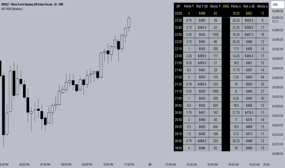
The risk table updates in real-time, showing the current stop distance, calculated contract size, and resulting risk in dollars for both upward and downward directions.
Benefit: Traders always maintain a fixed dollar risk, regardless of intraday price movement, while using HTF structure as the anchor for accurate and consistent position sizing.
1. Higher Timeframe Anchor
Always uses the last fully closed candle from the selected higher timeframe (default: 60m).
Captures the prior HTF high and low as reference boundaries.
Lower timeframe closers (e.g., 1m, 5m, 15m bars) reference these established HTF boundaries to measure stop distances and calculate risk.
Use: Ensures all position sizing is tied to completed HTF structure, providing a consistent framework for intraday trades.
2. Risk Model Engine
Traders define maximum dollar risk per trade.
The system calculates allowable micro contracts based on stop distance (current close → HTF high/low).
Supported contracts and their point values:
MNQ (Micro Nasdaq 100): $2.00 per point
MES (Micro S&P 500): $5.00 per point
MYM (Micro Dow Jones): $0.50 per point
MGC (Micro Gold): $10.00 per point
Formula:
Contracts = Max Risk ÷ (Stop Distance × TSE:VALUE per Point)
Risk ↑: Based on distance to HTF high.
Risk ↓: Based on distance to HTF low.
Use: Provides consistent dollar risk sizing across different futures contracts and multiple intraday timeframes.
3. Risk Table Overlay
Compact, real-time on-chart table with customizable styling.
Columns:
OP: Operation time (adjusted by user’s timezone offset).
Points ↑ / ↓: Stop distances in points relative to HTF boundaries.
Risk ↑ / ↓ ($): Dollar exposure at those stops.
Micros ↑ / ↓: Allowable contract count.
Asset: Displays selected futures contract in the header.
Custom features:
Independent text/background colors per column.
Highlighted latest row for clarity.
Adjustable outline, row colors, and text size.
Use: Gives traders immediate insight into position sizing without leaving the chart.
Intended Use:
This is a risk visualization module, not a trade signal generator. Traders can use it to:
Standardize risk sizing across multiple CME micro futures.
Quickly evaluate trade setups relative to HTF structure.
Measure stop distances from lower timeframe closes while referencing HTF boundaries.
Maintain consistency in risk management regardless of the instrument traded.
Limitations & Disclaimers:
Calculations assume standard CME tick values for MNQ, MES, MYM, and MGC.
Other markets may not align with these dollar-per-point values.
This indicator does not predict direction, generate entries, or guarantee outcomes.
For educational and informational purposes only.
Trading involves risk; always use proper risk management.
Closed-source (Protected): Logic is visible on charts, but source code is hidden.
Educationalposts
Auto Hourly Deviations {Module+}Description
This indicator automatically calculates and visualizes the prior hour’s price structure and its deviation levels. By combining core reference lines (high, low, EQ, quarters, open) with dynamic deviation levels and shaded zones, it provides a framework for understanding intraday price behavior relative to the most recent hourly range.
The tool has three functional sections that work together:
Core Hourly Structure – Captures the prior hour’s high, low, EQ (50%), and quarter levels (25% and 75%), plus the current open.
Deviation Levels – Projects standardized deviation multiples (±0.33, ±0.5, ±0.66, ±1.0, ±1.33, ±1.66, ±2.0) above and below the prior hour’s range.
Shading & Anchoring – Fills zones between key deviation levels for visual emphasis, while allowing projection offsets and anchor line references for precise chart alignment.
Together, these layers give traders a structured map of price movement around hourly ranges, making it easier to track expansion, retracement, and trend continuation.
1. Core Hourly Structure
Plots the prior hour’s high and low as key reference points.
Automatically calculates EQ (midpoint), 25%, and 75% levels.
Tracks the open of the current hour for immediate orientation.
Optional anchor line marks the start of each hourly window for time alignment.
Use: Frames the “hourly box” and subdivides it for intraday structure analysis.
2. Deviation Levels
Uses the prior hour’s range as a baseline.
Projects deviation levels above and below: ±0.33, ±0.5, ±0.66, ±1.0, ±1.33, ±1.66, and ±2.0.
Each level can be individually toggled with full line/label styling.
Use: Quantifies how far price is moving relative to the last hour’s volatility — useful for spotting overextensions, retraces, and probable reaction zones.
3. Shading & Anchoring
Shaded zones between selected deviation bands (e.g., +0.33 to +0.66 or +1.33 to +1.66) highlight potential liquidity or reaction areas.
Projection offsets allow levels to extend forward into future bars for planning.
Labels and color controls make the chart highly customizable.
Use: Provides quick visual cues for potential trading ranges and deviations without clutter.
Intended Use
This is a visualization tool, not a buy/sell system. Traders can use it to:
Track how price interacts with the prior hour’s high/low.
Measure hourly expansion through deviation levels.
Spot retracements or continuation zones inside and beyond the prior hour’s range.
Limitations & Disclaimers
Levels are derived from completed hourly candles; they do not predict outcomes.
Deviations are static calculations and do not account for fundamentals or volatility shifts.
This indicator does not provide financial advice or trading signals.
For informational and educational purposes only.
Trading involves risk; always apply proper risk management.
Closed-source (Protected): Logic is accessible on charts, but the source code is hidden. A TradingView paid plan is required for protected indicators.

[MAD] Acceleration based dampened SMA projectionsThis indicator utilizes concepts of arrays inside arrays to calculate and display projections of multiple Smoothed Moving Average (SMA) lines via polylines.
This is partly an experiment as an educational post, on how to work with multidimensional arrays by using User-Defined Types
------------------
Input Controls for User Interaction:
The indicator provides several input controls, allowing users to adjust parameters like the SMA window, acceleration window, and dampening factors.
This flexibility lets users customize the behavior and appearance of the indicator to fit their analysis needs.
sma length:
Defines the length of the simple moving average (SMA).
acceleration window:
Sets the window size for calculating the acceleration of the SMA.
Input Series:
Selects the input source for calculating the SMA (typically the closing price).
Offset:
Determines the offset for the input source, affecting the positioning of the SMA. Here it´s possible to add external indicators like bollinger bands,.. in that case as double sma this sma should be very short.
(Thanks Fikira for that idea)
Startfactor dampening:
Initial dampening factor for the polynomial curve projections, influencing their starting curvature.
Growfactor dampening:
Growth rate of the dampening factor, affecting how the curvature of the projections changes over time.
Prediction length:
Sets the length of the projected polylines, extending beyond the current bar.
cleanup history:
Boolean input to control whether to clear the previous polyline projections before drawing new ones.
Key technologies used in this indicator include:
User-Defined Types (UDT) :
This indicator uses UDT to create a custom type named type_polypaths.
This type is designed to store information for each polyline, including an array of points (array), a color for the polyline, and a dampening factor.
UDTs in Pine Script enable the creation of complex data structures, which are essential for organizing and manipulating data efficiently.
type type_polypaths
array polyline_points = na
color polyline_color = na
float dampening_factor= na
Arrays and Nested Arrays:
The script heavily utilizes arrays.
For example, it uses a color array (colorpreset) to store different colors for the polyline.
Moreover, an array of type_polypaths (polypaths) is used, which is an array consisting of user-defined types. Each element of this array contains another array (polyline_points), demonstrating nested array usage.
This structure is essential for handling multiple polylines, each with its set of points and attributes.
var type_polypaths polypaths = array.new()
Polyline Creation and Manipulation:
The core visual aspect of the indicator is the creation of polylines.
Polyline points are calculated based on a dampened polynomial curve, which is influenced by the SMA's slope and acceleration.
Filling initial dampening data
array_size = 9
middle_index = math.floor(array_size / 2)
for i = 0 to array_size - 1
damp_factor = f_calculate_damp_factor(i, middle_index, Startfactor, Growfactor)
polyline_color = colorpreset.get(i)
polypaths.push(type_polypaths.new(array.new(0, na), polyline_color, damp_factor))
The script dynamically generates these polyline points and stores them in the polyline_points array of each type_polypaths instance based on those prefilled dampening factors
if barstate.islast or cleanup == false
for damp_factor_index = 0 to polypaths.size() - 1
GET_RW = polypaths.get(damp_factor_index)
GET_RW.polyline_points.clear()
for i = 0 to predictionlength
y = f_dampened_poly_curve(bar_index + i , src_input , sma_slope , sma_acceleration , GET_RW.dampening_factor)
p = chart.point.from_index(bar_index + i - src_off, y)
GET_RW.polyline_points.push(p)
polypaths.set(damp_factor_index, GET_RW)
Polyline Drawout
The polyline is then drawn on the chart using the polyline.new() function, which uses these points and additional attributes like color and width.
for pl_s = 0 to polypaths.size() - 1
GET_RO = polypaths.get(pl_s)
polyline.new(points = GET_RO.polyline_points, line_width = 1, line_color = GET_RO.polyline_color, xloc = xloc.bar_index)
If the cleanup input is enabled, existing polylines are deleted before new ones are drawn, maintaining clarity and accuracy in the visualization.
if cleanup
for pl_delete in polyline.all
pl_delete.delete()
------------------
The mathematics
in the (ABDP) indicator primarily focuses on projecting the behavior of a Smoothed Moving Average (SMA) based on its current trend and acceleration.
SMA Calculation:
The indicator computes a simple moving average (SMA) over a specified window (sma_window). This SMA serves as the baseline for further calculations.
Slope and Acceleration Analysis:
It calculates the slope of the SMA by subtracting the current SMA value from its previous value. Additionally, it computes the SMA's acceleration by evaluating the sum of differences between consecutive SMA values over an acceleration window (acceleration_window). This acceleration represents the rate of change of the SMA's slope.
sma_slope = src_input - src_input
sma_acceleration = sma_acceleration_sum_calc(src_input, acceleration_window) / acceleration_window
sma_acceleration_sum_calc(src, window) =>
sum = 0.0
for i = 0 to window - 1
if not na(src )
sum := sum + src - 2 * src + src
sum
Dampening Factors:
Custom dampening factors for each polyline, which are based on the user-defined starting and growth factors (Startfactor, Growfactor).
These factors adjust the curvature of the projected polylines, simulating various future scenarios of SMA movement.
f_calculate_damp_factor(index, middle, start_factor, growth_factor) =>
start_factor + (index - middle) * growth_factor
Polynomial Curve Projection:
Using the SMA value, its slope, acceleration, and dampening factors, the script calculates points for polynomial curves. These curves represent potential future paths of the SMA, factoring in its current direction and rate of change.
f_dampened_poly_curve(index, initial_value, initial_slope, acceleration, damp_factor) =>
delta = index - bar_index
initial_value + initial_slope * delta + 0.5 * damp_factor * acceleration * delta * delta
damp_factor = f_calculate_damp_factor(i, middle_index, Startfactor, Growfactor)
Have fun trading :-)

Selected Dates Filter by @zeusbottradingWe are presenting you feature for strategies in Pine Script.
This function/pine script is about NOT opening trades on selected days. Real usage is for bank holidays or volatile days (PPI, CPI, Interest Rates etc.) in United States and United Kingdom from 2020 to 2030 (10 years of dates of bank holidays in mentioned countries above). Strategy is simple - SMA crossover of two lengts 14 and 28 with close source.
In pine script you can see we picked US and GB bank holidays. If you add this into your strategy, your bot will not open trades on those days. You must make it a rule or a condition. We use it as a rule in opening long/short trades.
You can also add some of your prefered dates, here is just example of our idea. If you want to add your preffered days you can find them on any site like forexfactory, myfxbook and so on. But don’t forget to add function “time_tradingday ! = YourChoosedDate” as it is writen lower in the pine script.
Sometimes the date is substituted for a different day, because the day of the holiday is on Saturday or Sunday.
Made with ❤️ for this community.
If you have any questions or suggestions, let us know.
The script is for informational and educational purposes only. Use of the script does not constitutes professional and/or financial advice. You alone the sole responsibility of evaluating the script output and risks associated with the use of the script. In exchange for using the script, you agree not to hold zeusbottrading TradingView user liable for any possible claim for damages arising from any decision you make based on use of the script.

Short Swing Bearish MACD Cross (By Coinrule)This strategy is oriented towards shorting during downside moves, whilst ensuring the asset is trading in a higher timeframe downtrend, and exiting after further downside.
This script can work well on coins you are planning to hodl for long-term and works especially well whilst using an automated bot that can execute your trades for you. It allows you to hedge your investment by allocating a % of your coins to trade with, whilst not risking your entire holding. This mitigates unrealised losses from hodling as it provides additional cash from the profits made. You can then choose to hodl this cash, or use it to reinvest when the market reaches attractive buying levels. Alternatively, you can use this when trading contracts on futures markets where there is no need to already own the underlying asset prior to shorting it.
ENTRY
This script utilises the MACD indicator accompanied by the Exponential Moving Average (EMA) 450 to enter trades. The MACD is a trend following momentum indicator and provides identification of short-term trend direction. In this variation it utilises the 11-period as the fast and 26-period as the slow length EMAs, with signal smoothing set at 9.
The EMA 450 is used as additional confirmation to prevent the script from shorting when price is above this long-term moving average. Once price is above the EMA 450 the script will not open any shorts - preventing the rule from attempting to short uptrends. Due to this, this strategy is ideal for setting and forgetting.
The script will enter trades based on two conditions:
1) When the MACD signals a bearish cross. This occurs when the EMA 11 crosses below the EMA 26 within the MACD signalling the start of a potential downtrend.
2) Price has closed below the EMA 450. Price closing below this long-term EMA signals that the asset is in a sustained downtrend. Price breaking above this could indicate a bullish strength in which shorting would not be profitable.
EXIT
This script utilises a set take-profit and stop-loss from the entry of the trade. The take profit is set at 8% and the stop loss of 4%, providing a risk reward ratio of 2. This indicates the script will be profitable if it has a win ratio greater than 33%.
Take-Profit Exit: -8% price decrease from entry price.
OR
Stop-Loss Exit: +4% price increase from entry price.
Based on backtesting results across a selection of assets, the 45-minute and 1-hour timeframes are the best for this strategy.
The strategy assumes each order is using 30% of the available coins to make the results more realistic and to simulate you only ran this strategy on 30% of your holdings. A trading fee of 0.1% is also taken into account and is aligned to the base fee applied on Binance.
The backtesting data was recorded from December 1st 2021, just as the market was beginning its downtrend. We therefore recommend analysing the market conditions prior to utilising this strategy as it operates best on weak coins during downtrends and bearish conditions, however the EMA 450 condition should mitigate entries during bullish market conditions.

BEST Strategy Template w/ Custom SL/TP Size - EducationalHello traders
I'm getting this question at least once per week: "how to define a custom exit quantity for my stop loss and a different one for my take profit"
Instead of answering every day the same question in my DMs, I've decided to publish an educational strategy template script using this
Features
- Select to use or not the SL and/or TP
- Define how many pips/USD the SL/TP should be set at from the entry
- Define what quantity percentage you want to close at SL and/or at TP (lines 301 to 320 in the code)
- Classical custom trailing stop where the SL is moved to breakeven once the TP is hit
- Get real-time backtesting stats based on the options you've selected
Update
You might not know it yet but from last week (or maybe the week before), the qty/qty_percent from the strategy.exit function refers now to the initial position size (and not the remaining position size like before)
For example:
strategy.exit("EX1", qty_percent = 50, stop = constant)
strategy.exit("EX2", qty_percent = 20, stop = constant)
What happened before
After "EX1" reaches SL levels, "EX2" exits 20% from the % of the remaining position size.
If the initial position size = 100 contracts
EX1 exits 50 contracts
EX2 exits 20% of 50 contracts = 10 contracts
What's happening now
After "EX1" reaches SL levels, "EX2" exits 20% from the % of the original position size.
If the initial position size = 100 contracts
EX1 exits 50 contracts
EX2 exits 20 (20% of 100 contracts) contracts
I think this is an improvement and I really enjoy this new behavior.
See you in a few days with another post :)
ALL THE BEST
Dave