Morning Straddle Backtest + Range Filter Morning Straddle Backtest
Purpose:
This script tests a Morning Straddle concept where a trader enters both long and short breakout orders based on the overnight range (22:00–06:00 by default).
It is designed for backtesting the effectiveness of volatility breakouts following low-volume overnight sessions.
Setup
Overnight session: 22:00–06:00 (adjustable).
At the end of the overnight session, the script automatically places:
A long stop order above the range high.
A short stop order below the range low.
Both use an ATR-based buffer for cleaner breakouts (default 5%).
When one side triggers, the opposite order is cancelled if OCO mode is active.
Adjustable Parameters
- Session - Defines the overnight hours used for the range.
- ATR Length - Number of bars used for ATR calculation.
- ATR Buffer % - Distance above/below range for entry & stop placement.
- Risk:Reward Ratio - Determines the TP distance relative to SL.
- Stop-Loss - Choose between “Behind Range” or “Mid-Range (50%)” with ATR buffer added.
- OCO - Cancels opposite order once one side triggers.
- Close All EOD - Closes all open trades at the end of day (default 22:00).
- Range Filter – Enables filtering of trades only when the overnight range size falls within a defined threshold.
-Min Range / Max Range – Define acceptable range size boundaries.
-Display Units – Select whether the filter is measured in Price Change, Pips, or Points.
- Stats Panel Settings – Toggle visibility, position (Top/Bottom Left/Right), and background opacity.
Visual
The overnight range (22:00–06:00) is highlighted on the chart with a teal background for clarity.
No lines are drawn for the high and low.
Strategy Notes
Works best on 5m or 15m charts where the overnight range can be clearly defined.
Backtests should be run over multiple months to gauge performance consistency.
Can be adapted for other markets by adjusting session times and ATR settings. For example, S&P initial balance breakout using 14:30-15:30 range time.
Stats Panel Displays
- 20-Day Range Data: Maximum, Average, and Minimum range sizes.
- Today’s Range: With automatic classification — Huge, Normal, or Small.
- Average Winning Range: Average size of the overnight range on profitable days.
- Average Losing Range: Average size of the overnight range on losing days.
- Filter Status: Displays whether the range met the filter criteria — Range OK, Skipped, or Off.
Educational

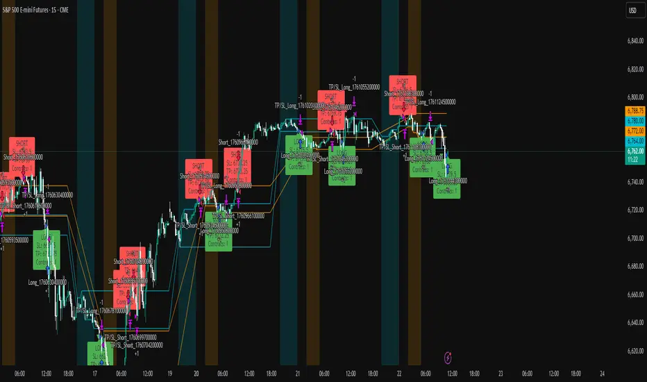
AlgoIndexOS-ES-FuturesAlgoIndexOS — ES Futures Strategy v2.0 (5-Minute RTH)
Scope (read first)
ES on 5-minute only, RTH session. The strategy operates on U.S. Regular Trading Hours (09:30–16:00 ET) using a 5-minute ES chart. It builds an Opening Session Range (OSR) from the RTH open, then runs a breakout engine when internal quality conditions are met. Exits are target-based with an intrabar touch-to-flat safety. Positions are flattened at the RTH session end by default. Alerts can post JSON to your Webhook URL for automation.
What this is
One intraday engine with four curated presets (“Stages”) tuned for distinct segments of the NY session. Stages keep the core logic consistent while applying time-of-day context and conservative governors. Single invite-only listing; not a multi-post suite.
How it trades (high-level)
Range context: Builds and locks the OSR from the opening bell; entries only arm after the range is set.
Quality gating: Trades only when internal trend/volatility/confirmation conditions align (no parameter disclosure).
Breakout execution: Signals at bar close; bracket exits manage take-profit (limit) with an intrabar “TP-touch” safety to avoid phantom fills; optional stop-loss.
Session safety: Positions flat at RTH close by default (time exit).
(No settings or thresholds are disclosed; presets encapsulate research choices.)
Stages (session templates; one engine)
A single Stage selector chooses among four presets optimized for different parts of the RTH session (morning vs mid-day; long/short focus). Internal parameters remain fixed to preserve tested behavior.
Public inputs (kept minimal)
Stage (choose your preset)
TP / SL (points) shown for transparency; effective values are governed by the selected preset to maintain consistency with research.
Optional display overlays (status line/markers) for readability.
Alerts (how to use)
Create an alert on the strategy and choose Strategy → Order fills. Use a webhook if you want automation. The payload includes the exact chart symbol so it works on ES1! or a specific ES contract:
{
"tv_symbol": "{{ticker}}",
"tv_exchange": "{{exchange}}",
"action": "buy|sell|exit",
"price": {{close}},
"time": "{{timenow}}"
}
If your receiver needs a fixed root (e.g., “ES”), map it on your server using tv_symbol for context.
Backtest & assumptions
Backtest assumptions (initial capital, commission, slippage, margin) are user-configurable in TradingView. Results on your chart reflect your settings. This script evaluates ES fills on 5-minute RTH bars; live execution will differ.
Operating notes
Use on ES only, 5-minute timeframe, RTH session.
If you run multiple Stages, use separate charts/tabs and coordinate net exposure in your own tooling if needed.
Publish with a clean chart for clarity.
Disclosures (compliance)
No investment advice. This script is for research/education and tooling only. It does not provide investment, legal, tax, or accounting advice and does not recommend any security, instrument, or strategy. Use at your own risk.
Hypothetical performance (CFTC 4.41). Hypothetical or simulated results have many limitations, and no representation is made that any account will achieve similar outcomes. Past performance is not necessarily indicative of future results.
Futures risk. Trading futures involves substantial risk of loss and is not suitable for all investors. Leverage, gaps, slippage, and connectivity can cause losses exceeding initial investment.
Backtesting limitations. Results depend on data quality, chart resolution, session filters, and user assumptions; live execution will differ.
Intellectual property. © 2025 AlgoIndex. All Rights Reserved. Redistribution, resale, or decompilation prohibited without written consent.

12M SMA Timing (HTF-safe, 100% equity)Buy when S&P500 closes above 12M moving average. Sell when it closes below it. Monthly only.

WIN1! • Crossing EMAs• (By Mesquita, v7)Moving average crossover strategy for intraday movements, especially in the continuous index (WIN1!) on the Brazilian stock exchange B³. The strategy is customizable for time windows, has a filter for trades only above the long-term average, whether only long, only short, or both, with or without stop loss.

KZ One — Scalping Training StrategyKZ One is a scalping strategy developed for M1 and M5 timeframes. It is designed to help traders study and practice short-term market behavior by using structured zones to highlight potential entry and exit areas. The strategy allows customization of Risk (USD) and Take Profit (R multiple) parameters for flexible trade management. Additional tools include ATR-based filters to skip low-volatility conditions and a Pre-Alert Lead (bars) option that notifies users ahead of possible setups. KZ One is intended for educational and analytical purposes, promoting disciplined and consistent trading practice.

💸 DCA Accumulation Strategy (USD‑Based Scaling)Buy when blue arrow appears, if the next arrow is lower than the last increase your position. This will pull your average cost down slowly over time.

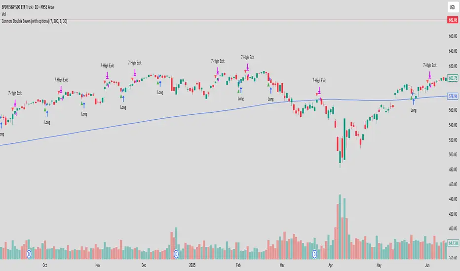
Connors Double Seven (with options)Rules (original, long-only)
Trade only when Close > 200-day SMA.
Entry: Buy when Close makes a 7-day low.
Exit: Sell when Close makes a 7-day high.
MoneyPlant-Auto Support Resistance V2.0
🧭 Overview
MoneyPlant – Auto Support Resistance is a professional-grade indicator designed to automatically detect dynamic Support and Resistance levels using real-time market structure.
It combines trend confirmation, structure analysis, and momentum logic to identify high-probability trading zones in all market conditions.
⚙️ Core Concept
This indicator uses a unique combination of classic and proprietary logic to filter only the most relevant S/R levels:
• Dynamic Support/Resistance Mapping: Detects strong reaction levels based on price structure, candle rejection points, and breakout validation.
• EMA & WMA Trend Filter: Uses a triple-moving-average model (default EMA 18, EMA 25, and WMA 7) to confirm current market bias.
• MACD Momentum Filter: Confirms trend strength and helps avoid false breakouts.
• Smart Alignment Logic: Generates signals only when structure, trend, and momentum all align in the same direction.
🧠 How It Works
1. Buy Setup:
When price breaks above a resistance level with bullish EMA/WMA alignment and positive MACD momentum → Buy Signal triggers.
2. Sell Setup:
When price breaks below a support level with bearish EMA/WMA alignment and negative MACD momentum → Sell Signal triggers.
3. Auto-Refreshing Zones:
Support and Resistance zones update dynamically as market structure evolves.
🎯 Best Use Cases
• Works effectively on Stocks, Indices, Forex, and Commodities (e.g., XAUUSD, NIFTY, BANKNIFTY ).
• Ideal for Intraday & Swing Trading (15 min – 1 hour timeframes).
• Fully compatible with TradingView alerts and automation tools.
💡 Key Features
✅ Automatic Support/Resistance detection
✅ Adaptive EMA + WMA + MACD trend logic
✅ Real-time Buy/Sell alerts
✅ Multi-timeframe compatibility
✅ Optimized for clean chart visuals
⚖️ Recommended Settings
• EMA Fast: 18
• EMA Slow: 25
• WMA Filter: 7
• MACD: Default parameters
(Users may adjust EMA/WMA settings according to their own trading style.)
🔒 How to Get Access
To get access to this invite-only script, please send me a private message on TradingView or use the link in my profile.
Once your username is added via Manage Access, you’ll be able to use the indicator.
🧾 Notes for Traders
This tool does not repaint, and it’s meant for educational and analytical purposes only.
Each license is valid for one TradingView username — no resale or redistribution is permitted.
Developed by MoneyPlant
Smart Automation for Professional Traders

Basic DCA Strategy by Wongsakon KhaisaengThe Core Principle and Philosophy Behind the Basic DCA Strategy
1. Introduction
The Basic DCA Strategy (Dollar-Cost Averaging) represents one of the most fundamental and enduring investment methodologies in the realm of systematic accumulation. The philosophy underpinning DCA is rooted not in speculation or prediction, but in disciplined participation. It assumes that the consistent act of investing a fixed amount of capital over time—regardless of short-term price volatility—can yield superior long-term outcomes through the natural smoothing effect of cost averaging.
This strategy, expressed through the Pine Script code above, formalizes the DCA concept into a fully systematic trading framework, enabling quantitative backtesting and objective evaluation of long-term accumulation efficiency.
2. Mechanism of Operation
At its technical core, the strategy executes a fixed-value buy order at every predefined interval within a specific accumulation period.
Each DCA event invests a constant “Investment Amount (USD)” irrespective of price fluctuations. When prices decline, this constant investment buys a larger quantity of the asset; when prices rise, it purchases fewer units. Over time, this behavior lowers the average cost basis of the accumulated position, effectively neutralizing short-term timing risks.
Mathematically, this is represented as:
Units Purchased = Investment Amount / Closing Price
Cost Basis = Total Invested USD / Total Units Acquired
Portfolio Value = Total Units Acquired × Current Price
The algorithm tracks cumulative investment, acquired units, and commissions dynamically, continuously recalculating key portfolio metrics such as total profit/loss (PnL), CAGR (Compound Annual Growth Rate), and maximum drawdown (peak-to-trough equity decline).
Furthermore, the script juxtaposes DCA results with a Buy & Hold benchmark, where the entire initial capital is invested at once. This comparison highlights the behavioral resilience and volatility resistance of the DCA method relative to market-timing strategies.
3. The Essence of DCA Philosophy
At its philosophical core, DCA is not a trading system, but a behavioral framework for rational capital deployment under uncertainty. It embodies the principle that time in the market often outweighs timing the market.
The DCA approach rejects the illusion of precision forecasting and embraces probabilistic humility—the recognition that even the most skilled investors cannot consistently predict short-term market fluctuations. Instead, it focuses on controlling what is controllable: the frequency, consistency, and size of investment actions.
This mindset reflects a broader principle of risk dispersion through temporal diversification. Rather than concentrating entry risk into a single price point (as in lump-sum investing), DCA spreads exposure across multiple time intervals, thereby converting volatility into opportunity.
In essence, volatility—often perceived as risk—is reframed as a mechanism for mean reversion advantage. The strategy thrives precisely because markets oscillate; each fluctuation provides a chance to accumulate at varied price levels, improving the weighted-average entry over time.
4. Long-Term Rationality Over Short-Term Emotion
DCA’s endurance stems from its ability to neutralize emotional biases inherent in human decision-making. Investors tend to overreact to market euphoria or panic—buying high out of greed and selling low out of fear. By automating purchases through predefined intervals, the DCA model enforces mechanical discipline, detaching decision-making from sentiment.
This transforms investing from an emotional endeavor into a systematic, algorithmic routine governed by rules rather than reactions. In doing so, DCA serves not only as a financial model but also as a psychological safeguard—aligning investor behavior with long-term compounding logic rather than short-term speculation.
5. Comparative Insight: DCA vs. Buy & Hold
While both DCA and Buy & Hold share a long-term investment horizon, they diverge in their treatment of entry timing. The Buy & Hold model assumes full deployment of capital at the beginning, maximizing exposure to growth but also to volatility. Conversely, DCA smooths the entry curve, trading off short-term returns for long-term stability and improved average entry price.
In environments characterized by volatility and cyclical corrections, DCA tends to outperform in terms of risk-adjusted returns, lower drawdowns, and improved investor adherence—since it reduces the psychological pain of entering at local peaks.
6. Conclusion
The Basic DCA Strategy exemplifies the synthesis of mathematical rigor and behavioral discipline. Its algorithmic construction in Pine Script transforms a classical investment philosophy into a quantifiable, testable, and transparent framework.
By automating fixed-amount purchases across time, the system operationalizes the central axiom of DCA: consistency over conviction. It is not concerned with predicting future prices but with ensuring persistent participation—trusting that the market’s upward bias and the power of compounding will reward patience more than precision.
Ultimately, DCA embodies the timeless principle that successful investing is less about forecasting markets, and more about designing behavior that can endure them.

Nifty Intraday 9:30- 3 Min Candle By Trade Prime Algo.Nifty Intraday 9:30 – 3 Min Candle Strategy by Trade Prime Algo
This strategy is designed to help traders identify intraday long entries, stop-loss, and multi-target levels on the Nifty Spot / Nifty Futures based on the first 3-minute candle breakout after 9:30 AM.
It automates trade detection, entry marking, target plotting, and trailing stop-loss logic, allowing traders to visualize complete trade flow with clarity and precision.
The system offers:
✅ Auto identification of long entries based on candle breakout logic
✅ Configurable stop-loss, trailing SL, and four partial profit targets
✅ Dynamic plotting of entry, TSL, and targets on chart
✅ Custom alert messages for each event (Entry, TP1–TP4, SL, Close)
✅ Adjustable time session and test periods for backtesting
⚙️ How to Use
1️⃣ Set your desired start time (default: 9:15–9:30 AM).
2️⃣ Choose your stop-loss type — percentage or points.
3️⃣ Adjust target levels (TP1–TP4) and trailing SL settings as per your risk appetite.
4️⃣ Use this strategy for educational backtesting and research only — not for live trading signals.
5️⃣ The tool can be combined with price action zones or higher-timeframe analysis for best results.
⚠️ Disclaimer (SEBI & Risk Disclosure)
This strategy is developed strictly for educational and research purposes.
The creator of this script and Trade Prime Algo are not SEBI-registered advisors.
This tool does not guarantee any specific profit or performance.
Trading involves risk; users may incur partial or total capital loss.
All decisions taken using this indicator or strategy are solely at the user’s discretion and risk.
The creator assumes no liability for profit, loss, or any consequences arising from the use of this script.
Always perform your own due diligence and trade responsibly.

15-min ORB — NY 9:30 (SPX) 10232025This strategy trades the New York session opening range breakout (ORB) using a 15-minute window that starts at 9:30 AM New York time (6:30 AM PDT). It identifies the high and low formed during the first ORB period (default 15 minutes), then looks for breakouts above or below that range within the next 100 minutes of the session.

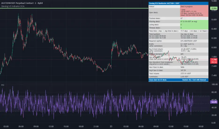
Zendog V3 Indicator DCAThis strategy is same as Zendog v3 but edited to be backtest compatible for SO additions through indicator
for Longs
Safety order type = External indicator
External indicator = RSI 30/70 : Long Trigger
Safety Order Value = 1
for Shorts
Safety order type = External indicator
External indicator = RSI 30/70 : Short Trigger
Safety Order Value = 2
Cava Signals Backtesting v2Cava Signals Backtesting Strategy v2 (BTC)
This Pine Script strategy is designed for backtesting trading signals on BTC, built upon the Cava Signals v2 framework. It integrates multiple technical indicators to identify potential buy and sell opportunities, incorporating volume analysis, momentum, and trend-following mechanisms. The strategy supports customizable parameters for trade entry, exit, take-profit, stop-loss, and DCA (Dollar-Cost Averaging) logic, optimized for BTC trading. Ideal for traders looking to test and refine their approach in a backtesting environment, this script offers flexibility to adapt to various market conditions while focusing on disciplined trade management. Always backtest thoroughly and validate performance before live use.

Enhanced OB Retest Strategy v7.0The OB Retest Strategy is a full Order Block retest trading system that detects, plots, and trades OB zones across multiple timeframes. It uses structure breaks, retrace depth, and ATR filters to identify strong reversal or continuation setups.
⸻
⚙️ Core Features
• Multi-timeframe OB detection using break-of-structure (BOS) logic
• Automatic zone creation for bullish and bearish order blocks
• Smart merging of overlapping OB zones
• Dynamic flip-zone logic that turns invalidated OBs into new zones
• Wick zone detection for high-precision entries
• ATR-based trailing stop and optional breakeven
• Adjustable retrace depth, breakout %, and ATR filters
• Built-in performance table showing PnL, win rate, and total trades
• Fully backtestable with date range and commission control
⸻
🧠 Logic Summary
1. Detects a BOS on the higher timeframe.
2. Identifies the last opposing candle as the valid OB.
3. Validates the OB based on ATR size and breakout strength.
4. Waits for price to retest the zone to a set depth.
5. Executes trades and manages exits using trailing stop or breakeven.
6. Flips invalidated zones automatically.
⸻
💡 Usage Tips
• Best used on 1H to 4H charts for swing setups.
• Tune ATR and breakout thresholds for your market’s volatility.
• Combine with higher-timeframe bias or liquidity levels for better accuracy.
⸻
⚠️ Notes
• For educational and testing purposes only.
• Backtested results do not predict future performance.
• Always test before live use.

ICT Liquidity Sweep Asia/London 1 Trade per High & Low🧠 ICT Liquidity Sweep Asia/London — 1 Trade per High & Low
This strategy is inspired by the ICT (Inner Circle Trader) concepts of liquidity sweeps and market structure, focusing on the Asia and London sessions.
It automatically identifies liquidity grabs (sweeps) above or below key session highs/lows and enters trades with a fixed risk/reward ratio (RR).
----------------------------------------------------------------------------------
----------------------------------------------------------------------------------
⚙️ Core Logic
-Asia Session: 8:00 PM – 11:59 PM (New York time)
-London Session: 2:00 AM – 5:00 AM (New York time)
-The script marks the Asia High/Low and London High/Low ranges for each day.
-When the market sweeps above a session high → potential Short setup
-When the market sweeps below a session low → potential Long setup
-A trade is triggered when the confirmation candle closes in the opposite direction of the sweep (bearish after a high sweep, bullish after a low sweep).
-Only one trade per sweep type (1 per High, 1 per Low) is allowed per session.
----------------------------------------------------------------------------------
----------------------------------------------------------------------------------
📈 Risk Management
-Configurable Risk/Reward Target (default = 2:1)
-Configurable Position Size (number of contracts)
-Each trade uses a fixed Stop Loss (beyond the wick of the sweep) and a Take Profit calculated from the RR setting.
-All trades are automatically logged in the Strategy Tester with performance metrics.
----------------------------------------------------------------------------------
----------------------------------------------------------------------------------
💡 Features
✅ Visual session highlighting (Asia = Aqua, London = Orange)
✅ Automatic liquidity line plotting (session highs/lows)
✅ Entry & exit labels (optional visual display)
✅ Customizable RR and contract size
✅ Works on any instrument (ideal for indices, futures, or forex)
✅ Compatible with all timeframes (optimized for 1M–15M)
----------------------------------------------------------------------------------
----------------------------------------------------------------------------------
⚠️ Notes
-Best used on New York time-based charts.
-Designed for educational and backtesting purposes — not financial advice.
-Use as a foundation for further optimization (e.g., SMT confirmation, FVG filter, or time-based restrictions).
----------------------------------------------------------------------------------
----------------------------------------------------------------------------------
🧩 Recommended Use
Pair this with:
-ICT’s concepts like CISD (Change in State of Delivery) and FVGs (Fair Value Gaps)
-Higher timeframe liquidity maps
-Session bias or daily narrative filters
----------------------------------------------------------------------------------
----------------------------------------------------------------------------------
Author: jygirouard
Strategy Version: 1.3
Type: ICT Liquidity Sweep Automation
Timezone: America/New_York
4-Hour Range Scalping [v6.3]User Guide: 4-Hour Range Scalping Strategy
Hello! Here is the guide for the Pine Script strategy. Please read it carefully to get the best results.
📈 This script automates the "4-Hour Range Scalping Strategy" from the video.
The main idea is that the first four hours of a major trading day (like New York) set up a "trap zone." The strategy waits for the price to break out of this zone and then fail, giving us a signal that the breakout was false and the price is likely to reverse.
Here’s the simple logic:
Define the Range: It precisely calculates the highest high and lowest low during the first four hours of the selected trading session (e.g., 00:00 to 04:00 New York Time).
Wait for a Breakout: It then monitors the 5-minute chart for a price breakout where a candle fully closes outside of this established range.
Identify the Reversal: The trade trigger occurs when the price fails to continue its breakout and a subsequent 5-minute candle closes back inside the range. This signals a potential reversal or "failed breakout."
Execute the Trade:
]A Short (Sell) trade is triggered after a failed breakout above the range high.
A Long (Buy) trade is triggered after a failed breakout below the range low.
Manage the Risk: The Stop Loss is automatically placed at the peak (for shorts) or trough (for longs) of the breakout move, and the Take Profit is set to a default 2:1 Risk/Reward Ratio.
How to Use the Script (Step-by-Step) ⚙️
Follow these instructions to get it running perfectly.
1. Set Your Chart Timeframe This is the most important step. The strategy is designed to run on a 5-minute (5m) chart. Open your TradingView chart and make sure the timeframe is set to "5m".
2. Add the Script to Your Chart Open the Pine Editor tab at the bottom of TradingView, paste the entire script, and click the "Add to chart" button.
3. Configure the Settings On your chart, find the strategy's name (e.g., "4-Hour Range Scalping ") and click the gear icon ⚙️ to open its settings.
Trading Session: Choose the session for the range. New York is the default and the one from the video.
Risk/Reward Ratio: The default is 2.0, meaning your potential profit is twice your potential loss. You can adjust this to test other targets.
Backtesting Period: To see how the strategy performed on all historical data, go to the "Strategy Tester" panel, click its own gear icon ⚙️, and uncheck the boxes for "Start Date" and "End Date."
4. Understand the Visuals on Your Chart
Blue Background Area: This is the 4-hour calculation window. The script is identifying the day's high and low during this time. No trades will ever happen here.
Red Line (Range High): The highest price of the 4-hour window. This is the upper boundary of the "trap zone."
Green Line (Range Low): The lowest price of the 4-hour window. This is the lower boundary.
Green Triangle (▲): Shows where a Long (Buy) trade was entered.
Red Triangle (▼): Shows where a Short (Sell) trade was entered.
A Very Important Note on Timezones 🕒
This is critical for you in the Philippines (PHT).
The script is based on the New York session, which is 12 hours behind you. Your TradingView chart will still show your local time, but the script works on NY time in the background.
The New York "day" begins at 12:00 PM (Noon) your time.
The script's blue calculation window will be from 12:00 PM to 4:00 PM your local time.
The red and green range lines will appear on your chart only after 4:00 PM your time.
So, if you look at your chart in the morning or early afternoon, you will not see today's range yet. This is normal! The script is just waiting for the New York session to start.
How to Set Up Trade Alerts 🔔
You can have TradingView send you a notification whenever the script enters a trade.
Click the "Alert" button (looks like a clock) in the right-hand toolbar of TradingView.
In the "Condition" dropdown, select the name of the script (e.g., "4-Hour Range Scalping...").
You will then see two options: "Long Signal" and "Short Signal".
Select one (e.g., "Long Signal") and configure how you want to be notified (e.g., "Notify on app").
Click "Create". Repeat the process to create an alert for the other signal.
⚠️ Important Disclosure
For Educational and Research Purposes Only.
This script and all accompanying information are provided for educational and research purposes only. The strategy demonstrated is a technical concept and should not be misconstrued as financial, investment, legal, or tax advice.
Trading financial markets involves substantial risk and is not suitable for every investor. There is a possibility that you could sustain a loss of some or all of your initial investment. Therefore, you should not invest money that you cannot afford to lose.
Past performance is not indicative of future results. The backtesting results shown by this script are historical and do not guarantee future performance. Market conditions are constantly changing.
By using this script, you acknowledge that you are solely responsible for any and all trading decisions you make. You should conduct your own thorough research and, if necessary, seek advice from an independent financial advisor before making any investment decisions. The creators of this script assume no liability for any of your trading results.

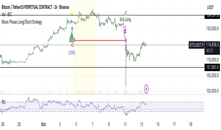
Moon Phases Long/Short StrategyThis is an experiment of Moon Phases, likely buy when full moon and sell when new moon with few changes, like it would buy a day ahead or sometimes sell a day post these events, with Stop loss and take profits, 50% profitable so sounds good to me
Long only good for bitcoin gold, both modes(L+S) better for stocks and alt coins
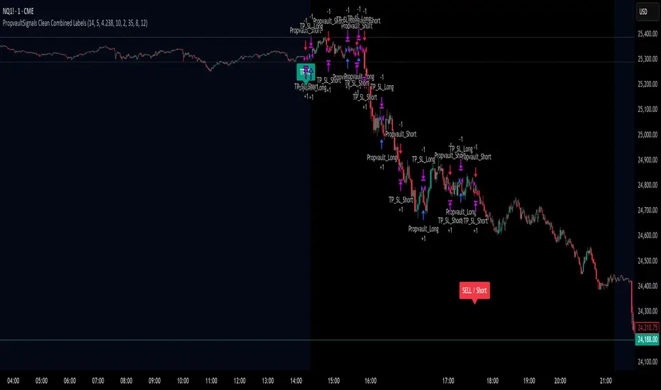
PropvaultSignals Clean Combined Labels Best Tested 91%PropvaultSignals Clean Single Label with best session
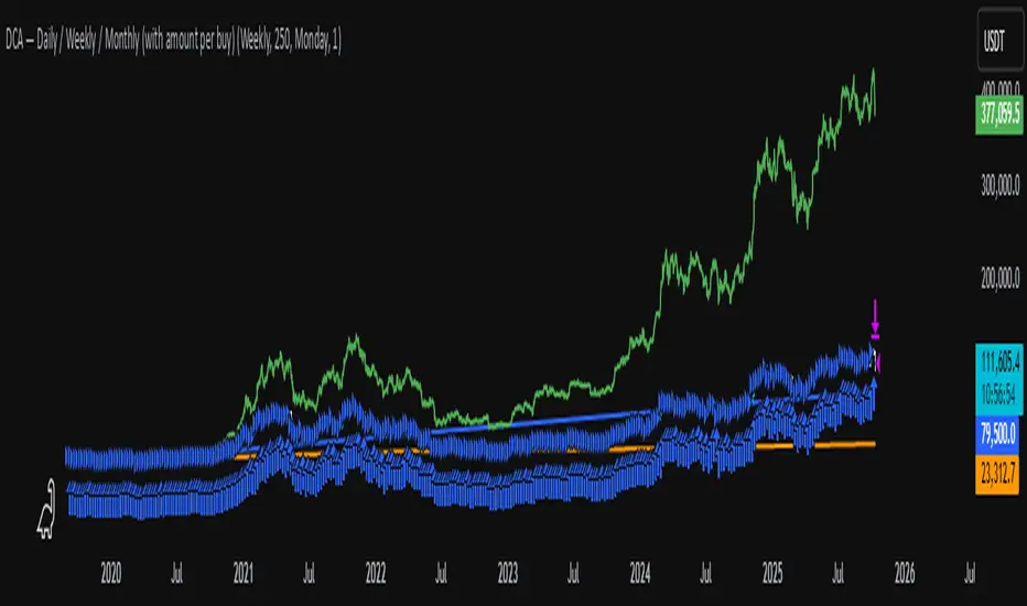
DCA Test Daily / Weekly / Monthly1.Input daily, weekly or monthly preferance of DCA
2.Select how much to DCA
3.Use the slider on the indicator down to select from where to DCA
Important: Don't use a higher timeframe chart than the desired DCA frequency, or all the DCA buys won't get executed.
DCA with the Money Supply Index DCA with the Money Supply Index (MSI) by zdmre
This strategy is based on the Money Supply Index (MSI) by zdmre and enhances it with two functional options for users: a DCA (Dollar-Cost Averaging) approach and a signal-based buy/sell mode. It’s designed to help traders and investors make data-driven, disciplined entry decisions based on monetary supply trends.
🧠 Concept Overview
The Money Supply Index (MSI) provides insight into how liquidity (money supply) influences market movements. This strategy builds upon that foundation by allowing users to either:
Accumulate positions over time using DCA, based on favorable MSI conditions.
Execute a single buy and sell trade, optimized for bull market conditions.
⚙️ Inputs Explained
General Parameters
Start Bar Index / Stop Bar Index
Defines the range of bars (historical data) for backtesting or strategy visualization.
Long DCA
Activates the DCA mode. If unchecked, the strategy operates in single-entry/single-exit signal mode.
Trading Signal
Enables signal-based entries and exits when the MSI reaches predefined thresholds.
DCA Parameters
Entry Value
The MSI value that triggers a DCA buy event. When the MSI crosses below this value, the strategy considers it a favorable moment to deploy the saved capital.
Saved Amount
The amount of money set aside regularly (e.g., monthly) for investment. This simulates the DCA effect by accumulating capital and deploying it when conditions are optimal.
Data Inputs
Money Supply
The data source for the Money Supply Index (default: ECONOMICS:USM2).
Relational Symbol
The market instrument to compare against the money supply (default: NASDAQ_DLY:NDX). This allows the strategy to measure liquidity impact on a specific market.
Chart Display Options
You can toggle these metrics on the chart for better visualization:
Entry Price (green) – The price level of executed buys.
Cash Balance (yellow) – Remaining uninvested capital.
Invested Capital (red) – Total amount currently invested.
Current Value (blue) – The current valuation of the investment.
Profit (purple) – The total realized and unrealized profit.
Trades on Chart / Signal Labels / Quantity – Enables trade markers, signal text, and position size visualization.
📈 How the Strategy Works
1️⃣ DCA Mode
In DCA mode, the strategy simulates periodic savings and only invests when the MSI indicates favorable liquidity conditions (based on the Entry Value).
This approach aims to achieve the best possible average entry price over time — a powerful strategy for long-term investors seeking stable accumulation with reduced emotional bias.
2️⃣ Signal-Based Mode
In signal mode (with DCA disabled), the strategy performs one buy and one sell trade based on MSI turning points.
It’s most effective during bull markets, where liquidity expansion supports upward momentum.
This mode helps identify high-probability entry and exit zones rather than averaging in continuously.
💡 Additional Notes
This strategy includes helpful metrics to monitor your personal investment performance — showing invested capital, cash reserves, and profit in real-time.
The goal is to combine macroeconomic insight (money supply) with disciplined execution and capital management.
⚠️ Disclaimer
This strategy is for educational and research purposes only. It does not constitute financial advice. Always conduct your own analysis before making investment decisions.

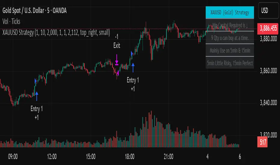
Golden StrategyTitle: XAUUSD (Gold) Smart Entry Strategy with Dynamic Scaling
Description:
This is a precision-based entry strategy for XAUUSD (Gold), optimized for lower timeframes like the 5-minute and 15-minute charts. It uses a custom logic engine to detect potential reversals and applies dynamic scaling (pyramiding) to build positions strategically based on price behavior.
🔍 Key Features:
✅ Smart entry logic for trend shifts
✅ Configurable position scaling up to 7 level
✅ Built-in capital efficiency for smaller accounts
✅ Backtest window control for historical testing
✅ Compact on-screen table for user guidance
Timeframes Recommended:
🔸 15-minute: Best balance of risk and consistency
🔸 5-minute: More frequent signals, slightly higher risk
⚠️ Important Disclaimer
This script is for educational and informational purposes only. It is not financial advice or a signal service. Trading carries risk, and past performance does not guarantee future results. Use at your own discretion and always manage risk appropriately.
Diabolos Long What the strategy tries to do
It looks for RSI dips into oversold, then waits for RSI to recover above a chosen level before placing a limit buy slightly below the current price. If the limit doesn’t fill within a few bars, it cancels it. Once in a trade, it sets a fixed take-profit and stop-loss. It can pyramid up to 3 entries.
Step-by-step
1) Inputs you control
RSI Length (rsiLen), Oversold level (rsiOS), and a re-entry threshold (rsiEntryLevel) you want RSI to reach after oversold.
Entry offset % (entryOffset): how far below the current close to place your limit buy.
Cancel after N bars (cancelAfterBars): if still not filled after this many bars, the limit order is canceled.
Risk & compounding knobs: initialRisk (% of equity for first order), compoundRate (% to artificially grow the equity base after each signal), plus fixed TP% and SL%.
2) RSI logic (arming the setup)
It calculates rsi = ta.rsi(close, rsiLen).
If RSI falls below rsiOS, it sets a flag inOversold := true (this “arms” the next potential long).
A long signal (longCondition) happens only when:
inOversold is true (we were oversold),
RSI comes back above rsiOS,
and RSI is at least rsiEntryLevel.
So: dip into OS → recover above OS and to your threshold → signal fires.
3) Placing the entry order
When longCondition is true:
It computes a limit price: close * (1 - entryOffset/100) (i.e., below the current bar’s close).
It sizes the order as positionRisk / close, where:
positionRisk starts as accountEquity * (initialRisk/100).
accountEquity was set once at script start to strategy.equity.
It places a limit long: strategy.order("Long Entry", strategy.long, qty=..., limit=limitPrice).
It then resets inOversold := false (disarms until RSI goes oversold again).
It remembers the bar index (orderBarIndex := bar_index) so it can cancel later if unfilled.
Important nuance about “compounding” here
After signaling, it does:
compoundedEquity := compoundedEquity * (1 + compoundRate/100)
positionRisk := compoundedEquity * (initialRisk/100)
This means your future order sizes grow by a fixed compound rate every time a signal occurs, regardless of whether previous trades won or lost. It’s not tied to actual PnL; it’s an artificial growth curve. Also, accountEquity was captured only once at start, so it doesn’t automatically track live equity changes.
4) Auto-cancel the limit if it doesn’t fill
On each bar, if bar_index - orderBarIndex >= cancelAfterBars, it does strategy.cancel("Long Entry") and clears orderBarIndex.
If the order already filled, cancel does nothing (there’s nothing pending with that id).
Behavioral consequence: Because you set inOversold := false at signal time (not on fill), if a limit order never fills and later gets canceled, the strategy will not fire a new entry until RSI goes below oversold again to re-arm.
5) Managing the open position
If strategy.position_size > 0, it reads the avg entry price, then sets:
takeProfitPrice = avgEntryPrice * (1 + exitGainPercentage/100)
stopLossPrice = avgEntryPrice * (1 - stopLossPercentage/100)
It places a combined exit:
strategy.exit("TP / SL", from_entry="Long Entry", limit=takeProfitPrice, stop=stopLossPrice)
With pyramiding=3, multiple fills can stack into one net long position. Using the same from_entry id ties the TP/SL to that logical entry group (not per-layer). That’s OK in TradingView (it will manage TP/SL for the position), but you don’t get per-layer TP/SL.
6) Visuals & alerts
It plots a green triangle under the bar when the long signal condition occurs.
It exposes an alert you can hook to: “Покупка при достижении уровня”.
A quick example timeline
RSI drops below rsiOS → inOversold = true (armed).
RSI rises back above rsiOS and reaches rsiEntryLevel → signal.
Strategy places a limit buy a bit below current price.
4a) If price dips to fill within cancelAfterBars, you’re long. TP/SL are set as fixed % from avg entry.
4b) If price doesn’t dip enough, after N bars the limit is canceled. The system won’t re-try until RSI becomes oversold again.
Key quirks to be aware of
Risk sizing isn’t PnL-aware. accountEquity is frozen at start, and compoundedEquity grows on every signal, not on wins. So size doesn’t reflect real equity changes unless you rewrite it to use strategy.equity each time and (optionally) size by stop distance.
Disarm on signal, not on fill. If a limit order goes stale and is canceled, the system won’t try again unless RSI re-enters oversold. That’s intentional but can reduce fills.
Single TP/SL id for pyramiding. Works, but you can’t manage each add-on with different exits.

Zero Lag + Momentum Bias StrategyZero Lag + Momentum Bias Strategy (MTF + Strong MBI + R:R + Partial TP + Alerts)
