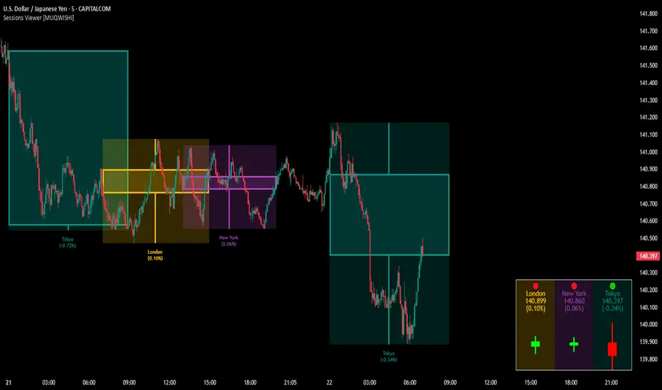
CVD - Cumulative Volume Delta (Chart)█ OVERVIEW
This indicator displays cumulative volume delta (CVD) as an on-chart oscillator. It uses intrabar analysis to obtain more precise volume delta information compared to methods that only use the chart's timeframe.
The core concepts in this script come from our first CVD indicator , which displays CVD values as plot candles in a separate indicator pane. In this script, CVD values are scaled according to price ranges and represented on the main chart pane.
█ CONCEPTS
Bar polarity
Bar polarity refers to the position of the close price relative to the open price. In other words, bar polarity is the direction of price change.
Intrabars
Intrabars are chart bars at a lower timeframe than the chart's. Each 1H chart bar of a 24x7 market will, for example, usually contain 60 bars at the lower timeframe of 1min, provided there was market activity during each minute of the hour. Mining information from intrabars can be useful in that it offers traders visibility on the activity inside a chart bar.
Lower timeframes (LTFs)
A lower timeframe is a timeframe that is smaller than the chart's timeframe. This script utilizes a LTF to analyze intrabars, or price changes within a chart bar. The lower the LTF, the more intrabars are analyzed, but the less chart bars can display information due to the limited number of intrabars that can be analyzed.
Volume delta
Volume delta is a measure that separates volume into "up" and "down" parts, then takes the difference to estimate the net demand for the asset. This approach gives traders a more detailed insight when analyzing volume and market sentiment. There are several methods for determining whether an asset's volume belongs in the "up" or "down" category. Some indicators, such as On Balance Volume and the Klinger Oscillator , use the change in price between bars to assign volume values to the appropriate category. Others, such as Chaikin Money Flow , make assumptions based on open, high, low, and close prices. The most accurate method involves using tick data to determine whether each transaction occurred at the bid or ask price and assigning the volume value to the appropriate category accordingly. However, this method requires a large amount of data on historical bars, which can limit the historical depth of charts and the number of symbols for which tick data is available.
In the context where historical tick data is not yet available on TradingView, intrabar analysis is the most precise technique to calculate volume delta on historical bars on our charts. This indicator uses intrabar analysis to achieve a compromise between simplicity and accuracy in calculating volume delta on historical bars. Our Volume Profile indicators use it as well. Other volume delta indicators in our Community Scripts , such as the Realtime 5D Profile , use real-time chart updates to achieve more precise volume delta calculations. However, these indicators aren't suitable for analyzing historical bars since they only work for real-time analysis.
This is the logic we use to assign intrabar volume to the "up" or "down" category:
• If the intrabar's open and close values are different, their relative position is used.
• If the intrabar's open and close values are the same, the difference between the intrabar's close and the previous intrabar's close is used.
• As a last resort, when there is no movement during an intrabar and it closes at the same price as the previous intrabar, the last known polarity is used.
Once all intrabars comprising a chart bar are analyzed, we calculate the net difference between "up" and "down" intrabar volume to produce the volume delta for the chart bar.
█ FEATURES
CVD resets
The "cumulative" part of the indicator's name stems from the fact that calculations accumulate during a period of time. By periodically resetting the volume delta accumulation, we can analyze the progression of volume delta across manageable chunks, which is often more useful than looking at volume delta accumulated from the beginning of a chart's history.
You can configure the reset period using the "CVD Resets" input, which offers the following selections:
• None : Calculations do not reset.
• On a fixed higher timeframe : Calculations reset on the higher timeframe you select in the "Fixed higher timeframe" field.
• At a fixed time that you specify.
• At the beginning of the regular session .
• On trend changes : Calculations reset on the direction change of either the Aroon indicator, Parabolic SAR , or Supertrend .
• On a stepped higher timeframe : Calculations reset on a higher timeframe automatically stepped using the chart's timeframe and following these rules:
Chart TF HTF
< 1min 1H
< 3H 1D
<= 12H 1W
< 1W 1M
>= 1W 1Y
Specifying intrabar precision
Ten options are included in the script to control the number of intrabars used per chart bar for calculations. The greater the number of intrabars per chart bar, the fewer chart bars can be analyzed.
The first five options allow users to specify the approximate amount of chart bars to be covered:
• Least Precise (Most chart bars) : Covers all chart bars by dividing the current timeframe by four.
This ensures the highest level of intrabar precision while achieving complete coverage for the dataset.
• Less Precise (Some chart bars) & More Precise (Less chart bars) : These options calculate a stepped LTF in relation to the current chart's timeframe.
• Very precise (2min intrabars) : Uses the second highest quantity of intrabars possible with the 2min LTF.
• Most precise (1min intrabars) : Uses the maximum quantity of intrabars possible with the 1min LTF.
The stepped lower timeframe for "Less Precise" and "More Precise" options is calculated from the current chart's timeframe as follows:
Chart Timeframe Lower Timeframe
Less Precise More Precise
< 1hr 1min 1min
< 1D 15min 1min
< 1W 2hr 30min
> 1W 1D 60min
The last five options allow users to specify an approximate fixed number of intrabars to analyze per chart bar. The available choices are 12, 24, 50, 100, and 250. The script will calculate the LTF which most closely approximates the specified number of intrabars per chart bar. Keep in mind that due to factors such as the length of a ticker's sessions and rounding of the LTF, it is not always possible to produce the exact number specified. However, the script will do its best to get as close to the value as possible.
As there is a limit to the number of intrabars that can be analyzed by a script, a tradeoff occurs between the number of intrabars analyzed per chart bar and the chart bars for which calculations are possible.
Display
This script displays raw or cumulative volume delta values on the chart as either line or histogram oscillator zones scaled according to the price chart, allowing traders to visualize volume activity on each bar or cumulatively over time. The indicator's background shows where CVD resets occur, demarcating the beginning of new zones. The vertical axis of each oscillator zone is scaled relative to the one with the highest price range, and the oscillator values are scaled relative to the highest volume delta. A vertical offset is applied to each oscillator zone so that the highest oscillator value aligns with the lowest price. This method ensures an accurate, intuitive visual comparison of volume activity within zones, as the scale is consistent across the chart, and oscillator values sit below prices. The vertical scale of oscillator zones can be adjusted using the "Zone Height" input in the script settings.
This script displays labels at the highest and lowest oscillator values in each zone, which can be enabled using the "Hi/Lo Labels" input in the "Visuals" section of the script settings. Additionally, the oscillator's value on a chart bar is displayed as a tooltip when a user hovers over the bar, which can be enabled using the "Value Tooltips" input.
Divergences occur when the polarity of volume delta does not match that of the chart bar. The script displays divergences as bar colors and background colors that can be enabled using the "Color bars on divergences" and "Color background on divergences" inputs.
An information box in the lower-left corner of the indicator displays the HTF used for resets, the LTF used for intrabars, the average quantity of intrabars per chart bar, and the number of chart bars for which there is LTF data. This is enabled using the "Show information box" input in the "Visuals" section of the script settings.
FOR Pine Script™ CODERS
• This script utilizes `ltf()` and `ltfStats()` from the lower_tf library.
The `ltf()` function determines the appropriate lower timeframe from the selected calculation mode and chart timeframe, and returns it in a format that can be used with request.security_lower_tf() .
The `ltfStats()` function, on the other hand, is used to compute and display statistical information about the lower timeframe in an information box.
• The script utilizes display.data_window and display.status_line to restrict the display of certain plots.
These new built-ins allow coders to fine-tune where a script’s plot values are displayed.
• The newly added session.isfirstbar_regular built-in allows for resetting the CVD segments at the start of the regular session.
• The VisibleChart library developed by our resident PineCoders team leverages the chart.left_visible_bar_time and chart.right_visible_bar_time variables to optimize the performance of this script.
These variables identify the opening time of the leftmost and rightmost visible bars on the chart, allowing the script to recalculate and draw objects only within the range of visible bars as the user scrolls.
This functionality also enables the scaling of the oscillator zones.
These variables are just a couple of the many new built-ins available in the chart.* namespace.
For more information, check out this blog post or look them up by typing "chart." in the Pine Script™ Reference Manual .
• Our ta library has undergone significant updates recently, including the incorporation of the `aroon()` indicator used as a method for resetting CVD segments within this script.
Revisit the library to see more of the newly added content!
Look first. Then leap.
Indikatoren und Strategien
Musashi_Fractal_Dimension === Musashi-Fractal-Dimension ===
This tool is part of my research on the fractal nature of the markets and understanding the relation between fractal dimension and chaos theory.
To take full advantage of this indicator, you need to incorporate some principles and concepts:
- Traditional Technical Analysis is linear and Euclidean, which makes very difficult its modeling.
- Linear techniques cannot quantify non-linear behavior
- Is it possible to measure accurately a wave or the surface of a mountain with a simple ruler?
- Fractals quantify what Euclidean Geometry can’t, they measure chaos, as they identify order in apparent randomness.
- Remember: Chaos is order disguised as randomness.
- Chaos is the study of unstable aperiodic behavior in deterministic non-linear dynamic systems
- Order and randomness can coexist, allowing predictability.
- There is a reason why Fractal Dimension was invented, we had no way of measuring fractal-based structures.
- Benoit Mandelbrot used to explain it by asking: How do we measure the coast of Great Britain?
- An easy way of getting the need of a dimension in between is looking at the Koch snowflake.
- Market prices tend to seek natural levels of ranges of balance. These levels can be described as attractors and are determinant.
Fractal Dimension Index ('FDI')
Determines the persistence or anti-persistence of a market.
- A persistent market follows a market trend. An anti-persistent market results in substantial volatility around the trend (with a low r2), and is more vulnerable to price reversals
- An easy way to see this is to think that fractal dimension measures what is in between mainstream dimensions. These are:
- One dimension: a line
- Two dimensions: a square
- Three dimensions: a cube.
--> This will hint you that at certain moment, if the market has a Fractal Dimension of 1.25 (which is low), the market is behaving more “line-like”, while if the market has a high Fractal Dimension, it could be interpreted as “square-like”.
- 'FDI' is trend agnostic, which means that doesn't consider trend. This makes it super useful as gives you clean information about the market without trying to include trend stuff.
Question: If we have a game where you must choose between two options.
1. a horizontal line
2. a vertical line.
Each iteration a Horizontal Line or a Square will appear as continuation of a figure. If it that iteration shows a square and you bet vertical you win, same as if it is horizontal and it is a line.
- Wouldn’t be useful to know that Fractal dimension is 1.8? This will hint square. In the markets you can use 'FD' to filter mean-reversal signals like Bollinger bands, stochastics, Regular RSI divergences, etc.
- Wouldn’t be useful to know that Fractal dimension is 1.2? This will hint Line. In the markets you can use 'FD' to confirm trend following strategies like Moving averages, MACD, Hidden RSI divergences.
Calculation method:
Fractal dimension is obtained from the ‘hurst exponent’.
'FDI' = 2 - 'Hurst Exponent'
Musashi version of the Classic 'OG' Fractal Dimension Index ('FDI')
- By default, you get 3 fast 'FDI's (11,12,13) + 1 Slow 'FDI' (21), their interaction gives useful information.
- Fast 'FDI' cross will give you gray or red dots while Slow 'FDI' cross with the slowest of the fast 'FDI's will give white and orange dots. This are great to early spot trend beginnings or trend ends.
- A baseline (purple) is also provided, this is calculated using a 21 period Bollinger bands with 1.618 'SD', once calculated, you just take midpoint, this is the 'TDI's (Traders Dynamic Index) way. The indicator will print purple dots when Slow 'FDI' and baseline crosses, I see them as Short-Term cycle changes.
- Negative slope 'FDI' means trending asset.
- Positive most of the times hints correction, but if it got overextended it might hint a rocket-shot.
TDI Ranges:
- 'FDI' between 1.0≤ 'FDI' ≤1.4 will confirm trend following continuation signals.
- 'FDI' between 1.6≥ 'FDI' ≥2.0 will confirm reversal signals.
- 'FDI' == 1.5 hints a random unpredictable market.
Fractal Attractors
- As you must know, fractals tend orbit certain spots, this are named Attractors, this happens with any fractal behavior. The market of course also shows them, in form of Support & Resistance, Supply Demand, etc. It’s obvious they are there, but now we understand that they’re not linear, as the market is fractal, so simple trendline might not be the best tool to model this.
- I’ve noticed that when the Musashi version of the 'FDI' indicator start making a cluster of multicolor dots, this end up being an attractor, I tend to draw a rectangle as that area as price tend to come back (I still researching here).
Extra useful stuff
- Momentum / speed: Included by checking RSI Study in the indicator properties. This will add two RSI’s (9 and a 7 periods) plus a baseline calculated same way as explained for 'FDI'. This gives accurate short-term trends. It also includes RSI divergences (regular and hidden), deactivate with a simple check in the RSI section of the properties.
- BBWP (Bollinger Bands with Percentile): Efficient way of visualizing volatility as the percentile of Bollinger bands expansion. This line varies color from Iced blue when low volatility and magma red when high. By default, comes with the High vols deactivated for better view of 'FDI' and RSI while all studies are included. DDWP is trend agnostic, just like 'FDI', which make it very clean at providing information.
- Ultra Slow 'FDI': I noticed that while using BBWP and RSI, the indicator gets overcrowded, so there is the possibility of adding only one 'FDI' + its baseline.
Final Note: I’ve shown you few ways of using this indicator, please backtest before using in real trading. As you know trading is more about risk and trade management than the strategy used. This still a work in progress, I really hope you find value out of it. I use it combination with a tool named “Musashi_Katana” (also found in TradingView).
Best!
Musashi
Tick StatisticsTick Statistics:
I have seen many questions/queries related to tick data in TV telegram channels. This script will help pine scripts to understand how ticks work, how to capture and process tick data.
This is an educational indicator script for pine scripters.
The indicator shall work only on real time candles. Tick data capture is initiated as soon as indicator is loaded on the chart. You might not get correct statistics on 1st candle in case indicator is loaded when real time candle is in progress, in such case you can monitor the statistics generated for subsequent candles.
Generated statistics is shown on the chart by placing 2 diamond shapes above and below the candle.
Diamond shape below the candle will have candles ‘tick data’ listed in a table. This can be view by placing mouse pointer on the diamond shape. Refer to point 1 below for more details.
Diamond shape above the candle will have statistics as mentioned in point no 2 onwards. To view the statistics place the mouse point on the diamond shape. The shape will appear in green color when both tick price and tick volume are both moving in the same direction. The diamond shape in red color means tick price and tick volume are moving in opposite direction.
The script captures tick by tick data and generate statistics below:
1. List of tick data with details below: (this is stored in the diamond shape placed below the candle)
a. Tick no
b. Tick type – Up tick (Up), Down tick (Dn), No change (--)
c. Tick price
d. Volume
e. Price difference (as compared to previous tick price)
f. Volume difference (as compared to previous tick volume)
2. Tick statistics
a. Total ticks
b. Number of up ticks
c. Number of down ticks
d. Number of No change ticks
3. Volume Statistics
a. Total volume
b. Up tick volume
c. Down tick volume
d. Volume associated with ticks where there is no change
e. Candle volume (just for reconciliation purpose)
4. Max-min statistics
a. Max volume = <> at price = <> at tick no = <>
b. Min volume = <> at price = <> at tick no = <>
c. Max price = <> at volume = <> at tick no = <>
d. Min price = <> at volume = <> at tick no = <>
5. Candle summary
a. Price << Up >> (if price is up as compared to 1st tick <> otherwise
b. Volume <> (if up tick volume is more than down tick volume <> otherwise
Dynamic Linear Regression ChannelsPlots new linear regression channels from points where a previous channel is broken thus keeping the length of bars in the trend dynamic. Regression channels are useful in detecting trend changes, support and resistance levels and to trade mean reversions.
Note: Setting higher values of upper and lower deviation may result in error if the price never breaks the channel and the script references too many bars than supported.
Electrocardiogram ChartThis is an attempt to develop alternative visualisation of financial charts. This script also makes use of new pine feature types which represents User Defined Object Types. You can refer to below documentation to understand more about this feature:
www.tradingview.com
www.tradingview.com
🎲 Structure of new chart components
🎯Instead of candles/bars, this type of chart contains Electrocardiogram blocks which resembles the heartbeat signals on electrocardiogram.
Body color of the block is defined by the open and close prices of the bar. If close is greater than open, body is green. Otherwise, the body is painted red.
Border color of the block is defined by the close prices of current and previous bar. If the close of current bar is greater than that of last bar, then the border color is green. Otherwise, border color is painted red.
🎯Inside each blocks there will be 5 connecting lines called the signal lines.
open-open
open-firstPeak(high or low of the bar whichever comes first)
firstPeak-secondPeak(high or low of the bar whichever comes last)
secondPeak-close
close-close
🎯 Color of the signal lines are determined by which among the high/low of the bar comes last. If highest part of the bar reached after reaching the lowest part of the bar, then signal lines are coloured green signifying bullish sentiment towards the end of bar. If lowest part of the bar reached after reaching the highest part of the bar, then signal lines are coloured red signifying bearish sentiment towards the end of bar.
Pictorial examples here:
🎲 Limitations with pinescript implementation
Since, pinescript can only use maximum 500 lines and each block will take 1 box and 5 lines, it is not possible to display more than 100 bars.
Each block of new Electrocardiogram chart will take the space of 7 bars of candlestick chart. Due to this, the alignment of regular OHLC candles is not inline with the new chart type. Background highlighting is done for the part of the OHLC candles where Electrocardiogram blocks are plotted so that it helps users to map the bars manually
Thanks to @theheirophant for suggestion of name :)
Volume composition / quantifytools— Overview
While net volume is useful information, it can be a blunt data point. Volume composition breaks down the content of volume, allowing a more detailed look inside each volume node. Volume composition consists of the following information:
Total volume (buy and sell). By default gray node.
Dominating volume (buy or sell). By default dark green/dark red node.
Dominating active volume (buy or sell). By default light green/light red node.
Dominating volume as percentage of total volume.
Dominating active volume as percentage of total active volume.
Buy and sell volume is defined by volume associated with lower timeframe up/down moves. This classification is further broken down to passive/active, standing for decreasing/increasing volume, e.g. a move up with volume higher than previous bar volume = active buy volume, a move up with volume lower than previous bar volume = passive buy volume.
Volume data is fetched from a lower timeframe that is automatically adjusted to fit the timeframe you're using. By default, the following settings are applied:
Charts <= 30 min: 1 minute timeframe
Charts > 30 min & <= 3 hours : 5 minute timeframe
Charts > 3 hours & <= 8 hours : 15 minute timeframe
Charts > 8 hours & <= 1D: 1 hour timeframe
Charts > 1D & <= 3D : 2 hour timeframe
Charts > 3D: 4 hour timeframe
Timeframe settings can be changed via input menu. The lower the timeframe, the more precision you get but with the cost of less historical data and slower loading time. Users can also choose which source to use for determining buy/sell volume, e.g. using close as source, a close that is higher than previous close would be considered as buy volume. This could be replaced with OHLC4 for example, resulting in a volume direction based on OHLC average.
Volume composition of current chart can also be replaced with any other chart volume composition:
— Visuals
Breakdown of visual elements:
1. Symbol and timeframe used for volume composition calculations. By default the chart that is viewed and automatically selected lower timeframe.
2. Dominating volume threshold exceeded. Can be defined via input menu, 70% of total volume by default.
3. Dominating volume as percentage of total volume. Plotted below volume nodes, without % symbol.
4. Dominating active volume, + or - symbol, standing for buy and sell. Plotted below dominating volume percentage. When dominating volume and dominating active volume sides are in a disagreement (e.g. dominating volume is on buy side while dominating active volume is on sell side) this symbol will appear inside brackets, (+) or (-).
5. Dominating active volume as percentage of total active volume. Plotted below +/- symbol.
6. Dominating active volume threshold exceeded. Can be defined via input menu, 70% by default.
Dominating volume & active volume percentages can be rounded to single numbers to avoid clutter caused by overlapping values. The percentage values will be rounded to closest single number value, e.g. dominating volume percentage at 54% = 5, dominating volume percentage at 55% = 6.
Volume anomalies can be highlighted on the chart with a color for studying the events and their past implications in greater detail. Available anomalies for highlights are the following:
Buy volume threshold exceeded
Sell volume threshold exceeded
Active buy volume threshold exceeded
Active sell volume threshold exceeded
Volume & active volume divergence
— Practical guide
Volume is arguably one of the most important data points as it directly relates to liquidity. High volume can be an indication of strength (price likely to continue moving) or absorption (price likely to halt/turn). Same applies to active volume, but with an element of aggression. High active volume serves as an indication of exuberance or otherwise forceful transacting, like stop losses triggering. With these principles in mind, the composition of volume allows distinguishing potentially important events.
Example #1 : Identifying areas of trapped market participants
Often when volume spikes distinctively, we can make the case that price has found sufficient liquidity to halt/turn. Since we know which side was absorbed, in what quantity and type (passive/active), we can identify areas of trapped market participants. In such scenarios, the higher the dominant active volume and volume spike itself, the better.
Example #2 : Identifying a healthy trend
A healthy trend is one that has an active and consistent bid driving it. When this is the case, it can be seen in consistently supportive active volume.
Example #3 : Identifying inflection points
When dominant side of volume and dominant side of active volume diverge, something is up. A divergence often marks an area of indecision, hinting an imminent move one way or the other.
Day Trading Booster by DGTTiming when day trading can be everything
In Stock markets typically more volatility (or price activity) occurs at market opening and closings
When it comes to Forex (foreign exchange market), the world’s most traded market, unlike other financial markets, there is no centralized marketplace, currencies trade over the counter in whatever market is open at that time, where time becomes of more importance and key to get better trading opportunities. There are four major forex trading sessions, which are Sydney , Tokyo , London and New York sessions
Forex market is traded 24 hours a day, 5 days a week across by banks, institutions and individual traders worldwide, but that doesn’t mean it’s always active the entire day. It may be very difficult time trying to make money when the market doesn’t move at all. The busiest times with highest trading volume occurs during the overlap of the London and New York trading sessions, because U.S. dollar (USD) and the Euro (EUR) are the two most popular currencies traded. Typically most of the trading activity for a specific currency pair will occur when the trading sessions of the individual currencies overlap. For example, Australian Dollar (AUD) and Japanese Yen (JPY) will experience a higher trading volume when both Sydney and Tokyo sessions are open
There is one influence that impacts Forex matkets and should not be forgotten : the release of the significant news and reports. When a major announcement is made regarding economic data, currency can lose or gain value within a matter of seconds
Cryptocurrency markets on the other hand remain open 24/7, even during public holidays
Until 2021, the Asian impact was so significant in Cryptocurrency markets but recent reasearch reports shows that those patterns have changed and the correlation with the U.S. trading hours is becoming a clear evolving trend.
Unlike any other market Crypto doesn’t rest on weekends, there’s a drop-off in participation and yet algorithmic trading bots and market makers (or liquidity providers) can create a high volume of activity. Never trust the weekend’ is a good thing to remind yourself
One more factor that needs to be taken into accout is Blockchain transaction fees, which are responsive to network congestion and can change dramatically from one hour to the next
In general, Cryptocurrency markets are highly volatile, which means that the price of a coin can change dramatically over a short time period in either direction
The Bottom Line
The more traders trading, the higher the trading volume, and the more active the market. The more active the market, the higher the liquidity (availability of counterparties at any given time to exit or enter a trade), hence the tighter the spreads (the difference between ask and bid price) and the less slippage (the difference between the expected fill price and the actual fill price) - in a nutshell, yield to many good trading opportunities and better order execution (a process of filling the requested buy or sell order)
The best time to trade is when the market is the most active and therefore has the largest trading volume, trading all day long will not only deplete a trader's reserves quickly, but it can burn out even the most persistent trader. Knowing when the markets are more active will give traders peace of mind, that opportunities are not slipping away when they take their eyes off the markets or need to get a few hours of sleep
What does the Day Trading Booster do?
Day Trading Booster is designed ;
- to assist in determining market peak times, the times where better trading opportunities may arise
- to assist in determining the probable trading opportunities
- to help traders create their own strategies. An example strategy of when to trade or not is presented below
For Forex markets specifically includes
- Opening channel of Asian session, Europien session or both
- Opening price, opening range (5m or 15m) and day (session) range of the major trading center sessions, including Frankfurt
- A tabular view of the major forex markets oppening/closing hours, with a countdown timer
- A graphical presentation of typically traded volume and various forext markets oppening/clossing events (not only the major markets but many other around the world)
For All type of markets Day Trading Booster plots
- Day (Session) Open, 5m, 15m or 1h Opening Range
- Day (Session) Referance Levels, based on Average True Range (ATR) or Previous Day (Session) Range (PH - PL)
- Week and Month Open
Day Trading Booster also includes some of the day trader's preffered indicaotrs, such as ;
- VWAP - A custom interpretaion of VWAP is presented here with Auto, Interactive and Manual anchoring options.
- Pivot High/Low detection - Another custom interpretation of Pivot Points High Low indicator.
- A Moving Average with option to choose among SMA, EMA, WMA and HMA
An example strategy - Channel Bearkout Strategy
When day trading a trader usually monitors/analyzes lower timeframe charts and from time to time may loose insight of what really happens on the market from higher time porspective. Do not to forget to look at the larger time frame (than the one chosen to trade with) which gives the bigger picture of market price movements and thus helps to clearly define the trend
Disclaimer : Trading success is all about following your trading strategy and the indicators should fit within your trading strategy, and not to be traded upon solely
The script is for informational and educational purposes only. Use of the script does not constitutes professional and/or financial advice. You alone the sole responsibility of evaluating the script output and risks associated with the use of the script. In exchange for using the script, you agree not to hold dgtrd TradingView user liable for any possible claim for damages arising from any decision you make based on use of the script
Session candles & reversals / quantifytools— Overview
Like traditional candles, session based candles are a visualization of open, high, low and close values, but based on session time periods instead of typical timeframes such as daily or weekly. Session candles are formed by fetching price at session start (open), highest price during session (high), lowest price during session (low) and price at session end (close). On top of candles, session based moving average is formed and session reversals detected. Session reversals are also backtested, using win rate and magnitude metrics to better understand what to expect from session reversals and which ones have historically performed the best.
By default, following session time periods are used:
Session #1: London (08:00 - 17:00, UTC)
Session #2: New York (13:00 - 22:00, UTC)
Session #3: Sydney (21:00 - 06:00, UTC)
Session #4: Tokyo (00:00 - 09:00, UTC)
Session time periods can be changed via input menu.
— Reversals
Session reversals are patterns that show a rapid change in direction during session. These formations are more familiarly known as wicks or engulfing candles. Following criteria must be met to qualify as a session reversal:
Wick up:
Lower high, lower low, close >= 65% of session range (0% being the very low, 100% being the very high) and open >= 40% of session range.
Wick down:
Higher high, higher low, close <= 35% of session range and open <= 60% of session range.
Engulfing up:
Higher high, lower low, close >= 65% of session range.
Engulfing down:
Higher high, lower low, close <= 35% of session range.
Session reversals are always based on prior corresponding session , e.g. to qualify as a NY session engulfing up, NY session must have a higher high and lower low relative to prior NY session , not just any session that has taken place in between. Session reversals should be viewed the same way wicks/engulfing formations are viewed on traditional timeframe based candles. Essentially, wick reversals (light green/red labels) tell you most of the motion during session was reversed. Engulfing reversals (dark green/red labels) on the other hand tell you all of the motion was reversed and new direction set.
— Backtesting
Session reversals are backtested using win rate and magnitude metrics. A session reversal is considered successful when next corresponding session closes higher/lower than session reversal close . Win rate is formed by dividing successful session reversal count with total reversal count, e.g. 5 successful reversals up / 10 reversals up total = 50% win rate. Win rate tells us what are the odds (historically) of session reversal producing a clean supporting move that was persistent enough to close that way too.
When a session reversal is successful, its magnitude is measured using percentage increase/decrease from session reversal close to next corresponding session high/low . If NY session closes higher than prior NY session that was a reversal up, the percentage increase from prior session close (reversal close) to current session high is measured. If NY session closes lower than prior NY session that was a reversal down, the percentage decrease from prior session close to current session low is measured.
Average magnitude is formed by dividing all percentage increases/decreases with total reversal count, e.g. 10 total reversals up with 1% increase each -> 10% net increase from all reversals -> 10% total increase / 10 total reversals up = 1% average magnitude. Magnitude metric supports win rate by indicating the depth of successful session reversal moves.
To better understand the backtesting calculations and more importantly to verify their validity, backtesting visuals for each session can be plotted on the chart:
All backtesting results are shown in the backtesting panel on top right corner, with highest win rates and magnitude metrics for both reversals up and down marked separately. Note that past performance is not a guarantee of future performance and session reversals as they are should not be viewed as a complete strategy for long/short plays. Always make sure reversal count is sufficient to draw reliable conclusions of performance.
— Session moving average
Users can form a session based moving average with their preferred smoothing method (SMA , EMA , HMA , WMA , RMA) and length, as well as choose which sessions to include in the moving average. For example, a moving average based on New York and Tokyo sessions can be formed, leaving London and Sydney completely out of the calculation.
— Visuals
By default, script hides your candles/bars, although in the case of candles borders will still be visible. Switching to bars/line will make your regular chart visuals 100% hidden. This setting can be turned off via input menu. As some sessions overlap, each session candle can be separately offsetted forward, clearing the overlaps. Users can also choose which session candles to show/hide.
Session periods can be highlighted on the chart as a background color, applicable to only session candles that are activated. By default, session reversals are referred to as L (London), N (New York), S (Sydney) and T (Tokyo) in both reversal labels and backtesting table. By toggling on "Numerize sessions", these will be replaced with 1, 2, 3 and 4. This will be helpful when using a custom session that isn't any of the above.
Visual settings example:
Session candles are plotted in two formats, using boxes and lines as well as plotcandle() function. Session candles constructed using boxes and lines will be clear and much easier on the eyes, but will apply only to first 500 bars due to Tradingview related limitations. Rest of the session candles go back indefinitely, but won't be as clean:
All colors can be customized via input menu.
— Timeframe & session time period considerations
As a rule of thumb, session candles should be used on timeframes at or below 1H, as higher timeframes might not match with session period start/end, leading to incorrect plots. Using 1 hour timeframe will bring optimal results as greatest amount historical data is available without sacrificing accuracy of OHLC values. If you are using a custom session that is not based on hourly period (e.g. 08:00 - 15:00 vs. 08.00 - 15.15) make sure you are using a timeframe that allows correct plots.
Session time periods applied by default are rough estimates and might be out of bounds on some charts, like NYSE listed equities. This is rarely a problem on assets that have extensive trading hours, like futures or cryptocurrency. If a session is out of bounds (asset isn't traded during the set session time period) the script won't plot given session candle and its backtesting metrics will be NA. This can be fixed by changing the session time periods to match with given asset trading hours, although you will have to consider whether or not this defeats the purpose of having candles based on sessions.
— Practical guide
Whether based on traditional timeframes or sessions, reversals should always be considered as only one piece of evidence of price turning. Never react to them without considering other factors that might support the thesis, such as levels and multi-timeframe analysis. In short, same basic charting principles apply with session candles that apply with normal candles. Use discretion.
Example #1 : Focusing efforts on session reversals at distinct support/resistance levels
A reversal against a level holds more value than a reversal by itself, as you know it's a placement where liquidity can be expected. A reversal serves as a confirming reaction for this expectation.
Example #2 : Focusing efforts on highest performing reversals and avoiding poorly performing ones
As you have data backed evidence of session reversal performance, it makes sense to focus your efforts on the ones that perform best. If some session reversal is clearly performing poorly, you would want to avoid it, since there's nothing backing up its validity.
Example #3 : Reversal clusters
Two is better than one, three is better than two and so on. If there are rapid changes in direction within multiple sessions consecutively, there's heavier evidence of a dynamic shift in price. In such case, it makes sense to hold more confidence in price halting/turning.
Economic Calendar (Import from Spreadsheet)This script draws vertical lines to mark Economic Calendar Events.
Datetime of events is defined by user in Settings via a standardized line of text.
Motivation for coding this script:
All traders should be aware of economic calendar events. At times, when you really need to pay attention to an upcoming major event, you might even decide to use the vertical-line drawing tool to mark it. However, this takes manual effort.
This script provides a solution to performing mundane tasks such as drawing vertical lines and dragging them ever so slightly, just to have them approximately aligned with exact time.
Parameters:
(1) Source data - String representation of collection of datetime referencing to Economic Calendar Events
(2) Line color, & (3) Width of line - For displaying vertical lines drawn by script.
Standardized format for Source Data :
Example:
If 'GMT;2022,6,1,14,0,0;2022,6,2,12,15,0;' is provided to PineScript, then two vertical lines will be drawn on June 6, 2022 according to the exact time in 'YYYY,MM,DD,hh,mm,ss' format at the specified timezone (GMT in this case).
Template for Source Data :
Included here, link below, is a shared Google Sheet that systematically processes Economic Calendar data provided in the 'Raw Data' tab.
drive.google.com
Users are advised to use their preferred methods* to format the string (for source data param.), and apply their own criteria to sort down the Events. (ie. only include Events of High Impact, etc.)
* Preferred methods (as mentioned above) does not mean being limited to using the template as provided in this post.
WaveTrend 3D█ OVERVIEW
WaveTrend 3D (WT3D) is a novel implementation of the famous WaveTrend (WT) indicator and has been completely redesigned from the ground up to address some of the inherent shortcomings associated with the traditional WT algorithm.
█ BACKGROUND
The WaveTrend (WT) indicator has become a widely popular tool for traders in recent years. WT was first ported to PineScript in 2014 by the user @LazyBear, and since then, it has ascended to become one of the Top 5 most popular scripts on TradingView.
The WT algorithm appears to have origins in a lesser-known proprietary algorithm called Trading Channel Index (TCI), created by AIQ Systems in 1986 as an integral part of their commercial software suite, TradingExpert Pro. The software’s reference manual states that “TCI identifies changes in price direction” and is “an adaptation of Donald R. Lambert’s Commodity Channel Index (CCI)”, which was introduced to the world six years earlier in 1980. Interestingly, a vestige of this early beginning can still be seen in the source code of LazyBear’s script, where the final EMA calculation is stored in an intermediate variable called “tci” in the code.
█ IMPLEMENTATION DETAILS
WaveTrend 3D is an alternative implementation of WaveTrend that directly addresses some of the known shortcomings of the indicator, including its unbounded extremes, susceptibility to whipsaw, and lack of insight into other timeframes.
In the canonical WT approach, an exponential moving average (EMA) for a given lookback window is used to assess the variability between price and two other EMAs relative to a second lookback window. Since the difference between the average price and its associated EMA is essentially unbounded, an arbitrary scaling factor of 0.015 is typically applied as a crude form of rescaling but still fails to capture 20-30% of values between the range of -100 to 100. Additionally, the trigger signal for the final EMA (i.e., TCI) crossover-based oscillator is a four-bar simple moving average (SMA), which further contributes to the net lag accumulated by the consecutive EMA calculations in the previous steps.
The core idea behind WT3D is to replace the EMA-based crossover system with modern Digital Signal Processing techniques. By assuming that price action adheres approximately to a Gaussian distribution, it is possible to sidestep the scaling nightmare associated with unbounded price differentials of the original WaveTrend method by focusing instead on the alteration of the underlying Probability Distribution Function (PDF) of the input series. Furthermore, using a signal processing filter such as a Butterworth Filter, we can eliminate the need for consecutive exponential moving averages along with the associated lag they bring.
Ideally, it is convenient to have the resulting probability distribution oscillate between the values of -1 and 1, with the zero line serving as a median. With this objective in mind, it is possible to borrow a common technique from the field of Machine Learning that uses a sigmoid-like activation function to transform our data set of interest. One such function is the hyperbolic tangent function (tanh), which is often used as an activation function in the hidden layers of neural networks due to its unique property of ensuring the values stay between -1 and 1. By taking the first-order derivative of our input series and normalizing it using the quadratic mean, the tanh function performs a high-quality redistribution of the input signal into the desired range of -1 to 1. Finally, using a dual-pole filter such as the Butterworth Filter popularized by John Ehlers, excessive market noise can be filtered out, leaving behind a crisp moving average with minimal lag.
Furthermore, WT3D expands upon the original functionality of WT by providing:
First-class support for multi-timeframe (MTF) analysis
Kernel-based regression for trend reversal confirmation
Various options for signal smoothing and transformation
A unique mode for visualizing an input series as a symmetrical, three-dimensional waveform useful for pattern identification and cycle-related analysis
█ SETTINGS
This is a summary of the settings used in the script listed in roughly the order in which they appear. By default, all default colors are from Google's TensorFlow framework and are considered to be colorblind safe.
Source: The input series. Usually, it is the close or average price, but it can be any series.
Use Mirror: Whether to display a mirror image of the source series; for visualizing the series as a 3D waveform similar to a soundwave.
Use EMA: Whether to use an exponential moving average of the input series.
EMA Length: The length of the exponential moving average.
Use COG: Whether to use the center of gravity of the input series.
COG Length: The length of the center of gravity.
Speed to Emphasize: The target speed to emphasize.
Width: The width of the emphasized line.
Display Kernel Moving Average: Whether to display the kernel moving average of the signal. Like PCA, an unsupervised Machine Learning technique whereby neighboring vectors are projected onto the Principal Component.
Display Kernel Signal: Whether to display the kernel estimator for the emphasized line. Like the Kernel MA, it can show underlying shifts in bias within a more significant trend by the colors reflected on the ribbon itself.
Show Oscillator Lines: Whether to show the oscillator lines.
Offset: The offset of the emphasized oscillator plots.
Fast Length: The length scale factor for the fast oscillator.
Fast Smoothing: The smoothing scale factor for the fast oscillator.
Normal Length: The length scale factor for the normal oscillator.
Normal Smoothing: The smoothing scale factor for the normal frequency.
Slow Length: The length scale factor for the slow oscillator.
Slow Smoothing: The smoothing scale factor for the slow frequency.
Divergence Threshold: The number of bars for the divergence to be considered significant.
Trigger Wave Percent Size: How big the current wave should be relative to the previous wave.
Background Area Transparency Factor: Transparency factor for the background area.
Foreground Area Transparency Factor: Transparency factor for the foreground area.
Background Line Transparency Factor: Transparency factor for the background line.
Foreground Line Transparency Factor: Transparency factor for the foreground line.
Custom Transparency: Transparency of the custom colors.
Total Gradient Steps: The maximum amount of steps supported for a gradient calculation is 256.
Fast Bullish Color: The color of the fast bullish line.
Normal Bullish Color: The color of the normal bullish line.
Slow Bullish Color: The color of the slow bullish line.
Fast Bearish Color: The color of the fast bearish line.
Normal Bearish Color: The color of the normal bearish line.
Slow Bearish Color: The color of the slow bearish line.
Bullish Divergence Signals: The color of the bullish divergence signals.
Bearish Divergence Signals: The color of the bearish divergence signals.
█ ACKNOWLEDGEMENTS
@LazyBear - For authoring the original WaveTrend port on TradingView
@PineCoders - For the beautiful color gradient framework used in this indicator
@veryfid - For the inspiration of using mirrored signals for cycle analysis and using multiple lookback windows as proxies for other timeframes
Next Pivot Projection [Trendoscope]Still experimental. Extending further on the divergence backtest results - in this script we try to project next 2 pivots (including one unconfirmed pivot)
🎲 Previous experiments
1. Divergence-Backtester
2. Divergence-Backtester-V2
🎲 Additions
Apart from collecting the stats on number of occurrences of HH, HL, LH, LL - this script also keeps track of average ratio for each levels and average bars.
Based on these data, we try to calculate the next pivot projections including possible bar and price.
Cloud covering the candles indicate historical levels of average HH, HL, LH, LL projections.
Hover on projection labels to find more details in tooltips.
🎲 Overall method in a nutshell
🎲 Going bit deeper
🎯 Unconfirmed Pivot and its projection - Last pivot of the zigzag is always unconfirmed. Meaning, it can potentially repaint based on further price movements. But, projection of the unconfirmed pivot will not change as it will be based on previous two pivots - both of which are confirmed.
🎯 Next Pivot Projection - Next pivot is projected based on last two pivots - which include last unconfirmed pivot. Hence, these projections can potentially repaint based on the last pivot repaint.
🎯 Historical projections displayed as cloud - Historical projection values are displayed as cloud around pivots.
A cloud above represents area from average lower high range to average higher high range. Cloud color is green if average ratio of pivot high is more than 1. Red Otherwise.
A cloud below represents area from average higher low range to average lower low range. Cloud color is red if average ratio of pivot high is more than 1. Green otherwise
Equity Bond Currency DashboardDepicts demand-flow between Equities, Bonds and Currencies of 6 countries. Useful in tracking the flow of smart money and checking the dynamics of inter-connected markets.
Principle:
DXY lies at the heart of the diagram with usd-currency pairs of 5 countries connected to it. When demand for a currency increases it strengthens against Dollar. This is depicted by a line from DXY to the currency indicating demand flow from Dollar to the currency (DXY is only an indicative symbol for Dollar, the currency may not be part of the dollar index). Similarly when Dollar strengthens against the currency, demand flow is depicted by a line from the currency to DXY. Currency blocks are connected to Equity and Bond Yields of the respective countries. Equities and Bonds, when bought, takes the demand from the respective currencies and vice versa.
Overall, the demand flows in the direction of arrows. The flow is incomplete without commodities, import/export, interest/inflation rates of countries, however, the diagram most of the times explains why an asset class is performing the way it is.
Left side bar of each block is very similar to OHLC candles except for the following -
Instead of wicks, top and bottom of the bar represents high and low for the selected time-frame
Open and close are normalised for high and low
Bar border is red if close < prev.close, green if close >= prev.close
Other notes:
The diagram requires at least 200 bars in the chart to render. Please select the symbol and time-frame that contain at least 200 bars.
The diagram requires a live market to render the flow. To check flows on historical bars, set the option from settings.
Desired indices could be selected for countries of choice. Default settings point to futures wherever possible to have the markets live simultaneously across the countries.
Volume Profile Volume Delta OI Delta [Kioseff Trading]Hello!
This script serves to distinguish volume delta for any asset and open interest delta for Binance perpetual futures.
The image above provides further explanation of functionality and color correspondence.
The image above shows the indicator calculating volume at each tick level and displaying the metric.
The label color outline (neon effect) is configurable; the image above is absent the feature.
The image above shows Open Interest (OI) Delta calculated - similar to how the script calculates volume delta - for a Binance Perpetual Future pair.
This feature only works for Binance Futures pairs; the script will not load when trying to calculate OI Delta on other assets.
Additionally, a heatmap is displayable should you configure the indicator to calculate it.
The image above shows a heatmap using volume delta calculations.
The image above shows a heatmap using OI delta calculations.
Of course, these calculations - when absent requisite data - require some assumptions to better replicate calculations with access to requisite data.
The indicator assumes a 60/40 split when a tick level is traded at and only one metric - "buy volume" or "sell volume" is recorded. This means there shouldn't be any levels recorded where "buy volume" is greater than 0 and "sell volume" equals 0 and vice versa. While this assumption was performed arbitrarily, it may help better replicate volume delta and OI delta calculations seen on other charting platforms.
This option is configurable; you can select to have the script not assume a 60/40 split and instead record volume "as is" at the corresponding tick level.
The script also divides volume and open interest if a one-minute bar violates multiple tick levels. The volume or open interest generated on the one-minute bar will be divided by the number of tick levels it exceeds. The results are, subsequently, appended to the violated tick levels.
Further, the script can be set to recalculate after a user-defined time threshold is exceeded. You can also define the percentage or tick distance between levels.
Also, it'd be great if this indicator can nicely replicate volume delta indicators on other charting platforms. If you've any ideas on how price action can be used to better assume volume at the corresponding price area please let me know!
Thank you (:
Minervini QualifierThe Minervini Qualifier indicator calculates the qualifying conditions from Mark Minervini’s book “Trade like a Stock Market Wizard”.
The condition matching is been shown as fill color inside an SMA 20day envelope curve.
If the envelope color is red, current close price is below the SMA20 and when blue, current close price is above the SMA20. The fill color can be transparent (not matching qualifying conditions), yellow (matching all conditions except close is still below SMA50), green (all conditions match, SMA200 trending for at least one month up) or blue (all conditions match, SMA200 trending up for at least 5 months)
As I wanted also to see which of the qualifying conditions match over time, I’ve added add. lines, each representing one conditions. If it matches, line color is blue, or red if not. Use the data windows (right side), so you know what line represents which condition. Can be turned on/off (default:on)
In addition, a relative strength is been calculated, to compare the stock to a reference index. It is just one possible way to calculate it, might be different to what Mark Minervini is using. If the shown value (top right) is above 100, stock performs better compared to reference index (can be set in settings), when below 100, stock performs worse compared to reference index. Can be turned on/off (default:on)
How to use it:
For more details, read Mark’s book and watch his videos.
Limitations:
It gives only useful information on daily timeframe
(No financial advise, for testing purposes only)
Time & volume point of control / quantifytoolsWhat are TPOC & VPOC?
TPOC (time point of control) and VPOC (volume point of control) are points in price where highest amount of time/volume was traded. This is considered key information in a market profile, as it shows where market participant interest was highest. Unlike full fledged market profile that shows total time/volume distribution, this script shows the points of control for each candle, plotted with a line (time) and a dot (volume). The script hides your candles/bars by default and forms a line in the middle representing candle range. In case of candles, borders will still be visible. This feature can be turned off in the settings.
Volume and time data are fetched from a lower timeframe that is automatically adjusted to fit the timeframe you're using. By default, the following settings are applied:
Charts <= 30 min: 1 minute timeframe
Charts > 30 min & <= 3 hours : 5 minute timeframe
Charts > 3 hours & <= 8 hours : 15 minute timeframe
Charts > 8 hours & <= 1D: 1 hour timeframe
Charts > 1D & <= 3D : 2 hour timeframe
Charts > 3D: 4 hour timeframe
Timeframe settings can be changed via input menu. The lower the timeframe, the more precision you get but with the cost of less historical data and slower loading time. Users can also choose which source to use for determining price for points of control, e.g. using close as source, the point of control is set to match the value of lower timeframe candle close. This could be replaced with OHLC4 for example, resulting in a point of control based on OHLC average.
To identify more profound points of market participant interest, TPOC & VPOC as percentage of total time/volume thresholds can be set via input menu. When a point of control is equal to or greater than the set percentage threshold, visual elements will be highlighted in a different color, e.g. 50% VPOC threshold will activate a highlight whenever volume traded at VPOC is equal to or greater than 50% of total volume. All colors are customizable.
VPOC is defined by fetching lower timeframe candle with the most amount of volume traded and using its close (by default) as a mark for point of control. For TPOC, each candle is divided into 10 lots which are used for calculating amount of closes taking place within the bracket values. The lot with highest amount of closes will be considered a point of control. This mark is displayed in the middle point of a lot:
How to utilize TPOC & VPOC
Example #1: Trapped market participants
One or both points of control at one end of candle range (wick tail) and candle close at the other end serves as an indication of market participants trapped in an awkward position. When price runs away further from these trapped participants, they are eventually forced to cover and drive price even further to the opposite direction:
Example #2: Trend initiation
A large move that leaves TPOC behind while VPOC is supportive serves as an indication of a trend initiation. Essentially, this is one way to identify an event where price traded sideways most of the time and suddenly moved away with volume:
Example #3: POC supported trend
A trend is healthy when it's supported by a point of control. Ideally you want to see either time or volume supporting a trend:
Market sessions and Volume profile - By LeviathanThis script allows you to keep track of Forex market sessions (Tokyo, London and New York), as well as Daily, Weekly and Monthly sessions. All of them are accompanied by Volume Profile options where you can view VP Histogram, Point of Control, Value Area High and Value Area Low.
Colors, lines and other design preferences are fully customizable.
* Volume Profile of shorter sessions (eg. Tokyo, London, New York) works better when using lower timeframes such as 15min, 5min, etc.
** Use timeframe higher than 15min when viewing Monthly sessions
Indicator settings overview:
SESSION TYPE
- Tokyo session (1:00 - 9:00 UTC/ GMT )
- London session (7:00 - 16:00 UTC/ GMT )
- New York session (13:00 - 22:00 UTC/ GMT )
- Daily session
- Weekly session
- Monthly session
DISPLAY
- Show Volume Profile (Show or hide Volume Profile histogram)
- Show POC (Show or hide Point Of Control line)
- Show VAL (Show or hide Value Area Low line)
- Show VAH (Show or hide Value Area High line)
- Show Live Zone (Show or hide the ongoing session)
VOLUME PROFILE SETTINGS
- Resolution (The higher the value, the more refined of a profile, but less profiles are shown on the chart)
- Smooth Volume Data (Useful for assets that have very large spikes in volume over large bars, helps create better profiles)
APPEARANCE
- Up Volume color (Pick a custom color for up/ bullish volume profile nodes)
- Down Volume color (Pick a custom color for down/ bearish volume profile nodes)
- POC color and thickness (Pick a custom color and thickness for Point Of Control line)
- VAH color and thickness (Pick a custom color and thickness for Value Area High line)
- VAL color and thickness (Pick a custom color and thickness for Value Area Low line)
- Session box thickness (Pick a custom thickness for the session box. Color is provided automatically with optimal contrast)
** Some VP elements are inspired by @LonesomeTheBlue's volume profile script
Interactive ATR Stop-Loss [TANHEF]This indicator is "Interactive" which means some inputs can are manually added through the first click after adding the indicator to the chart (ATR Trailing Stop-loss start point). See images below for more explanation.
Why use a trailing stop-loss?
A trailing stop-loss provides an exit when price moves against you but also enables you to move the exit point further into profit when price is moving in the desired direction of a trade. The ATR (Average True Range) which is used to measure volatility, is very effective at functioning as a trailing stop loss.
Indicator Explanation
Initially when this indicator is added to the chart, you will be prompted to select where to begin the ATR Trailing Stop-loss.
For a long stop-loss, select below price.
For a short stop-loss, select above price.
After this indicator is placed, it can be modified via dragging or from within the settings by modifying the time and the price input. Or simply re-add the indicator to the chart.
The ATR Stop Loss plotted. Note that the trailing value that is considered as the stop loss value is the value of the ATR from the prior candle. The settings for the ATR calculation can be modified within the settings.
An optional fixed profit target can be added within the settings. This profit target will only actively be plotted when the ATR Trailing Stop-loss has not be hit hit yet or until the profit target has been hit.
Here shows that the profit target was hit, then later on the ATR Trailing Stop-loss was hit.
Note, trailing stop-loss will continue to be plotted until it has been hit regardless of the profit target being hit or not.
Alerts
1. 'Check' alerts to use within indicator settings (trailing stop hit and/or profit target hit).
2. Select 'Create Alert'
3. Set the condition to 'Interactive ATR''
4. Select create.
Extreme Trend Reversal Points [HeWhoMustNotBeNamed]Using moving average crossover for identifying the change in trend is very common. However, this method can give lots of false signals during the ranging markets. In this algorithm, we try to find the extreme trend by looking at fully aligned multi-level moving averages and only look at moving average crossover when market is in the extreme trend - either bullish or bearish. These points can mean long term downtrend or can also cause a small pullback before trend continuation. In this discussion, we will also check how to handle different scenarios.
🎲 Components
🎯 Recursive Multi Level Moving Averages
Multi level moving average here refers to applying moving average on top of base moving average on multiple levels. For example,
Level 1 SMA = SMA(source, length)
Level 2 SMA = SMA(Level 1 SMA, length)
Level 3 SMA = SMA(Level 2 SMA, length)
..
..
..
Level n SMA = SMA(Level (n-1) SMA, length)
In this script, user can select how many levels of moving averages need to be calculated. This is achieved through " recursive moving average " algorithm. Requirement for building such algorithm was initially raised by @loxx
While I was able to develop them in minimal code with the help of some of the existing libraries built on arrays and matrix , I also thought why not extend this to find something interesting.
Note that since we are using variable levels - we will not be able to plot all the levels of moving average. (This is because plotting cannot be done in the loop). Hence, we are using lines to display the latest moving average levels in front of the last candle. Lines are color coded in such a way that least numbered levels are greener and higher levels are redder.
🎯 Finding the trend and range
Strength of fully aligned moving average is calculated based on position of each level with respect to other levels.
For example, in a complete uptrend, we can find
source > L(1)MA > L(2)MA > L(3)MA ...... > L(n-1)MA > L(n)MA
Similarly in a complete downtrend, we can find
source < L(1)MA < L(2)MA < L(3)MA ...... < L(n-1)MA < L(n)MA
Hence, the strength of trend here is calculated based on relative positions of each levels. Due to this, value of strength can range from 0 to Level*(Level-1)/2
0 represents the complete downtrend
Level*(Level-1)/2 represents the complete uptrend.
Range and Extreme Range are calculated based on the percentile from median. The brackets are defined as per input parameters - Range Percentile and Extreme Range Percentile by using Percentile History as reference length.
Moving average plot is color coded to display the trend strength.
Green - Extreme Bullish
Lime - Bullish
Silver - range
Orange - Bearish
Red - Extreme Bearish
🎯 Finding the trend reversal
Possible trend reversals are when price crosses the moving average while in complete trend with all the moving averages fully aligned. Triangle marks are placed in such locations which can help observe the probable trend reversal points. But, there are possibilities of trend overriding these levels. An example of such thing, we can see here:
In order to overcome this problem, we can employ few techniques.
1. After the signal, wait for trend reversal (moving average plot color to turn silver) before placing your order.
2. Place stop orders on immediate pivot levels or support resistance points instead of opening market order. This way, we can also place an order in the direction of trend. Whichever side the price breaks out, will be the direction to trade.
3. Look for other confirmations such as extremely bullish and bearish candles before placing the orders.
🎯 An example of using stop orders
Let us take this scenario where there is a signal on possible reversal from complete uptrend.
Create a box joining high and low pivots at reasonable distance. You can also chose to add 1 ATR additional distance from pivots.
Use the top of the box as stop-entry for long and bottom as stop-entry for short. The other ends of the box can become stop-losses for each side.
After few bars, we can see that few more signals are plotted but, the price is still within the box. There are some candles which touched the top of the box. But, the candlestick patterns did not represent bullishness on those instances. If you have placed stop orders, these orders would have already filled in. In that case, just wait for position to hit either stop or target.
For bullish side, targets can be placed at certain risk reward levels. In this case, we just use 1:1 for bullish (trend side) and 1:1.5 for bearish side (reversal side)
In this case, price hit the target without any issue:
Wait for next reversal signal to appear before placing another order :)
Oscillator Workbench — Chart [LucF]█ OVERVIEW
This indicator uses an on-chart visual framework to help traders with the interpretation of any oscillator's behavior. The advantage of using this tool is that you do not need to know all the ins and outs of a particular oscillator such as RSI, CCI, Stochastic, etc. Your choice of oscillator and settings in this indicator will change its visuals, which allows you to evaluate different configurations in the context of how the workbench models oscillator behavior. My hope is that by using the workbench, you may come up with an oscillator selection and settings that produce visual cues you find useful in your trading.
The workbench works on any symbol and timeframe. It uses the same presentation engine as my Delta Volume Channels indicator; those already familiar with it will feel right at home here.
█ CONCEPTS
Oscillators
An oscillator is any signal that moves up and down a centerline. The centerline value is often zero or 50. Because the range of oscillator values is different than that of the symbol prices we look at on our charts, it is usually impossible to display an oscillator on the chart, so we typically put oscillators in a separate pane where they live in their own space. Each oscillator has its own profile and properties that dictate its behavior and interpretation. Oscillators can be bounded , meaning their values oscillate between fixed values such as 0 to 100 or +1 to -1, or unbounded when their maximum and minimum values are undefined.
Oscillator weight
How do you display an oscillator's value on a chart showing prices when both values are not on the same scale? The method I use here converts the oscillator's value into a percentage that is used to weigh a reference line. The weight of the oscillator is calculated by maintaining its highest and lowest value above and below its centerline since the beginning of the chart's history. The oscillator's relative position in either of those spaces is then converted to a percentage, yielding a positive or negative value depending on whether the oscillator is above or below its centerline. This method works equally well with bounded and unbounded oscillators.
Oscillator Channel
The oscillator channel is the space between two moving averages: the reference line and a weighted version of that line. The reference line is a moving average of a type, source and length which you select. The weighted line uses the same settings, but it averages the oscillator-weighted price source.
The weight applied to the source of the reference line can also include the relative size of the bar's volume in relation to previous bars. The effect of this is that the oscillator's weight on bars with higher total volume will carry greater weight than those with lesser volume.
The oscillator channel can be in one of four states, each having its corresponding color:
• Bull (teal): The weighted line is above the reference line.
• Strong bull (lime): The bull condition is fulfilled and the bar's close is above the reference line and both the reference and the weighted lines are rising.
• Bear (maroon): The weighted line is below the reference line.
• Strong bear (pink): The bear condition is fulfilled and the bar's close is below the reference line and both the reference and the weighted lines are falling.
Divergences
In the context of this indicator, a divergence is any bar where the slope of the reference line does not match that of the weighted line. No directional bias is assigned to divergences when they occur. You can also choose to define divergences as differences in polarity between the oscillator's slope and the polarity of close-to-close values. This indicator's divergences are designed to identify transition levels. They have no polarity; their bullish/bearish bias is determined by the behavior of price relative to the divergence channel after the divergence channel is built.
Divergence Channel
The divergence channel is the space between two levels (by default, the bar's low and high ) saved when divergences occur. When price has breached a channel and a new divergence occurs, a new channel is created. Until that new channel is breached, bars where additional divergences occur will expand the channel's levels if the bar's price points are outside the channel.
Price breaches of the divergence channel will change its state. Divergence channels can be in one of five different states:
• Bull (teal): Price has breached the channel to the upside.
• Strong bull (lime): The bull condition is fulfilled and the oscillator channel is in the strong bull state.
• Bear (maroon): Price has breached the channel to the downside.
• Strong bear (pink): The bear condition is fulfilled and the oscillator channel is in the strong bear state.
• Neutral (gray): The channel has not been breached.
█ HOW TO USE THE INDICATOR
Load the indicator on an active chart (see here if you don't know how).
The default configuration displays:
• The Divergence channel's levels.
• Bar colors using the state of the oscillator channel.
The default settings use:
• RSI as the oscillator, using the close source and a length of 20 bars.
• An Arnaud-Legoux moving average on the close and a length of 20 bars as the reference line.
• The weighted version of the reference line uses only the oscillator's weight, i.e., without the relative volume's weight.
The weighted line is capped to three standard deviations of the reference.
• The divergence channel's levels are determined using the high and low of the bars where divergences occur.
Breaches of the channel require a bar's low to move above the top of the channel, and the bar's high to move below the channel's bottom.
No markers appear on the chart; if you want to create alerts from this script, you will need first to define the conditions that will trigger the markers, then create the alert, which will trigger on those same conditions.
To learn more about how to use this indicator, you must understand the concepts it uses and the information it displays, which requires reading this description. There are no videos to explain it.
█ FEATURES
The script's inputs are divided in five sections: "Oscillator", "Oscillator channel", "Divergence channel", "Bar Coloring" and "Marker/Alert Conditions".
Oscillator
This is where you configure the oscillator you want to study. Thirty oscillators are available to choose from, but you can also use an oscillator from another indicator that is on your chart, if you want. When you select an external indicator's plot as the oscillator, you must also specify the value of its centerline.
Oscillator Channel
Here, you control the visibility and colors of the reference line, its weighted version, and the oscillator channel between them.
You also specify what type of moving average you want to use as a reference line, its source and its length. This acts as the oscillator channel's baseline. The weighted line is also a moving average of the same type and length as the reference line, except that it will be calculated from the weighted version of the source used in the reference line. By default, the weighted line is capped to three standard deviations of the reference line. You can change that value, and also elect to cap using a multiple of ATR instead. The cap provides a mechanism to control how far the weighted line swings from the reference line. This section is also where you can enable the relative volume component of the weight.
Divergence Channel
This is where you control the appearance of the divergence channel and the key price values used in determining the channel's levels and breaching conditions. These choices have an impact on the behavior of the channel. More generous level prices like the default low and high selection will produce more conservative channels, as will the default choice for breach prices.
In this section, you can also enable a mode where an attempt is made to estimate the channel's bias before price breaches the channel. When it is enabled, successive increases/decreases of the channel's top and bottom levels are counted as new divergences occur. When one count is greater than the other, a bull/bear bias is inferred from it. You can also change the detection mode of divergences, and choose to display a mark above or below bars where divergences occur.
Bar Coloring
You specify here:
• The method used to color chart bars, if you choose to do so.
• If you want to hollow out the bodies of bars where volume has not increased since the last bar.
Marker/Alert Conditions
Here, you specify the conditions that will trigger up or down markers. The trigger conditions can include a combination of state transitions of the oscillator and the divergence channels. The triggering conditions can be filtered using a variety of conditions.
Configuring the marker conditions is necessary before creating an alert from this script, as the alert will use the marker conditions to trigger.
Realtime values will repaint, as is usually the case with oscillators, but markers only appear on bar closes, so they will not repaint. Keep in mind, when looking at markers on historical bars, that they are positioned on the bar when it closes — NOT when it opens.
Raw values
The raw values calculated by this script can be inspected using the Data Window, including the oscillator's value and the weights.
█ INTERPRETATION
Except when mentioned otherwise, this section's charts use the indicator's default settings, with different visual components turned on or off.
The aim of the oscillator channel is to provide a visual representation of an oscillator's general behavior. The simplest characteristic of the channel is its bull/bear state, determined by whether the weighted line is above or below the reference line. One can then distinguish between its bull and strong bull states, as transitions from strong bull to bull states will generally happen when trends are losing steam. While one should not infer a reversal from such transitions, they can be a good place to tighten stops. Only time will tell if a reversal will occur. One or more divergences will often occur before reversals. This shows the oscillator channel, with the reference line and the thicker, weighted line:
The nature of the divergence channel 's design makes it particularly adept at identifying consolidation areas if its settings are kept on the conservative side. The divergence channel will also reveal transition areas. A gray divergence channel should usually be considered a no-trade zone. More adventurous traders can use the oscillator channel to orient their trade entries if they accept the risk of trading in a neutral divergence channel, which by definition will not have been breached by price. This show only the divergence channels:
This chart shows divergence channels and their levels, and colors bars on divergences and on the state of the oscillator channel, which is not visible on the chart:
If your charts are already busy with other stuff you want to hold on to, you could consider using only the chart bar coloring component of this indicator. Here we only color bars using the combined state of the oscillator and divergence channel, and we do not color the bodies of bars where volume has not increased. Note that my chart's settings do not color the candle bodies:
At its simplest, one way to use this indicator would be to look for overlaps of the strong bull/bear colors in both the oscillator channel and a divergence channel, as these identify points where price is breaching the divergence channel when the oscillator's state is consistent with the direction of the breach.
Tip
One way to use the Workbench is to combine it with my Delta Volume Channels indicator. If both indicators use the same MA as a reference line, you can display its delta volume channel instead of the oscillator channel.
This chart shows such a setup. The Workbench displays its divergence levels, the weighted reference line using the default RSI oscillator, and colors bars on divergences. The DV Channels indicator only displays its delta volume channel, which uses the same MA as the workbench for its baseline. This way you can ascertain the volume delta situation in contrast with the visuals of the Workbench:
█ LIMITATIONS
• For some of the oscillators, assumptions are made concerning their different parameters when they are more complex than just a source and length.
See the `oscCalc()` function in this indicator's code for all the details, and ask me in a comment if you can't find the information you need.
• When an oscillator using volume is selected and no volume information is available for the chart's symbol, an error will occur.
• The method I use to convert an oscillator's value into a percentage is fragile in the early history of datasets
because of the nascent expression of the oscillator's range during those early bars.
█ NOTES
Working with this workbench
This indicator is called a workbench for a reason; it is designed for traders interested in exploring its behavior with different oscillators and settings, in the hope they can come up with a setup that suits their trading methodology. I cannot tell you which setup is the best because its setup should be compatible with your trading methodology, which may require faster or slower transitions, thus different configurations of the settings affecting the calculations of the divergence channels.
For Pine Script™ Coders
• This script uses the new overload of the fill() function which now makes it possible to do vertical gradients in Pine. I use it for both channels displayed by this script.
• I use the new arguments for plot() 's `display` parameter to control where the script plots some of its values,
namely those I only want to appear in the script's status line and in the Data Window.
• I used my ta library for some of the oscillator calculations and helper functions.
• I also used TradingView's ta library for other oscillator calculations.
• I wrote my script using the revised recommendations in the Style Guide from the Pine v5 User Manual.
Average Volume ProfileAverage Volume Profile is an abstract based on a user suggestion.
The information displayed could be summed up as a volume profile divided by a market profile.
This indicator is a profile which displays the average volume of an area (of price).
It also calculates and displays the highest average volume point (HAV) and the relating value zones (calculated in the similar fashion to a volume profile).
Most of the code is directly from my "Volume/Market Profile" Indicator
I am not entirely sure of how to make use of the information displayed in this indicator or how useful it is.
However, I have added some things I figured would be useful to comprehend this information, such as:
- Read-out for highest average volume
- Read-out for current price average volume
- Read-out for current candle distributed volume (labeled as: "Vol")
- Floating line to visualize the current distributed volume in relation to the rest of the profile.
- Color changing labels for when the current distributed volume is higher than the current price avg volume.
Enjoy!
Sector RotationThis script is attempt to create and observe the real-time and historical performance of the all major sectors of Indian Market in one screen.
for Data Presentation I used Short sector names so that I can manage to get space and efficient presentable data.
Short Names and Actual Sector Names
BNF : CNX-BANKNIFTY
IT : CNX-IT
PRMA : CNX - PHARMA
FMCG : CNX-FMCG
AUTO : CNX-AUTO
MTAL : CNX-METAL
MDIA : CNX-MEDIA
RLTY : CNX-REALTY
IFRA : CNX-INFRA
ENGY : CNX-ENERGY
PSU-B : CNX-PSU-BANK
PVT-B : NIFTY-PVT-BANK
F-SRV : CNX-FINANCE
CONSM : CNX-CONSUMPTION
C-DUBL : NIFTY_CONSR_DURBL
You can use this script in 30-min, Daily, Weekly and Monthly Time Frames.
The green Square denotes the current Symbol Performance.
The Blue Border boxes are created when one sector intersects other sector.
In this Update following features are added
Now users have control over sectors, what are all the sectors you wanted to plot you can select from the input menu.
Currently user can highlight any one sector in different border color so that user can easily spot and track particular sector.
This thicker blue line denotes lowest and highest point of the current timeframe.
HH-LL ZZAnother ZigZag, yes...
I believe though this concerns another angle/principle, therefore I wanted to share
How does it work?
Given:
source for level breach -> close
X breaches -> 3
Let's say this is the latest found 'lower low' (LL - blue dot under bar):
This bar has been triggered because 3 bars closed under low of previous 'trigger bar' (TB )
The high and low of this new TB will act as triggers
(aqua blue lines, seen in image above)
Then there are 2 options:
- again 3 bars closes under the latest TB , in that case the TB moves to that new LL.
- 3 bars closes higher than the high of previous TB
The high and low of this new TB act again as trigger
If a new TB LL/HH is found, the script checks previous LL/HH
and searches the highest/lowest point in between.
If necessary, the temporary highest/lowest will be adjusted:
Another example:
The last 2 points can change (repaint).
Yellow coloured lines/labels are set and won't change anymore.
Concluded:
In case of these settings:
source for level breach -> close
X breaches -> 3
once a new TB is found, the high and low act as trigger lines
- when 3 bars closes under that low , a new LL is found, this will be the new TB
- when 3 bars closes above that high , a new HH is found, this will be the new TB
and so on...
Settings:
source for level breach -> close or high/low - H/L
X breaches -> 1 -> 10
line style -> solid, dotted, dashed
show level breaches -> new found TB (blue/lime coloured)
show Support/Resistance (lines at the right)
repaint warning can be removed
show labels / lines
This ZZ can be used for Harmonic patterns, Trend evaluation, support/resistance,...
In this script, I also used new features
- text_font_family = font.family_monospace -> link
- display=display.pane -> link
Cheers!
Black Scholes Option Pricing Model w/ Greeks [Loxx]The Black Scholes Merton model
If you are new to options I strongly advise you to profit from Robert Shiller's lecture on same . It combines practical market insights with a strong authoritative grasp of key models in option theory. He explains many of the areas covered below and in the following pages with a lot intuition and relatable anecdotage. We start here with Black Scholes Merton which is probably the most popular option pricing framework, due largely to its simplicity and ease in terms of implementation. The closed-form solution is efficient in terms of speed and always compares favorably relative to any numerical technique. The Black–Scholes–Merton model is a mathematical go-to model for estimating the value of European calls and puts. In the early 1970’s, Myron Scholes, and Fisher Black made an important breakthrough in the pricing of complex financial instruments. Robert Merton simultaneously was working on the same problem and applied the term Black-Scholes model to describe new generation of pricing. The Black Scholes (1973) contribution developed insights originally proposed by Bachelier 70 years before. In 1997, Myron Scholes and Robert Merton received the Nobel Prize for Economics. Tragically, Fisher Black died in 1995. The Black–Scholes formula presents a theoretical estimate (or model estimate) of the price of European-style options independently of the risk of the underlying security. Future payoffs from options can be discounted using the risk-neutral rate. Earlier academic work on options (e.g., Malkiel and Quandt 1968, 1969) had contemplated using either empirical, econometric analyses or elaborate theoretical models that possessed parameters whose values could not be calibrated directly. In contrast, Black, Scholes, and Merton’s parameters were at their core simple and did not involve references to utility or to the shifting risk appetite of investors. Below, we present a standard type formula, where: c = Call option value, p = Put option value, S=Current stock (or other underlying) price, K or X=Strike price, r=Risk-free interest rate, q = dividend yield, T=Time to maturity and N denotes taking the normal cumulative probability. b = (r - q) = cost of carry. (via VinegarHill-Financelab )
Things to know
This can only be used on the daily timeframe
You must select the option type and the greeks you wish to show
This indicator is a work in process, functions may be updated in the future. I will also be adding additional greeks as I code them or they become available in finance literature. This indictor contains 18 greeks. Many more will be added later.
Inputs
Spot price: select from 33 different types of price inputs
Calculation Steps: how many iterations to be used in the BS model. In practice, this number would be anywhere from 5000 to 15000, for our purposes here, this is limited to 300
Strike Price: the strike price of the option you're wishing to model
% Implied Volatility: here you can manually enter implied volatility
Historical Volatility Period: the input period for historical volatility ; historical volatility isn't used in the BS process, this is to serve as a sort of benchmark for the implied volatility ,
Historical Volatility Type: choose from various types of implied volatility , search my indicators for details on each of these
Option Base Currency: this is to calculate the risk-free rate, this is used if you wish to automatically calculate the risk-free rate instead of using the manual input. this uses the 10 year bold yield of the corresponding country
% Manual Risk-free Rate: here you can manually enter the risk-free rate
Use manual input for Risk-free Rate? : choose manual or automatic for risk-free rate
% Manual Yearly Dividend Yield: here you can manually enter the yearly dividend yield
Adjust for Dividends?: choose if you even want to use use dividends
Automatically Calculate Yearly Dividend Yield? choose if you want to use automatic vs manual dividend yield calculation
Time Now Type: choose how you want to calculate time right now, see the tool tip
Days in Year: choose how many days in the year, 365 for all days, 252 for trading days, etc
Hours Per Day: how many hours per day? 24, 8 working hours, or 6.5 trading hours
Expiry date settings: here you can specify the exact time the option expires
The Black Scholes Greeks
The Option Greek formulae express the change in the option price with respect to a parameter change taking as fixed all the other inputs. ( Haug explores multiple parameter changes at once .) One significant use of Greek measures is to calibrate risk exposure. A market-making financial institution with a portfolio of options, for instance, would want a snap shot of its exposure to asset price, interest rates, dividend fluctuations. It would try to establish impacts of volatility and time decay. In the formulae below, the Greeks merely evaluate change to only one input at a time. In reality, we might expect a conflagration of changes in interest rates and stock prices etc. (via VigengarHill-Financelab )
First-order Greeks
Delta: Delta measures the rate of change of the theoretical option value with respect to changes in the underlying asset's price. Delta is the first derivative of the value
Vega: Vegameasures sensitivity to volatility. Vega is the derivative of the option value with respect to the volatility of the underlying asset.
Theta: Theta measures the sensitivity of the value of the derivative to the passage of time (see Option time value): the "time decay."
Rho: Rho measures sensitivity to the interest rate: it is the derivative of the option value with respect to the risk free interest rate (for the relevant outstanding term).
Lambda: Lambda, Omega, or elasticity is the percentage change in option value per percentage change in the underlying price, a measure of leverage, sometimes called gearing.
Epsilon: Epsilon, also known as psi, is the percentage change in option value per percentage change in the underlying dividend yield, a measure of the dividend risk. The dividend yield impact is in practice determined using a 10% increase in those yields. Obviously, this sensitivity can only be applied to derivative instruments of equity products.
Second-order Greeks
Gamma: Measures the rate of change in the delta with respect to changes in the underlying price. Gamma is the second derivative of the value function with respect to the underlying price.
Vanna: Vanna, also referred to as DvegaDspot and DdeltaDvol, is a second order derivative of the option value, once to the underlying spot price and once to volatility. It is mathematically equivalent to DdeltaDvol, the sensitivity of the option delta with respect to change in volatility; or alternatively, the partial of vega with respect to the underlying instrument's price. Vanna can be a useful sensitivity to monitor when maintaining a delta- or vega-hedged portfolio as vanna will help the trader to anticipate changes to the effectiveness of a delta-hedge as volatility changes or the effectiveness of a vega-hedge against change in the underlying spot price.
Charm: Charm or delta decay measures the instantaneous rate of change of delta over the passage of time.
Vomma: Vomma, volga, vega convexity, or DvegaDvol measures second order sensitivity to volatility. Vomma is the second derivative of the option value with respect to the volatility, or, stated another way, vomma measures the rate of change to vega as volatility changes.
Veta: Veta or DvegaDtime measures the rate of change in the vega with respect to the passage of time. Veta is the second derivative of the value function; once to volatility and once to time.
Vera: Vera (sometimes rhova) measures the rate of change in rho with respect to volatility. Vera is the second derivative of the value function; once to volatility and once to interest rate.
Third-order Greeks
Speed: Speed measures the rate of change in Gamma with respect to changes in the underlying price.
Zomma: Zomma measures the rate of change of gamma with respect to changes in volatility.
Color: Color, gamma decay or DgammaDtime measures the rate of change of gamma over the passage of time.
Ultima: Ultima measures the sensitivity of the option vomma with respect to change in volatility.
Dual Delta: Dual Delta determines how the option price changes in relation to the change in the option strike price; it is the first derivative of the option price relative to the option strike price
Dual Gamma: Dual Gamma determines by how much the coefficient will changedual delta when the option strike price changes; it is the second derivative of the option price relative to the option strike price.
Related Indicators
Cox-Ross-Rubinstein Binomial Tree Options Pricing Model
Implied Volatility Estimator using Black Scholes
Boyle Trinomial Options Pricing Model
TPO Market Profile [Kioseff Trading]REPOST; SCRIPT WORKS!!
Due to technical error, this script was republished! Thank you for your support (:
Hello!
This indicator comprises a real time TPO Market Profile!
The script works on any timeframe 1 second or greater - the script calculates relative to the timeframe selected for your chart.
The image above shows the 1-minute BTCUSD chart; 650 +/- tick levels are set.
To see the script in full functionality - try using bar replay on a cryptocurrency 1-minute chart (start at the beginning of a regular hours session). Be sure to adjust the tick spread if necessary (:
So far, the script's held up in real time - I've not had any array loop errors or timeouts. The TPO profile updates accordingly with changes in time / high and low prices. Letters are appended to the profile in real time.
The image above shows configurations for the indicator. I plan to update the indicator quite a bit over the coming days - more to come.
You can select the timeframe change the indicator accounts for. For instance, you can have set the indicator to reset every day, every 30 minutes, every 5 minutes, every week, month, etc.
In the image above, I configured the indicator to recalculate every 3 months. Consequently, the indicator will record a TPO profile for three consecutive, reset, then record a TPO profile for the next 3 months. This setting makes the indicator compatible with any timeframe greater than 1 minute.
You can also use a drag & drop time-start bar to modify the starting point for the market profile TPO calculation.
The indicator hosts an option to auto calculate the tick spread between levels. However, as you switch timeframes and assets, sometimes, you'll have to manually set the tick range (:
Thanks for checking it out; more to come!
Sep 4
Release Notes: UPDATE: The indicator can work on seconds-based charts.
The image above shows the indicator working on the 1-second chart.
(Screenshot is old; characters are now numbered instead of strange unicode)
Release Notes: Added value area + vah + val. Font update. Changed characters to numbered once the alphabet is exhausted. POC, VAH, and VAL label located left of the first bar of the interval. Initial balance range can be toggled. Spaced the characters (more legible). Quite a bit of aesthetic changes so check it out!
Soon, I'll release a version of the script that shows VAH, POC, VAL, and TPO letters from previous sessions. I coded this feature into this indicator; however, it was removed due to load time complications. This feature will be its own script (:
If the script has trouble loading please let me know (: